Conductance of the elliptically shaped quantum wire

Abstract

The conductance of ballistic elliptically shaped quantum wire is investigated theoretically. It is shown that the effect of the curvature results in strong oscillating dependence of the conductance on the applied bias.

I Introduction

Recent advances in semiconductor physics and technology enabled the fabrication and investigation of nanostructure devices which have some important properties, such as small size, reduced dimensionality, relatively small density of charge carriers and, hence, large mean free path (which means that particles exist in the ballistic regime, so that scattering processes can be neglected) and large Fermi wavelength $\lambda_{F}$. One of mesoscopic systems of particular interest is quantum wire in which particles are constrained to move along a one-dimensional curve due to quantization of the transverse modes foot1 . And one of the numerous important problems about that is the influence of the process of reducing the dimensionality upon properties of the system.

Jensen and Koppe Jensen and da Costa daCosta has emphasized that a low dimensional system, in general, has some knowledge of its surrounding three-dimensional Cartesian space: the effective potential arises from the mesoscopic confinement process which constrains particles to move in domain of reduced dimensionality. Namely, it was shown that a particle moving in a one- or two-dimensional domain is affected by attractive effective potential daCosta ; for the first time this result was obtained in Ref. Marcus and later in Ref. Switkes . This idea was widely studied by several other authors (see Refs. Exner ^-Yu.A. and, for example, Ref. Prinz about experimental realization of such systems).

It was also shown in Ref. Kugler that the torsion of the twisted waveguide affects the wave propagation in the waveguide independently of the nature of the wave. In particular, the torsion of the waveguide results in the rotation of polarization of light in a twisted optical fiber Chiao . In Ref. Goldstone the authors prove that in a waveguide, be it quantum or electromagnetic one, exist bound states. And there are also some references concerning the relation of the quantum waveguide theory to the classical theory of acoustic and electromagnetic waveguides in Ref. Exner2 .

The effect of the curvature on quantum properties of electrons on a two-dimensional surface, in a quantum waveguide, or in a quantum wire can be observed by investigating kinetic and thermodynamic characteristics of quantum systems Clark2 ^-Yu.A. . In this paper we propose to use for this purpose measurements of the conductance $G$ of a quantum wire and we show that the reflection of electrons from regions with variable curvature results in non-monotonous dependence of the conductance on the applied bias.

In Ref. Switkes the Schrödinger equation on the elliptically shaped ring was solved numerically in order to get the eigenvalue spectrum of a particle confined to the ring. The authors demonstrated that the behavior of a quantum mechanical system confined by the rectangular well potential to a narrow ring in the limit when its width $\gamma$ tends to zero is analogous to the straight line motion with effective potential

$$V_{eff}=-\frac{\hbar^{2}}{8mR^{2}},$$ (1)

where $R$ is the radius of curvature. Later, in Ref. Magarill the electron energy spectrum in an elliptical quantum ring was considered in connection with the persistent current; the authors have concluded that the effective potentials $V_{eff}$ are different for different confining potentials even in the limit when $\gamma$ tends to zero. This conclusion is in contradiction with results of some other papers daCosta , Exner2 . So, in this paper we elaborate the problem; we investigate the way of derivation of the one-dimensional Schrödinger equation in order to understand deeper how constraining potential affects particle motion along the curve $C$; we demonstrate the consistency with previous results daCosta : the effective potential is universal for different confining potentials and depends only on the curvature (see Eq.(1)).

In Sec.2 we study derivation of the one-dimensional Schrödinger equation starting from the two-dimensional Schrödinger equation which describes a non-relativistic electron moving in a plane foot2 and being the subject to the confining potential $V_{\gamma}$. Further, in Sec.3, we apply this results to consider theoretically the conductance of the quantum wire which consists of two linear parts and one elliptically shaped part between them; the wire is connected to two conducting reservoirs at different voltages (see Fig.1). And in Sec.4 we discuss the influence of the curvature on the conductance.

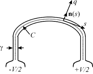
Figure 1: Elliptically shaped quantum wire.

II Schrödinger Equation

In this section we will follow the approach proposed in Ref. daCosta . Let us consider an electron with effective mass $m$ moving in a quantum wire along a curve $C$ which is constructed by a prior confinement potential $V_{\gamma}$. For the sake of simplicity, we start from two-dimensional motion. We introduce the orthonormal coordinate system foot3 $(s,q)$, where $s$ is the arc length parameter and $q$ is the coordinate along the normal $\overrightarrow{n}=\overrightarrow{n}(s)$ to the reference curve $C$. Then the curve $C$ is described by a vector valued function $\overrightarrow{r}(s)$ of the arc length $s$. So, the position in proximity to the curve $C$ is described by

$$\overrightarrow{R}(s,q)=\overrightarrow{r}(s)+q\cdot\overrightarrow{n}(s).$$ (2)

To obtain a meaningful result the particle wave function should be ”uniformly compressed” into a curve, avoiding in this way the tangential forces daCosta , Switkes , Magarill . So, we consider $V_{\gamma}$ to be dependent only on the $q$ coordinate which describes the displacement from the reference curve $C$, this means that points with the same $q$ coordinate but different $s$ coordinates (which describe the position on curve $C$) have the same potential. This potential contains small parameter $\gamma$ so that the potential increases sharply for every small displacement in the normal direction; $\gamma$ is a characteristic width of the potential well $V_{\gamma}$ (the simplest examples of such a potential are the rectangular well potential and the parabolic-trough potential, albeit the real potential would likely be the combination of both). So, the small parameter of the problem is $\gamma/R\ll 1$ Exner .

The motion of the electron obeys the time-independent Schrödinger equation which has the form

$$-\frac{\hbar^{2}}{2m}\triangle_{s,q}\psi+V_{\gamma}(q)\psi=\varepsilon\psi,$$ (3)

where the Laplacian is

$$\triangle_{s,q}=\frac{1}{h}\frac{\partial}{\partial s}\frac{1}{h}\frac{\partial}{\partial s}+\frac{1}{h}\frac{\partial}{\partial q}h\frac{\partial}{\partial q},$$ (4)

with $h$ being the Lamé coefficient (corresponding to the longitudinal coordinate $s$) which depends thanks to Frenet equation upon the curvature $k=k(s)$:

$$h=1-k(s)\cdot q.$$ (5)

In order to eliminate the first-order derivative with respect to $q$ from Eq.(3) we naturally introduce foot4 new wave function $\widetilde{\psi}:$

$$\widetilde{\psi}(s,q)=\sqrt{h}\psi(s,q),$$ (6)

which is, as a matter of fact, the wave function introduced in Ref. daCosta which is normalized so that

$$\int dsdq\left|\widetilde{\psi}(s,q)\right|^{2}=1.$$ (7)

And then the Schrödinger equation Eq.(3) yields

$$-\frac{\hbar^{2}}{2m}\left(\frac{\partial}{\partial s}\frac{1}{h^{2}}\frac{\partial}{\partial s}+\frac{\partial^{2}}{\partial q^{2}}\right)\widetilde{\psi}+V_{eff}(s,q)\widetilde{\psi}+V_{\gamma}(q)\widetilde{\psi}=\varepsilon\widetilde{\psi},$$ (8)

where

$$V_{eff}(s,q)=-\frac{\hbar^{2}}{2m}\left(h^{-2}\frac{k^{2}}{4}+\frac{q}{2}h^{-2}\frac{d^{2}k}{ds^{2}}+\frac{5q^{2}}{4}h^{-4}\left(\frac{dk}{ds}\right)^{2}\right),$$ (9)

which is in agreement with Refs. Exner , Clark2 .

One should be careful with Eq.(8) in order to avoid mistakes found in literature Clark , Magarill . First, we can not decompose this equation, which contains terms which are functions of both $s$ and $q,$ into two equations introducing $\widetilde{\psi}(s,q)=\chi_{n}(q)\chi_{t}(s)$ as in Ref. Clark , where authors have obtained the Eq.(31) for $\chi_{t}(s)$ with coefficients depending on the $q$ variable. To understand another mistake Magarill , consider Eq.(8) within the perturbation theory on small parameter $\gamma$ [comparatively with $R$] (see also in Ref. Exner2 ). Expand $h^{-2}\$and $V_{eff}$ in series in $q\lesssim\gamma,$ writing down explicitly the zeroth term:

$$h^{-2}=1+\sum_{l=1}^{\infty}f_{l}(s)q^{l},$$

$$V_{eff}(s,q)=-\frac{\hbar^{2}}{2m}\left(\frac{k^{2}(s)}{4}+\sum_{l=1}^{\infty}y_{l}(s)q^{l}\right).$$

Then Eq.(8) can be rewritten:

$$\left(\widehat{H}_{0}+\widehat{V}\right)\widetilde{\psi}=\varepsilon\widetilde{\psi},$$ (10)

where

$$\widehat{H}_{0}=-\frac{\hbar^{2}}{2m}\left(\frac{\partial^{2}}{\partial s^{2}}+\frac{\partial^{2}}{\partial q^{2}}\right)-\frac{\hbar^{2}}{2m}\frac{k^{2}(s)}{4}+V_{\gamma}(q),$$ (11)

$$\widehat{V}=\frac{\hbar^{2}}{2m}\sum_{l=1}^{\infty}q^{l}\left(-\frac{\partial}{\partial s}f_{l}(s)\frac{\partial}{\partial s}+y_{l}(s)\right),$$ (12)

we notice that $\widehat{V}$ is a second order in the variable $s$ differential operator. The solution of Eq. (10) is

$$\widetilde{\psi}=\widetilde{\psi}^{(0)}+\sum_{l=1}^{\infty}\widetilde{\psi}^{(l)},$$

where $\widetilde{\psi}^{(l)}\sim\gamma^{l}$ and $\widetilde{\psi}^{(0)}$ corresponds to the zeroth-order approximation problem: $\widehat{H}_{0}\widetilde{\psi}^{(0)}=\varepsilon\widetilde{\psi}^{(0)}$. This equation can be decomposed by separating the wave function: $\widetilde{\psi}(s,q)=\eta(q)\chi(s)$:

$$-\frac{\hbar^{2}}{2m}\frac{d^{2}}{dq^{2}}\eta+V_{\gamma}(q)\eta=E_{t}\eta$$ (13)

and

$$-\frac{\hbar^{2}}{2m}\frac{d^{2}}{ds^{2}}\chi+V_{eff}(s)\chi=E_{l}\chi,$$ (14)

where $V_{eff}(s)$ is given by Eq.(1); $\varepsilon=E_{t}+E_{l}$; $R=k(s)^{-1}$ is the curvature radius (in the next section we omit the subscript ”$l$”, identifying energy $E$ with its longitudinal component $E_{l}$). Eq.(13) describes the confinement of the electron to a $\gamma$-neighborhood of the curve $C$ and Eq.(14) describes the motion along the $s$ coordinate (along the curve $C$). In fact, Eq.(14) is a conventional one-dimensional Schrödinger equation for an electron moving in the $s$-dependent potential $V_{eff}(s)$; the latter connects the geometry and the dynamical equation. The origin of this potential is in the wavelike properties of the particles; $V_{eff}$ is essential for not large $R/\lambda_{F}.$ We underline that the effective potential (Eq.(1)) in the zeroth-order approximation in $\gamma/R$ is not dependent on the method of  ”one-dimensionalization”, i.e. on the choice of $V_{\gamma}(q)$ (compare this conclusion with the one derived in Ref. Magarill ).

We also note that if we have started from the three-dimensional equation of motion we would obtain an additional effective potential which in the planar situation is zero daCosta .

III Conductance

The conductance $G$ of quantum contacts can be related to the transmission probability $T(E)$ by Landauer’s formula Landauer . At zero temperature and finite voltages $V$ it takes the form

$$G=\frac{G_{0}}{2}[T(E_{F}+\frac{eV}{2})+T(E_{F}-\frac{eV}{2})]$$ (15)

where $G_{o}=2e^{2}/h,$ $E_{F}$ is the Fermi energy. Two terms in this equation correspond to two electronic beams moving in opposite directions and differing in bias energy. So, we are interested in the transmission probability $T(E)$ with $E$ being an electron energy.

In this section we consider the curve $C$ to consist of three ideally connected parts (see Fig.1): (i) linear ($s<0$), (ii) elliptical ($0<s<l$, $l$ is half of the ellipse’s perimeter), and (iii) one more linear domain ($s>l$). We consider wave functions in the regions (i) and (iii) to be plane waves $\psi_{1}=e^{ik_{1}s}+re^{-ik_{1}s},$ $\psi_{3}=te^{ik_{1}s}$, where $k_{1}=\sqrt{2mE/\hbar^{2}}$ is the wave vector and $t$ and $r$ are the transmission and reflection coefficients; the transmission probability is given by $T=\left|t\right|^{2}$. The wave function $\psi_{2}\equiv\chi$, where $\chi$ is the solution of Eq.(14), with the effective potential given by Eq.(1). The  curvature can be written most simply in the elliptical $v$ coordinate Whittaker which is defined with its Lamé coefficient

$$H=ds/dv=a\sqrt{1-e^{2}\cos^{2}v},$$ (16)

where $e$ is the eccentricity of an ellipse and $a$ is the length of its major semiaxis; we apply $v(s=0)=0$. Then the effective (geometrical) potential (see Eq.(1)) can be written as

$$V_{eff}(s)=-\frac{\hbar^{2}}{8ma^{2}}\frac{1-e^{2}}{(1-e^{2}\cos^{2}v)^{3}},$$ (17)

which is in agreement with Ref.Switkes .

We introduce new wave function

$$\xi(v(s))=\chi(s)/\sqrt{H},$$ (18)

for which the equation takes the form (see Eqs. (14), (16)-(18)):

$$\frac{d^{2}}{dv^{2}}\xi+\left[\frac{2ma^{2}}{\hbar^{2}}E\cdot g(v)+U(v)\right]\xi=0,$$ (19)

$$U(v)=\frac{5}{4}\frac{1-e^{2}}{g^{2}}-\frac{1-e^{2}/2}{g}-\frac{e^{4}}{16}\frac{\sin^{2}2v}{g^{2}},$$ (20)

where $g=H^{2}/a^{2}=1-e^{2}\cos^{2}v.$ Eq.(19) is the Hill’s equation with $\pi$-periodic coefficients; fundamental system of its solutions is Kamke

$$\xi_{\pm}=e^{\pm i\mu v}y(\pm v),$$ (21)

where $y(v)$ is a $\pi$-periodic function, $\mu$ is the characteristic exponent. Then (see Eqs.(18) and (21)):

$$\chi=C_{1}e^{i\mu v}\widetilde{y}(v)+C_{2}e^{-i\mu v}\widetilde{y}(-v),$$ (22)

(here $\widetilde{y}(v)\equiv\sqrt{H}y(v)$).

Thus, we know what wave functions are like and now we are interested in $T=\left|t\right|^{2}$ which describes transmission over potential well (see Eq.(17)). Then we make use of the conditions of continuity of the wave function and of its derivative, so we obtain the system of four equations which is similar to one given in Ref. LL ; and so is the result:

$$T=\left[1+\frac{1}{4}\left(\kappa-\frac{1}{\kappa}\right)^{2}\sin^{2}\pi\mu\right]^{-1}$$ (23)

where we denoted

$$\kappa=-\frac{i}{ak_{1}\sqrt{1-e^{2}}}\left(\frac{\xi_{+}^{\prime}}{\xi_{+}}\right)_{v=0}.$$ (24)

(To get Eq.(23) we applied that $\mu$ and $\kappa$ are real, which is straightforward to proof.)

IV Results and discussion

To understand how the conductivity $G$ depends on the bias $eV$ and the geometry we need to find the solution of Hill’s equation Eq.(19). We did this numerically as well as within the perturbation theory for an ellipse which is close to a circle (i.e. $e^{2}\ll 1$); we found that both are in good agreement for $e<1/2$. In the zeroth-order approximation in $e^{2}$ (i.e. for $e=0$, the case of a circular arc) we have $\mu_{0}=ak_{2}$ and $\kappa_{0}=k_{2}/k_{1},$ where $k_{2}=\sqrt{2mE/\hbar^{2}+1/4a^{2}}$ (see also in Ref. Yu.A. ). This means that one can observe oscillations in $G(V)$ dependence provided $a\gtrsim\lambda_{F}$ and the amplitude of these oscillations is enough small.

The first-order approximation of the perturbation theory (for $a>\lambda_{F}$) yields:

$$\mu\simeq\mu_{0}+e^{2}\mu_{1},\kappa\simeq\kappa_{0}+e^{2}\kappa_{1};$$ (25)

with

$$\mu_{1}=-ak_{1}^{2}/4k_{2}\equiv-\mu_{0}/4\kappa_{0},$$ (26)

$$\kappa_{1}=k_{1}/[4k_{2}((ak_{2})^{2}-1)].$$ (27)

Then we solve Hill’s equation Eq.(19) numerically. The characteristic exponent $\mu$ is defined via the solution of Eq.(19) with the initial conditions: $\xi_{1}(0)=1,$ $\xi_{1}^{\prime}(0)=0$, and then $\mu$ is the solution of the equation$\ \xi_{1}(\pi)=\cos\pi\mu$ (see in Ref. Kamke ). More challenging is to find $\xi_{+}$ (see Eq.(21)), which can be formulated as the boundary value problem with Eq.(19) and boundary conditions $\xi_{2}(0)=0,$ $\xi_{2}(\pi)=\sin\pi\mu$ (where $\xi_{2}(v)=\mathop{\mathrm{I}m}\xi_{+}(v))$. We introduce $\xi_{3}(v)=\xi_{2}(v)/\xi_{2}^{\prime}(0)$, and so we have initial conditions problem for $\xi_{3}(v)$ ($\xi_{3}(0)=0,$ $\xi_{3}^{\prime}(0)=1$), the solution of which gives what we seek for to define $\kappa$: $\left(\xi_{+}^{\prime}/\xi_{+}\right)_{v=0}=\xi_{2}^{\prime}(0)=\sin\pi\mu/\xi_{3}(\pi)$. The results of the described procedure are numerically plotted at Figs.2 and 3 which is for enough elongated ellipse with $e=0.99$ (so that $a/b=7,$ where $a$ and $b$ are the lengths of its major and minor semiaxes respectively). We note about Fig. 3 that, being restricted by the condition $R\gg\gamma$, we should not tend $a$ to $0$, namely, we may suppose $R\gg\gamma$ for $a/\lambda_{F}\sim 10$ but may not for $a/\lambda_{F}\lesssim 1$ [for $e$ close to $1$]. We also note that Eq.(15) is, strictly speaking, correct for $eV$ small compared with $E_{F}$ and describes $G(V)$  dependence for $eV\sim E_{F}$ qualitatively. We conclude that $e$ close to $1$ increases significantly oscillations in comparison with $e=0$ case; the amplitude of oscillations in $G=G(V)$ dependence is defined by the value of $a/\lambda_{F}$.

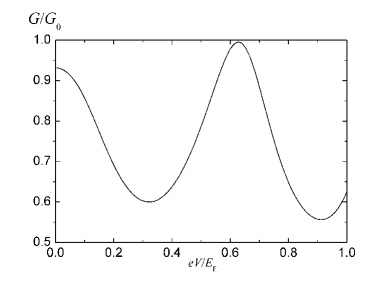
Figure 2: Conductance as a function of the bias $G=G(eV)$ at $e=0.99$, $a=10\lambda_{F}$ (at the same value of $a$ but $e=0$ the amplitude $\Delta G/G_{0}$ is of order of $10^{-5}$).

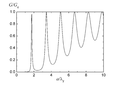
Figure 3: Conductance as a function of the length of the major semiaxis $G=G(a)$ at $e=0.99$, $V=0$.

In summary, we have rederived the quantum-mechanical effective potential induced by curvature of one-dimensional quantum wire. We have shown that for any confining potential $V_{\gamma}$, depending only on the displacement $q$ from the reference curve $C$, this effective potential is universal: it does not depend on the choice of $V_{\gamma}$ and is given by Eq.(1). And then we have studied the effect of the curvature in the zeroth-order approximation in the width of the wire on the conductance of an ideal elliptically shaped quantum wire. It has been shown, in particular, that, due to the effect of the curvature, dependence of the conductance $G(V)$ on the applied bias changes drastically. So, the effect of the curvature can be observed by measuring the conductance of a quantum wire. On the other hand, one can change the characteristics of the quantum wire, such as conductance, setting its size, shape, or applied bias.

One of the authors (S.N.S.) would like to thank Prof. I.D. Vagner for his warm hospitality during the stay at Grenoble High Magnetic Field Laboratory (France) where the part of this work was done. We also thank Prof. A.M. Kosevich for critical discussion of the manuscript.

References

- (1) We study here only one-channel wire when only the lowest subband is occupied.
- (2) H. Jensen and H. Koppe, Ann. of Phys.63, 586 (1971).
- (3) R.C.T. da Costa, Phys. Rev. A23,1982 (1981).
- (4) J. Marcus, J. Chem. Phys. 45, 4493 (1966).
- (5) E.Switkes, E.L. Russell, and J.L. Skinner, J. Chem. Phys. 67, 3061 (1977).
- (6) P. Exner and P. Šeba, J. Math. Phys. 30, 2574 (1989).
- (7) P. Duclos and P. Exner, Rev. Math. Phys. 7, 73 (1995).
- (8) I.J. Clark and A.J. Bracken, J. Phys. A29, 339 (1996).
- (9) I.J. Clark and A.J. Bracken, J. Phys. A29, 4527 (1996).
- (10) L.I. Magarill, D.A. Romanov, and A.V. Chaplik, JETP 83, 361 (1996).
- (11) L.I. Magarill and A.V. Chaplik, JETP Lett. 68, 148 (1998).
- (12) L.I. Magarill, D.A. Romanov, and A.V. Chaplik, Usp. Fiz. Nauk 170, 325 (2000).
- (13) A. Namiranian, M.R.H. Khajehpour, Yu.A. Kolesnichenko, and S.N. Shevchenko, to be published in Physica E (2001).
- (14) V.Ya. Prinz, V.A. Seleznev, V.A. Samoylov, and A.K. Gutakovsky, Microelectron. Eng. 30, 439 (1996).
- (15) M. Kugler and S. Shtrikman, Phys. Rev. D37, 934 (1988).
- (16) R.Y. Chiao and Y.S. Wu, Phys. Rev. Lett. 57, 933 (1986); A. Tomita and R.Y. Chiao, ibid. 57, 937 (1986).
- (17) J. Goldstone and R.L. Jaffe, Phys. Rev. B45, 14100 (1992).
- (18) We consider here only flat curves and we refer the reader who is interested in the effect of the torsion to Ref. Clark .
- (19) The advantages of establishing from the very beginning the coordinate system are that it allows the most general consideration and that [because of the diagonal structure of the metric tensor] we can in the zeroth-order approximation in the width of the quantum wire decompose the dynamical equation of motion into two.
- (20) We do this to eliminate terms of the form which in Ref. Jensen were called ”dangerous terms”. We cannot apply since : although but and, so, the second term in the brackets is and that is the order of terms we are interested in below.
- (21) R.Landauer, IBM J. Res. Dev. 1, 233 (1957).
- (22) E.T. Whittaker and G.N. Watson, A Course of Modern Analysis, Cambridge University Press; Cambridge (1927).
- (23) E. Kamke, Gewöhnliche Differentialgleichungen, Leipzig (1959) [Russ. transl., Nauka, Moskow, 1965].
- (24) L.D. Landau and E.M. Lifshits, Quantum Mechanics: Non-relativistic Theory, Pergamon Press, Oxford (1965).