Inverted Berezinskii-Kosterlitz-Thouless Singularity and High-Temperature Algebraic Order in an Ising Model on a Scale-Free Hierarchical-Lattice Small-World Network

Abstract

We have obtained exact results for the Ising model on a hierarchical lattice incorporating three key features characterizing many real-world networks—a scale-free degree distribution, a high clustering coefficient, and the small-world effect. By varying the probability $p$ of long-range bonds, the entire spectrum from an unclustered, non-small-world network to a highly-clustered, small-world system is studied. Using the self-similar structure of the network, we obtain analytic expressions for the degree distribution $P(k)$ and clustering coefficient $C$ for all $p$, as well as the average path length $\ell$ for $p=0$ and $1$. The ferromagnetic Ising model on this network is studied through an exact renormalization-group transformation of the quenched bond probability distribution, using up to 562,500 renormalized probability bins to represent the distribution. For $p<0.494$, we find power-law critical behavior of the magnetization and susceptibility, with critical exponents continuously varying with $p$, and exponential decay of correlations away from $T_{c}$. For $p\geq 0.494$, in fact where the network exhibits small-world character, the critical behavior radically changes: We find a highly unusual phase transition, namely an inverted Berezinskii-Kosterlitz-Thouless singularity, between a low-temperature phase with non-zero magnetization and finite correlation length and a high-temperature phase with zero magnetization and infinite correlation length, with power-law decay of correlations throughout the phase. Approaching $T_{c}$ from below, the magnetization and the susceptibility respectively exhibit the singularities of $\exp(-C/\sqrt{T_{c}-T})$ and $\exp(D/\sqrt{T_{c}-T})$, with $C$ and $D$ positive constants. With long-range bond strengths decaying with distance, we see a phase transition with power-law critical singularities for all $p$, and evaluate an unusually narrow critical region and important corrections to power-law behavior that depend on the exponent characterizing the decay of long-range interactions.

PACS numbers: 89.75.Hc, 64.60.Ak, 75.10.Nr, 05.45.Df

I Introduction

Complex networks provide an intriguing avenue for tackling one of the long-standing questions in statistical physics: how the collective behavior of interacting objects is influenced by the topology of those interactions. Inspired by the diversity of network structures found in nature, researchers in recent years have investigated a variety of statistical models on networks with real-world characteristics AlbertBarabasi ; Newman ; DoroRev . Three empirically common network types have been the focus of attention: networks with large clustering coefficients, where all neighbors of a node are likely to be neighbors of each other; networks with “small-world” behavior in the average shortest-path length, $\ell\sim\ln(N)$, where $N$ is the number of nodes; and those with a power-law (scale-free) distribution of degrees. Since the pioneering network models of Watts-Strogatz WattsStrogatz , which exemplified the first two properties, and Barabási-Albert BarabasiAlbert , which showed how the third could arise from particular mechanisms of network growth, significant advances have taken place in understanding how these properties affect statistical systems. The Ising model has been studied on small-world networks Gitterman ; BarratWeigt ; Pekalski ; Hong ; Jeong , along with the $XY$ model Kim , and on Barabási-Albert scale-free networks Aleksiejuk ; Bianconi . On random graphs with arbitrary degree distributions, the Ising model shows a range of possible critical behaviors depending on the moments of the distribution (or in the specific case of scale-free distributions, the exponent describing the power-law tail) Doro1 ; Leone , a fact which is accounted for by a phenomenological theory of critical phenomena on these types of networks Goltsev .

In the current work we introduce a novel network structure based on a hierarchical lattice BerkerOstlund ; Kaufman ; Kaufman2 augmented by long-range bonds. By changing the probability $p$ of the long-range bonds, we observe an entire spectrum of network properties, from an unclustered network for $p=0$ with $\ell\sim N^{1/2}$, to a highly-clustered small-world network for $p=1$ with $\ell\sim\ln N$. In addition, the network has a scale-free degree distribution for all $p$. Due to the hierarchical construction of the network, together with the stochastic element introduced through the attachment of the long-range bonds, this network combines features of deterministic and random scale-free growing networks Barabasi2 ; Doro4 ; Doro3 ; ComellasSampels ; Jung ; ZhangRong ; Andrade ; Zhou ; AndradeHerrmann , and in the $p=1$ limit its geometrical properties are similar to the pseudofractal graph studied in Ref. Doro3 . The self-similar structure of the network allows us to calculate analytic expressions for the degree distribution and clustering coefficient for all $p$, as well as the average shortest-path length $\ell$ in the limiting cases $p=0$ and $1$.

A renormalization-group transformation is formulated for the Ising model on the network, yielding a variety critical behaviors of thermodynamic densities and response functions. For the quenched disordered system at intermediate $p$, we study the Ising model through an exact renormalization-group transformation of the quenched bond probability distribution, implemented numerically using up to 562,500 renormalized probability bins to represent the distribution. We find a finite critical temperature at all $p$, with two distinct regimes for the critical behavior. When $p<0.494$, the magnetization and susceptibility show power-law scaling, and away from $T_{c}$ correlations decay exponentially, as in a typical second-order phase transition. The magnitudes of the critical exponents, which continuously vary with $p$, become infinite as $p\to 0.494$ from below. For $p\geq 0.494$, in fact coinciding with the onset of the small-world behavior of the underlying network, we find a highly unusual infinite-order phase transition: an inverted Berezinskii-Kosterlitz-Thouless singularity Berezinskii ; KosterlitzThouless , between a low-temperature phase with non-zero magnetization and finite correlation length, and a high-temperature phase with zero magnetization and infinite correlation length, exhibiting power-law decay of correlations (in contrast to the typical Berezinskii-Kosterlitz-Thouless phase transition, where the algebraic order is in the low-temperature phase). Approaching $T_{c}$ from below, the magnetization and the susceptibility respectively behave as $\exp(-C/\sqrt{T_{c}-T})$ and $\exp(D/\sqrt{T_{c}-T})$, with $C$ and $D$ calculated positive constants.

Infinite-order phase transitions have been observed for the Ising model on random graphs with degree distributions $P(k)$ that have a diverging second moment $\langle k^{2}\rangle$ Doro1 ; Leone , but for these systems $T_{c}=\infty$ on an infinite network. An infinite-order percolation transition has been seen in models of growing networks Callaway ; Doro5 ; Kim2 ; Lancaster ; Bauer2 ; Coulomb ; Bollobas ; Krapivsky , with exponential scaling in the size of the giant component above the percolation threshold. A prior observation of a finite-temperature, inverted Berezinskii-Kosterlitz-Thouless singularity similar to the one described above was made in Ising models on an inhomogeneous growing network Bauer and on a one-dimensional inhomogeneous lattice Costin1 ; Costin2 ; Bundaru ; Romano .

The final aspect of our network we investigated was the effect of adding distance-dependence to the interaction strengths of the long-range bonds, along the lines of Ref. Jeong , where distance-dependent interactions were considered in a small-world Ising system. With decaying interactions, the second-order phase transition for all $p$ has a strongly curtailed critical region and corrections to power-law behavior that vary with the exponent $\sigma$ describing the decay of interactions.

This paper is organized as follows: In Sec. II, we describe the basic geometric features of the network, starting with the construction of the lattice (II.A), whose deterministic nature allows us to derive exact results on the degree distribution (II.B.1), clustering coefficient (II.B.2), and average shortest-path length (II.B.3). Additional details about the derivations in this section are included in Appendix A. In Sec. III, we study the Ising model on the network through exact renormalization-group transformations, first for the simpler cases where the long-distance bonds are either all absent (III.A), or all present (III.B). In the latter case, we look at both uniform interaction strengths along the long-distance bonds (III.B.1) and interactions decaying with distance (III.B.2). Finally, we turn to the more complex situation where there is a quenched random distribution of the long-distance bonds in the lattice, which requires formulating a renormalization-group transformation in terms of quenched probability distributions (III.C.1). Analysis of the flows of these distributions gives a complete picture of the thermodynamics of our system over the entire range of $p$ (III.C.2). We present our conclusions in Sec. IV.

II Hierarchical-Lattice Small-World Network

II.1 Construction of the Lattice

We construct a hierarchical lattice BerkerOstlund ; Kaufman ; Kaufman2 as shown in Fig. 1. The lattice has two types of bonds: nearest-neighbor bonds (depicted as solid lines) and long-range bonds (depicted as dashed lines). In each step of the construction, every nearest-neighbor bond is replaced either by the connected cluster of bonds on the top right of Fig. 1 with probability $p$, or by the connected cluster on the bottom right with probability $1-p$. This procedure is repeated $n$ times, with the infinite lattice obtained in the limit $n\to\infty$. The initial ($n=0$) lattice is two sites connected by a single nearest-neighbor bond. An example of the lattice at $n=4$ for an arbitrary $p\neq 0,1$ is shown in Fig. 2.

The $p=0$ case, with no long-range bond, is the hierarchical lattice  BerkerOstlund on which the Migdal-Kadanoff Migdal ; Kadanoff recursion relations with dimension $d=2$ and length rescaling factor $b=2$ are exact. As will be seen below, the network in this case exhibits no small-world feature, with a clustering coefficient $C=0$ and an average shortest-path length $\ell$ that scales like $N^{1/2}$, where $N$ is the number of sites in the lattice. The $p=1$ case, on the other hand, shows typical small-world properties, with the presence of long-range bonds giving the high clustering coefficient $C=0.820$ and an average path length which scales more slowly with system size, $\ell\sim\ln N$. By varying the parameter $p$ from 0 to 1, we continuously move between the two limits. These and other network characteristics of our hierarchical lattice are discussed in detail in the next section.

Figure 1: Construction of the hierarchical lattice. The solid lines correspond to nearest-neighbor bonds, while the dashed lines are long-range bonds, which occur with probability p.

Figure 2: An example of the hierarchical lattice after $n=4$ steps in the construction, for $p=0.6$.

II.2 Network Characteristics

II.2.1 Degree Distribution

After the $n$th step of the construction, there are a total of $N_{n}=\frac{2}{3}(2+4^{n})$ sites in the lattice. We categorize these sites by the number of nearest-neighbor bonds attached to the site, $k_{\text{nn}}$, and the maximum possible number of long-range bonds attached to the site, $k_{\text{ld}}$, of which on average only $pk_{\text{ld}}$ actually exist. At the $m$th level there are $4^{n-m+1/2}$ sites with $k_{\text{nn}}=2^{m}$, $k_{\text{ld}}=2^{m}-2$, for $m=1,\ldots,n$. In addition, there are two sites with $k_{\text{nn}}=2^{n}$, $k_{\text{ld}}=2^{n}-1$. Thus, the non-zero probabilities that a randomly chosen site has degree $k$ are

$$P_{n}(k)=\begin{cases}\frac{4^{n-m+1/2}}{N_{n}}\binom{2^{m}-2}{r}p^{r}(1-p)^{2^{m}-2-r},\\ \frac{2}{N_{n}}\binom{2^{n}-2}{r}p^{r}(1-p)^{2^{n}-2-r}\\ \qquad+\frac{2}{N_{n}}\binom{2^{n}-1}{r}p^{r}(1-p)^{2^{n}-1-r},\\ \frac{2}{N_{n}}p^{2^{n}-1},\end{cases}$$ (1)

respectively for

$$k= 2^{m}+r,\>0\leq r\leq 2^{m}-2,\>1\leq m\leq n-1,$$

$$k= 2^{n}+r,\>0\leq r\leq 2^{n}-2,$$

$$k= 2^{n+1}-1.$$ (2)

Since the degree distribution is not continuous, the exponent describing the power-law decay of degrees is extracted from the cumulative distribution function Newman in the $n\to\infty$ limit, $P_{\text{cum}}(k)=\sum_{k^{\prime}=k}^{\infty}P(k^{\prime})$, where $P(k)=\lim_{n\to\infty}P_{n}(k)$. For a scale-free network of exponent $\alpha$, $P_{\text{cum}}(k)\sim k^{1-\alpha}$. In our case $P_{\text{cum}}(k)\sim k^{-2}$ for large $k$, giving $\alpha=3$, a value comparable to the exponents of many real-world scale-free networks AlbertBarabasi . The maximum degree $k_{\text{max}}$ in the scale-free network should scale as $k_{\text{max}}\sim N^{1/(\alpha-1)}_{n}$ Newman , which is indeed satisfied, for large $n$, in our network. The average degree $\langle k\rangle_{n}$ after $n$ construction steps is

$$\langle k\rangle_{n}=\sum_{k=1}^{\infty}kP_{n}(k)=3+p-\frac{3(2+p)}{2+4^{n}}\,,$$ (3)

which goes to $\langle k\rangle=3+p$ in the infinite lattice limit.

II.2.2 Clustering Coefficient $C_{m}$

If a given site in the network is connected to $k$ sites, defined as the neighbors of the given site, the ratio between the number of bonds among the neighbors and the maximum possible number of such bonds $k(k-1)/2$ is the clustering coefficient of the given site WattsStrogatz . The clustering coefficient $C$ of the network is the average of this coefficient over all the sites, and can take on values between 0 and 1, the latter corresponding to a maximally clustered network where all neighbors of a site are also neighbors of each other. For our network in the $n\to\infty$ limit, $C$ can be evaluated exactly: The fraction $\lim_{n\to\infty}4^{n-m+1/2}/N_{n}=3\cdot 4^{-m}$ of the sites, with $k_{\text{nn}}=2^{m}$ and $k_{\text{ld}}=2^{m}-2$, have the average clustering coefficient $C_{m}$, where $C_{1}=p$ and $C_{m}$ for $m>1$ is, as derived in Appendix A.1,

$$C_{m}=\sum_{r=0}^{2^{m-1}}\sum_{r^{\prime}=0}^{2^{m-1}-2}\binom{2^{m-1}}{r}\binom{2^{m-1}-2}{r^{\prime}}\cdot\\ \frac{2p^{r+r^{\prime}}(1-p)^{2^{m}-2-r-r^{\prime}}\left\{2r+p\binom{r+r^{\prime}}{2}\frac{2^{m}-3}{\binom{2^{m}-2}{2}}\right\}}{(2^{m}+r+r^{\prime})(2^{m}+r+r^{\prime}-1)}\,.$$ (4)

We plot the clustering coefficient $C$

$$C=\sum_{m=1}^{\infty}3\cdot 4^{-m}C_{m}\,.$$ (5)

as a function of $p$ in Fig. 3. Note that $C$ increases almost linearly from $0$ at $p=0$ to $0.820$ at $p=1$, as can also be seen from the expansion of Eq. (5) to second order in $p$,

$$C=0.837p-0.0378p^{2}+\text{O}(p^{3})\,.$$ (6)

Figure 3: Clustering coefficient $C$ for the infinite lattice as a function of the probability of long-range bonds $p$.

II.2.3 Average Shortest-Path Length $\ell_{n}$

Let $d_{ij}$ be the shortest-path length between two sites $i$ and $j$ in the network, measured in terms of the number of bonds along the path. The average shortest-path length $\ell_{n}$ is the average of $d_{ij}$ over all pairs of sites $i$,$j$ at the $n$th level. For general $p$ we have evaluated this quantity numerically. For $p=0$ and $p=1$ we have obtained exact analytic expressions (Appendix A.2), revealing qualitatively distinct behaviors: For $p=0$ we find

$$\ell_{n} =\frac{2^{n}(98+27\cdot 2^{n}+42\cdot 4^{n}+22\cdot 16^{n}+21n\cdot 4^{n})}{21(2+5\cdot 4^{n}+2\cdot 16^{n})}$$

$$\xrightarrow[n\to\infty]{}\frac{11}{21}2^{n}\,,$$ (7)

and since $N_{n}\sim 4^{n}$ for large $n$, we have $\ell_{n}\sim N_{n}^{1/2}$. Comparing this result to that of a hypercubic lattice of dimension $d$, where the average shortest-path length scales as $N^{1/d}$ AlbertBarabasi , we see that $\ell_{n}$ for the $p=0$ network has the power-law scaling behavior of the square lattice. For $p=1$, on the other hand, we find

$$\ell_{n}=$$

$$\frac{23+4\cdot(-2)^{n}+44\cdot 4^{n}+10\cdot 16^{n}+6n\cdot 4^{n}+12n\cdot 16^{n}}{9(2+5\cdot 4^{n}+2\cdot 16^{n})}$$

$$\xrightarrow[n\to\infty]{}2n/3~{},$$ (8)

which means that $\ell_{n}\sim\ln(N_{n})$ for large $n$. This much slower, logarithmic scaling of $\ell_{n}$ with lattice size, together with the high clustering coefficient, are the defining features of a small-world network.

In Fig. 4 we show $\ell_{n}$ calculated for for the full range of $p$ between 0 and 1, for $n$ up to 6. It is evident that even a small percentage of long-range bonds drastically reduces the average shortest-path length, and that $\ell_{n}$ shows small-world characteristics, scaling nearly linearly with $n$, for $p\gtrsim 0.5$. We shall see below that the small-world structure at larger $p$ translates into a distinctive critical behavior for the Ising model on this network.

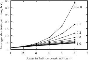
Figure 4: Average shortest-path length $\ell_{n}$ for level $n$, shown for various values of $p$ between 0 and 1. For $p=0$ and $p=1$, $\ell_{n}$ is given exactly by Eqs. (II.2.3) and (II.2.3). For other $p$, we have calculated $\ell_{n}$ numerically, with an accuracy of $\pm 0.3\%$.

III Ising Model on the Network

We study the Ising model on the network introduced in the previous section, with Hamiltonian

$$-\beta{\cal H}= J\sum_{\langle ij\rangle_{\text{nn}}}s_{i}s_{j}+\sum_{\langle ij\rangle_{\text{ld}}}K_{ij}s_{i}s_{j}$$

$$+H_{B}\sum_{\langle ij\rangle_{\text{nn}}}(s_{i}+s_{j})+H_{S}\sum_{i}s_{i}\,,$$ (9)

where $J,K_{ij}>0$, $\langle ij\rangle_{\text{nn}}$ denotes summation over nearest-neighbor bonds, and $\langle ij\rangle_{\text{ld}}$ denotes summation over long-range bonds. We generalize the above, by introducing a distance dependence in the interaction constants $K_{ij}$,

$$K_{ij}=Jm_{ij}^{-\sigma}\,.$$ (10)

Here the exponent $\sigma\geq 0$, and $m_{ij}$ measures the range of the long-range bond between sites $i$ and $j$: For a lattice constructed in $n$ steps, those long-range bonds that appear at the $n$th step have $m_{ij}=1$, those that appear at the $(n-1)$th step have $m_{ij}=2$, and so on until the long-range bond that appears at the first step, which has $m_{ij}=n$. The long-range term in the Hamiltonian can be rewritten as

$$\sum_{\langle ij\rangle_{\text{ld}}}K_{ij}s_{i}s_{j}=K_{1}\sum_{\langle ij\rangle_{\text{ld},1}}s_{i}s_{j}+K_{2}\sum_{\langle ij\rangle_{\text{ld},2}}s_{i}s_{j}+\cdots\,,$$ (11)

where $K_{q}\equiv Jq^{-\sigma}$ and $\langle ij\rangle_{\text{ld},q}$ denotes summation over long-range bonds with $m_{ij}=q$.

The Hamiltonian of Eq. (9) includes two types of magnetic field terms, one counted with bonds ($H_{B}$) and the other counted with sites ($H_{S}$). We shall calculate the associated spontaneous magnetizations at $H_{B}=H_{S}=0$,

$$M_{B}=\frac{1}{N_{\text{nn}}}\sum_{\langle ij\rangle_{\text{nn}}}\langle s_{i}+s_{j}\rangle\,,\quad M_{S}=\frac{1}{N_{\text{n}}}\sum_{i}\langle s_{i}\rangle\,,$$ (12)

where $N_{\text{nn}}=4^{n}$ is the number of nearest-neighbor bonds after the $n$th construction stage, so that $N_{\text{nn}}/N_{\text{n}}=3/2$ in the limit $n\to\infty$. For a translationally invariant lattice, where each site has the same degree, $M_{B}$ and $M_{S}$ would be simply related by $M_{B}=2M_{S}$, but for the hierarchical lattice this is no longer true due to the different degrees of the sites.

Before turning to the phase diagram and critical properties of the system for general $p$, which require formulating a renormalization-group transformation in terms of quenched probability distributions, we present the distinct critical behaviors of the limiting cases of $p=0$ and $p=1$.

Property		$p=0$	$0<p<0.494$, $\sigma=0$	$0.494\leq p\leq 1$, $\sigma=0$	$0<p<1$, $0<\sigma<1$	$p=1$, $0<\sigma<1$	$0<p\leq 1$, $\sigma\geq 1$
$T_{c}$		1.641	varies with $p$ (see Fig. 12); reaches 3.592 at $p=0.494$	varies with $p$ (see Fig. 12); reaches 7.645 at $p=1$	varies with $\sigma$ and $p$ (see Fig. 8)	varies with $\sigma$ (see Fig. 8); reaches 3.485 at $\sigma=1$	varies with $\sigma$ and $p$ (see Fig. 8)
$y_{T}$		0.747	vary with $p$	0	0.747	0.747	0.747
$y_{H}$		1.879	(see Fig. 14)	1.585	1.879	1.879	1.879
$\xi$		$|t|^{-1/y_{T}}$	$|t|^{-1/y_{T}}$	$e^{A/\sqrt{|t|}}\,(t<0)$	$|t|^{-\frac{1}{y_{T}}+f_{1}(p,\sigma,t)}$	$|t|^{-\frac{1}{y_{T}}-C_{1}\left(-\ln|t|\right)^{-\sigma}}$	$|t|^{-1/y_{T}}$
				$\infty\,(t>0)$
$C_{\text{\scriptsize{ sing}}}$		$|t|^{-\frac{2y_{T}-2}{y_{T}}}$	$|t|^{-{2y_{T}-2}{y_{T}}}$	$|t|^{-3/2}e^{-2A/\sqrt{|t|}}$	$|t|^{-\frac{2y_{T}-2}{y_{T}}+f_{2}(p,\sigma,t)}$	$|t|^{-\frac{2y_{T}-2}{y_{T}}+2C_{1}\left(-\ln|t|\right)^{-\sigma}}$	$|t|^{-\frac{2y_{T}-2}{y_{T}}}$
$M_{B}$, $M_{S}$	$(t<0)$	$|t|^{\frac{2-y_{H}}{y_{T}}}$	$|t|^{\frac{2-y_{H}}{y_{T}}}$	$e^{-A(2-y_{H})/\sqrt{|t|}}$	$|t|^{\frac{2-y_{H}}{y_{T}}+f_{3}(p,\sigma,t)}$	$|t|^{\frac{2-y_{H}}{y_{T}}+C_{2}\left(-\ln|t|\right)^{-\sigma}}$	$|t|^{\frac{2-y_{H}}{y_{T}}}$
$\chi_{BB}$, $\chi_{BS}$, $\chi_{SS}$	$(t<0)$	$|t|^{-\frac{2y_{H}-2}{y_{T}}}$	$|t|^{-\frac{2y_{H}-2}{y_{T}}}$	$e^{A(2y_{H}-2)/\sqrt{|t|}}$	$|t|^{-\frac{2y_{H}-2}{y_{T}}+f_{4}(p,\sigma,t)}$	$|t|^{-\frac{2y_{H}-2}{y_{T}}+C_{3}\left(-\ln|t|\right)^{-\sigma}}$	$|t|^{-\frac{2y_{H}-2}{y_{T}}}$

Table I: Critical properties of the hierarchical-lattice network for all cases of long-range bond probabilities $p$ and long-range bond decay exponents $\sigma$. The functions $f_{i}(p,\sigma,t)$ are corrections to the $p=0$ scaling behavior, which are significant at larger $p$. The factor $A$ is defined below Eq. (37), and $C_{1}$, $C_{2}$, $C_{3}$ are given as functions of $y_{T},y_{H},\sigma$ in Eqs. (62).

III.1 Critical Properties at $p=0$

The $d=2$, $b=2$ Migdal-Kadanoff recursion relations are exact  BerkerOstlund on the $p=0$ lattice, and the renormalization-group transformation consists of decimating the two center sites in the cluster shown on the bottom right of Fig. 1. The renormalized Hamiltonian of the two remaining sites $i^{\prime}$, $j^{\prime}$ is

$$-\beta{\cal H^{\prime}}=\sum_{\langle i^{\prime}j^{\prime}\rangle}\left[J^{\prime}s_{i^{\prime}}s_{j^{\prime}}+H_{B}^{\prime}(s_{i^{\prime}}+s_{j^{\prime}})+G^{\prime}\right]+H_{S}^{\prime}\sum_{i^{\prime}}s_{i^{\prime}}\,,$$ (13)

where the renormalized interaction constants are McKayBerker :

$$J^{\prime} =\frac{1}{2}\ln\left(R_{++}R_{--}/R_{+-}^{2}\right)\,,$$

$$H_{B}^{\prime} =\frac{1}{2}\ln\left(R_{++}/R_{--}\right)\,,\qquad H_{S}^{\prime}=H_{S}\,,$$

$$G^{\prime} =4G+\frac{1}{2}\ln\left(R_{++}R_{--}R_{+-}^{2}\right)\,,$$ (14)

with

$$R_{++} =xy^{2}z+x^{-1}z^{-1}\,,\quad R_{--}=x^{-1}z+xy^{-2}z^{-1}\,,$$

$$R_{+-} =yz+y^{-1}z^{-1}\,,\quad x=e^{2J}\,,\>y=e^{2H_{B}}\,,\>z=e^{H_{S}}\,.$$ (15)

Here $G$ is an additive constant per bond, equal to zero in the original Hamiltonian, but always generated by the transformation and necessary for the calculation of densities and response functions. From the transformation in Eqs. (14),(15) we see that an initial Hamiltonian with only an $H_{S}$ magnetic field term will invariably generate an $H_{B}$ term upon renormalization.

The subspace $H_{B}=H_{S}=0$ is up-down symmetric in spin space and closed under the transformation. Within this subspace, there is one unstable fixed point at

$$J_{c}=\ln\left[\frac{1}{3}\left(1+(19-3\sqrt{33})^{1/3}+(19+3\sqrt{33})^{1/3}\right)\right]\,,$$ (16)

corresponding to a temperature $T_{c}=1/J_{c}=1.641$. Under renormalization-group transformations, the system renormalizes at high temperatures $J<J_{c}$ to the sink at $J^{\ast}=0$ of the disordered phase and at low temperatures $J>J_{c}$ to the sink at $J^{\ast}=\infty$ of the ordered phase. The critical behavior at $T_{c}$ is obtained from the eigenvalues of the recursion matrix at the critical fixed point,

$$\begin{pmatrix}\frac{\partial J^{\prime}}{\partial J}&\frac{\partial J^{\prime}}{\partial H_{B}}&\frac{\partial J^{\prime}}{\partial H_{S}}\\ \frac{\partial H_{B}^{\prime}}{\partial J}&\frac{\partial H_{B}^{\prime}}{\partial H_{B}}&\frac{\partial H_{B}^{\prime}}{\partial H_{S}}\\ \frac{\partial H_{S}^{\prime}}{\partial J}&\frac{\partial H_{S}^{\prime}}{\partial H_{B}}&\frac{\partial H_{S}^{\prime}}{\partial H_{S}}\end{pmatrix}=\begin{pmatrix}2u&0&0\\ 0&2+2u&u\\ 0&0&1\end{pmatrix}\,,$$ (17)

where $u=\tanh 2J_{c}$. This recursion matrix has eigenvalues $2u\equiv b^{y_{T}}$, $2+2u\equiv b^{y_{H}}$, and 1, with eigenvalue exponents $y_{T}=0.747$, $y_{H}=1.879$. Along the corresponding eigendirections are one thermal and two magnetic scaling fields: $t=\frac{J_{c}-J}{J_{c}}=\frac{T-T_{c}}{T_{c}}$, $h_{1}=(2+\coth 2J_{c})H_{B}+H_{S}$, and $h_{2}=H_{S}$, with linearized recursion relations $t^{\prime}=b^{y_{T}}t$, $h_{1}^{\prime}=b^{y_{H}}h_{1}$, and $h_{2}^{\prime}=h_{2}$. Standard eigenvalue analysis at the fixed point yields the critical behaviors for the internal energy $U=\frac{1}{N_{\text{nn}}}\sum_{\langle ij\rangle_{\text{nn}}}\langle s_{i}s_{j}\rangle$, the magnetizations $M_{B}$, $M_{S}$, and the correlation length $\xi$:

$$U-U_{c} \sim|t|^{1-\alpha}\,,\qquad\alpha=\frac{2y_{T}-d}{y_{T}}=-0.677\,,$$

$$M_{S},M_{B} \sim|t|^{\beta}\,\>\>\>(t<0)\,,\quad\beta=\frac{d-y_{H}}{y_{T}}=0.162\,,$$

$$\xi \sim|t|^{-\nu}\,,\qquad\nu=\frac{1}{y_{T}}=1.338\,.$$ (18)

$M_{B}$ and $M_{S}$ have the same critical exponent $\beta$, because the dominant magnetic scaling field $h_{1}$ mixes $H_{B}$ and $H_{S}$. Similarly, the susceptibility critical exponent is $\gamma=(2y_{H}-d)/y_{T}=2.353$. Approaching criticality in the ordered phase, all three susceptibilities one can define, $\chi_{BB}=\frac{\partial M_{B}}{\partial H_{B}}$, $\chi_{BS}=\sqrt{\frac{N_{\text{nn}}}{N_{\text{n}}}}\frac{\partial M_{B}}{\partial H_{S}}$, and $\chi_{SS}=\frac{\partial M_{S}}{\partial H_{S}}$, have the critical behavior $|t|^{-\gamma}$. The zero-field susceptibilities are infinite throughout the disordered phase. To recall this, we briefly review the calculation of thermodynamic densities and response functions by multiplications along the renormalization-group trajectory.

Let $\mathbf{K}=(G,J,H_{B},H_{S})$ be the vector of interaction constants in the Hamiltonian, and $\mathbf{K}^{\prime}=(G^{\prime},J^{\prime},H_{B}^{\prime},H_{S}^{\prime})$ the analoguous vector for the renormalized system. Corresponding to each component $K_{\alpha}$ of $\mathbf{K}$ is a thermodynamic density $M_{\alpha}=\frac{1}{N_{\alpha}}\frac{\partial\ln Z}{\partial K_{\alpha}}$, where $Z$ is the partition function, and $N_{\alpha}$ is a component of the vector $\mathbf{N}=(N_{\text{nn}},N_{\text{nn}},N_{\text{nn}},N_{n})$. Thus, the density vector $\mathbf{M}=(1,U,M_{B},M_{S})$ is related to the density vector of the renormalized system $\mathbf{M}^{\prime}$ by the conjugate recursion relations BerkerOstlundPutnam :

$$M_{\alpha}=b^{-d}\sum_{\beta}M_{\beta}^{\prime}T_{\beta\alpha}\,,\qquad T_{\beta\alpha}=\frac{N_{\beta}}{N_{\alpha}}\frac{\partial K_{\beta}^{\prime}}{\partial K_{\alpha}}\,.$$ (19)

An analogous recursion relation for response functions $\chi_{\alpha\beta}=\sqrt{\frac{N_{\alpha}}{N_{\beta}}}\frac{\partial M_{\alpha}}{\partial K_{\beta}}$ has been derived by McKay and Berker McKayBerker :

$$\chi_{\alpha\beta}= b^{-d}\left[\sum_{\lambda,\mu}\sqrt{\frac{N_{\lambda}N_{\mu}}{N_{\alpha}N_{\beta}}}\chi^{\prime}_{\lambda\mu}\frac{\partial K^{\prime}_{\lambda}}{\partial K_{\alpha}}\frac{\partial K^{\prime}_{\mu}}{\partial K_{\beta}}\right.$$

$$\qquad+\left.\sum_{\lambda}\frac{N_{\lambda}}{\sqrt{N_{\alpha}N_{\beta}}}M^{\prime}_{\lambda}\frac{\partial^{2}K^{\prime}_{\lambda}}{\partial K_{\alpha}\partial K_{\beta}}\right]\,.$$ (20)

Using the density-response vector $\mathbf{V}=(1,U,M_{B},M_{S},$ $\chi_{BB},\chi_{BS},\chi_{SS})$, Eqs. (19) and (20) are combined into a single recursion relation,

$$V_{\alpha}=b^{-d}\sum_{\beta}V_{\beta}^{\prime}W_{\beta\alpha}\,.$$ (21)

The extended recursion matrix $\overleftrightarrow{\mathbf{W}}$ for the subspace $H_{B}=H_{S}=0$ is

$$\small{\begin{pmatrix}b^{d}&\frac{\partial G^{\prime}}{\partial J}&0&0&\vline&\frac{\partial^{2}G^{\prime}}{\partial H_{B}^{2}}&\mu\frac{\partial^{2}G^{\prime}}{\partial H_{B}\partial H_{S}}&\mu^{2}\frac{\partial^{2}G^{\prime}}{\partial H_{S}^{2}}\\ 0&\frac{\partial J^{\prime}}{\partial J}&0&0&\vline&\frac{\partial^{2}J^{\prime}}{\partial H_{B}^{2}}&\mu\frac{\partial^{2}J^{\prime}}{\partial H_{B}\partial H_{S}}&\mu^{2}\frac{\partial^{2}J^{\prime}}{\partial H_{S}^{2}}\\ 0&0&\frac{\partial H_{B}^{\prime}}{\partial H_{B}}&\mu^{2}\frac{\partial H_{B}^{\prime}}{\partial H_{S}}&\vline&0&0&0\\ 0&0&0&\frac{\partial H_{S}^{\prime}}{\partial H_{S}}&\vline&0&0&0\\ \hline\cr 0&0&0&0&\vline&\left(\frac{\partial H_{B}^{\prime}}{\partial H_{B}}\right)^{2}&\mu\frac{\partial H_{B}^{\prime}}{\partial H_{B}}\frac{\partial H_{B}^{\prime}}{\partial H_{S}}&\mu^{2}\left(\frac{\partial H_{B}^{\prime}}{\partial H_{S}}\right)^{2}\\ 0&0&0&0&\vline&0&\frac{\partial H_{B}^{\prime}}{\partial H_{B}}\frac{\partial H_{S}^{\prime}}{\partial H_{S}}&\mu\frac{\partial H_{B}^{\prime}}{\partial H_{S}}\frac{\partial H_{S}^{\prime}}{\partial H_{S}}\\ 0&0&0&0&\vline&0&0&\left(\frac{\partial H_{S}^{\prime}}{\partial H_{S}}\right)^{2}\end{pmatrix}\,}$$ (22)

where $\mu=\sqrt{N_{\text{nn}}/N_{\text{n}}}$. At a fixed point, $\mathbf{V}=\mathbf{V}^{\prime}\equiv\mathbf{V}^{\ast}$, so that $\mathbf{V}^{\ast}$ is the left eigenvector with eigenvalue $b^{d}$ of the extended recursion matrix evaluated at the fixed point, $\overleftrightarrow{\mathbf{W}}^{\ast}$. To evaluate $\mathbf{V}$ for an initial system away from the fixed po nt, Eq. (21) is iterated along the renormalization-group trajectory,

$$\mathbf{V}=b^{-nd}\mathbf{V}^{(n)}\cdot\overleftrightarrow{\mathbf{W}}^{(n)}\cdot\overleftrightarrow{\mathbf{W}}^{(n-1)}\cdots\overleftrightarrow{\mathbf{W}}^{(1)}\,,$$ (23)

where $\mathbf{V}^{(n)}$ is evaluated in the system reached after the $n$th renormalization-group step, at which $\overleftrightarrow{\mathbf{W}}^{(n)}$ is evaluated. When the total number of renormalization-group steps $n$ is large enough so that the neighborhood of a fixed point is reached, $\mathbf{V}^{(n)}\simeq\mathbf{V}^{\ast}$, so that $\mathbf{V}$ is evaluated to a desired accuracy, by adjusting $n$.

From the recursion relations in Eqs. (14),(15), the extended recursion matrix $\overleftrightarrow{\mathbf{W}}$ is

$${\footnotesize\overleftrightarrow{\mathbf{W}}=\begin{pmatrix}4&2u&0&0&\vline&4v&{\sqrt{6}}v&\frac{3v}{2}\\ 0&2u&0&0&\vline&-4u^{2}&\sqrt{6}u^{2}&-\frac{3u^{2}}{2}\\ 0&0&2+2u&\frac{3u}{2}&\vline&0&0&0\\ 0&0&0&1&\vline&0&0&0\\ \hline\cr 0&0&0&0&\vline&(2+2u)^{2}&\sqrt{6}u\left(1+u\right)&\frac{3u^{2}}{2}\\ 0&0&0&0&\vline&0&2+2u&\sqrt{\frac{3}{2}}u\\ 0&0&0&0&\vline&0&0&1\end{pmatrix},}$$ (24)

where $u=\tanh 2J$, $v=1+\text{sech}^{2}\,2J$. At the sink of the disordered phase, $u=0$, $v=2$, and the left eigenvector of $\overleftrightarrow{\mathbf{W}}^{\ast}$ with eigenvalue $b^{d}$ is

$$\mathbf{V}^{\ast}= (1,\,U=0,\,M_{B}=0,\,M_{S}=0,$$

$$\qquad\chi_{BB}=\infty,\,\chi_{BS}=\sqrt{6},\,\chi_{SS}=1)\,.$$ (25)

The matrix multiplication of Eq. (23) mixes $\chi_{BB}$, $\chi_{BS}$, and $\chi_{SS}$. Since $\chi_{BB}=\infty$ at the sink, all three susceptibilities are infinite within the disordered phase. In contrast, at the sink of the ordered phase, $u=2$, $v=1$, and the two left eigenvectors of $\overleftrightarrow{\mathbf{W}}^{\ast}$ with eigenvalue $b^{d}$ are

$$\mathbf{V}^{\ast}_{\pm}= (1,\,U=1,\,M_{B}=\pm 2,\,M_{S}=\pm 1,$$

$$\qquad\chi_{BB}=0,\,\chi_{BS}=0,\,\chi_{SS}=0)\,.$$ (26)

Consequently, the susceptibilities from Eq. (23) are finite within the ordered phase, decreasing to zero as zero temperature is approached and increasing as $|t|^{-\gamma}$ as $T_{c}$ is approached from below. The double value in Eq. (26) reflects the first-order phase transition along the magnetic field direction.

The infinite susceptibility in the disordered phase is directly related to the presence of sites with arbitrarily high degree numbers in the scale-free network, because these sites feel a very large applied field, channeled through their many neighbors. Except for this feature, the critical behavior for the $p=0$ case is similar to that of a regular lattice, which is unsurprising since the Migdal-Kadanoff recursion relations that are exact on the hierarchical lattice can be derived from a bond-moving approximation applied to the square lattice.

The $p=0$ results are in Fig. 5, where the specific heat, magnetizations, and zero-field susceptibilities are plotted as a function of temperature. Since the specific heat exponent is $\alpha=-0.677$, the specific heat has a finite cusp singularity at $T_{c}$.

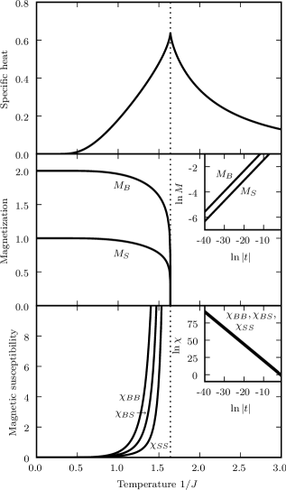
Figure 5: Specific heat, magnetizations, and zero-field magnetic susceptibilities for $p=0$, as functions of temperature $1/J$. The dotted vertical line marks the critical temperature $T_{c}=1.641$. As insets to the magnetizations and susceptibilities, we show $\ln M$ and $\ln\chi$ with respect to $\ln|t|$, where $t=\frac{T-T_{c}}{T_{c}}<0$. The linear behavior in the insets agrees with the power-law predictions of $M_{B}$, $M_{S}\sim|t|^{0.162}$ and $\chi_{BB}$, $\chi_{BS}$, $\chi_{SS}\sim|t|^{-2.353}$.

III.2 Critical Properties at $p=1$

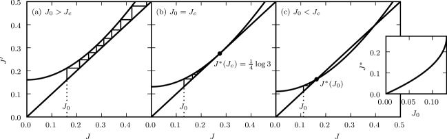
Figure 6: Three possible behaviors of the renormalization-group flows of the $p=1$ network with uniform long-range bonds. The curve in each diagram is the recursion $J^{\prime}(J)$ from Eq. (32), with the straight line $J^{\prime}=J$ also drawn for reference. Intersections of the curve with the straight line are fixed points. The flows are given by the staggered line, with successive values of $J^{\prime}$ corresponding to where the staggered line touches the curve. Only the dotted fixed points are physically accessible. The inset on the right shows the continuous line of fixed points $J^{\ast}(J_{0})$ as a function of $J_{0}$.

For the $p=1$ lattice, the renormalization-group transformation consists of decimating the two center sites in each connected cluster of the type shown on the top right of Fig. 1. The Hamiltonian now includes long-range bonds, Eq. (11), and the transformation is a mapping of the Hamiltonian $-\beta{\cal H}(J,H_{B},H_{S},\{K_{q}\},G)$ onto a renormalized Hamiltonian $-\beta^{\prime}{\cal H}^{\prime}(J^{\prime},H_{B}^{\prime},H_{S}^{\prime},\{K_{q}^{\prime}\},G^{\prime}))$. The recursion relations are

$$J^{\prime} =\frac{1}{2}\ln\left(R_{++}R_{--}/R_{+-}^{2}\right)+K_{1}\,,$$

$$H_{B}^{\prime} =\frac{1}{2}\ln\left(R_{++}/R_{--}\right)\,,\qquad H_{S}^{\prime}=H_{S}\,,$$

$$G^{\prime} =4G+\frac{1}{2}\ln\left(R_{++}R_{--}R_{+-}^{2}\right)\,,$$

$$K_{q}^{\prime} =K_{q+1}\,,\qquad q=1,2,\ldots\,,$$ (27)

where $R_{++}$, $R_{--}$, and $R_{+-}$ are as given in Eq. (15).

Long-range bonds as well as nearest-neighbor bonds now contribute to the internal energy $U$,

$$U=\frac{N_{\text{nn}}U_{\text{nn}}+\sum_{q=1}^{\infty}q^{-\sigma}N_{\text{ld},q}U_{\text{ld},q}}{N_{\text{nn}}+\sum_{q=1}^{\infty}N_{\text{ld},q}}\,,$$ (28)

where

$$U_{\text{nn}} =\frac{1}{N_{\text{nn}}}\sum_{\langle ij\rangle_{\text{nn}}}\langle s_{i}s_{j}\rangle=\frac{1}{N_{\text{nn}}}\frac{\partial}{\partial J}\ln Z\,,$$

$$U_{\text{ld},q} =\frac{1}{N_{\text{ld},q}}\sum_{\langle ij\rangle_{\text{ld},q}}\langle s_{i}s_{j}\rangle=\frac{1}{N_{\text{ld},q}}\frac{\partial}{\partial K_{q}}\ln Z\,.$$ (29)

Here $N_{\text{ld},q}=4^{-q}N_{\text{nn}}$ is the number of long-range bonds with $m_{ij}=q$. Since $K_{q}^{\prime}$ does not depend on $J$, $H_{B}$, or $H_{S}$, the thermodynamic densities and response functions in $\mathbf{V}=(1,U_{\text{nn}},M_{B},M_{S},\chi_{BB},\chi_{BS},\chi_{SS})$ still obey the recursion relation in Eq. (21) with a matrix $\overleftrightarrow{\mathbf{W}}$ of the same form as in Eq. (22). The densities $U_{\text{ld},q}$, on the other hand, have the recursion relation

$$U_{\text{ld},1} =b^{-d}U_{\text{nn}}^{\prime}\frac{N_{\text{nn}}}{N_{\text{ld},1}}\frac{\partial J^{\prime}}{\partial K_{1}}=U_{\text{nn}}^{\prime}\,,$$

$$U_{\text{ld},q} =b^{-d}U_{\text{ld},q-1}^{\prime}\frac{N_{\text{ld},q-1}}{N_{\text{ld},q}}\frac{\partial K_{q-1}^{\prime}}{\partial K_{q}}=U_{\text{ld},q-1}^{\prime}\quad(q>1)\,.$$ (30)

Thus $U_{\text{ld},q}=U_{\text{nn}}^{(q)}$, where $U_{\text{nn}}^{(q)}$ is the nearest-neighor density $U_{\text{nn}}$ in the system reached after $q$ renormalization-group transformations. Thus all the long-range bond densities $U_{\text{ld},q}$ are found by evaluating $U_{\text{nn}}$ along the renormalization-group trajectory. Eq. (28) can be rewritten as

$$U=\frac{3}{4}\left(U_{\text{nn}}+\sum_{q=1}^{\infty}q^{-\sigma}4^{-q}U_{\text{nn}}^{(q)}\right)\,,$$ (31)

where we have also used $N_{\text{nn}}+\sum_{q=1}^{\infty}N_{\text{ld},q}=\frac{4}{3}N_{\text{nn}}$. From Eq. (31) and the recursion relation for $U_{\text{nn}}$, the leading singularity in $U_{\text{nn}}$ is also the leading singularity in $U$. It is sufficient to calculate the singular behavior of $U_{\text{nn}}$ to obtain the critical properties of $U$ and of the specific heat $C$.

III.2.1 Long-distance bonds with uniform interaction strengths

We first consider the case with no distance dependence in the strengths of the long-range bonds, $\sigma=0$. Here $K_{q}=J_{0}$ for all $q$ and after any number of renormalization-group transformations, where $J_{0}$ is the value of $J$ in the original system. The recursion relation for $J$ in the closed subspace $H_{B}=H_{S}=0$ is

$$J^{\prime}=J_{0}+\ln(\cosh 2J)\,.$$ (32)

There are three types of behavior possible for the renormalization-group flows, as illustrated in Fig. 6. For $J_{0}$ greater than a critical value $J_{c}$ (Fig. 6(a)), the flows go to the ordered phase sink $J^{\ast}=\infty$. For $J_{0}\leq J_{c}$ (Fig. 6(b,c)) the flows go to a continuous line of fixed points $J^{\ast}(J_{0})$, with a distinct fixed point for each starting interaction $J_{0}$. When $J_{0}=J_{c}$ exactly, the $J^{\prime}(J)$ curve touches tangentially the straight line $J^{\prime}=J$ at $J^{\ast}(J_{c})$, as shown in Fig. 6(b). This fact allows us to solve for $J^{\ast}(J_{c})$ and $J_{c}$ exactly:

$$J^{\ast}(J_{c})=\frac{1}{4}\ln 3\,,\qquad J_{c}=\ln\frac{3^{3/4}}{2}\,.$$ (33)

Thus the system is conventionally ordered below the critical temperature $T_{c}=1/J_{c}=7.645$. To understand the novel high-temperature phase above $T_{c}$, we look at the recursion matrix $\overleftrightarrow{\mathbf{W}}^{\ast}$ evaluated along the line of fixed points, $J^{\ast}(J_{0})$ for $J_{0}\leq J_{c}$. The form of the matrix is as in Eq. (24), with $u=\tanh 2J^{\ast}(J_{0})$ and $v=1+\text{sech}^{2}\,2J^{\ast}(J_{0})$. Since $J^{\ast}(J_{0})$ has the maximum value of $(\ln 3)/4=0.275$ for $J_{0}=J_{c}$ and tends to zero as $J_{0}$ increases, $0\leq u\leq 1/2$, $7/4\leq v\leq 2$. The left eigenvector of $\overleftrightarrow{\mathbf{W}}^{\ast}$ with eigenvalue $b^{d}$ is

$$\mathbf{V}^{\ast}= (1,\,U_{\text{nn}}=\frac{u}{2-u},\,M_{B}=0,\,M_{S}=0,$$

$$\qquad\chi_{BB}=\infty,\,\chi_{BS}=\infty,\,\chi_{SS}=\infty)\,.$$ (34)

It follows that, in the high-temperature phase, $M_{B}=M_{S}=0$ and that the susceptibilities $\chi_{BB}$, $\chi_{BS}$, $\chi_{SS}$ are infinite. Because the renormalization-group flows go to a line of fixed points ending at the critical point $J^{\ast}(J_{c})$, the correlation length is infinite throughout the phase and the correlations have power-law decay, characteristics which are typically seen just at $T=T_{c}$. (In contrast, the low-temperature ordered phase has the usual exponential decay of correlations.) This type of behavior, with a transition between phases with finite and infinite correlation lengths, was first seen in the Berezinskii-Kosterlitz-Thouless phase transition Berezinskii ; KosterlitzThouless , though with an important difference: There the algebraic order was in the low-temperature phase, while here it is the high-temperature phase that has this feature.

We now turn to the critical behavior of the system in the ordered phase, as $T\to T_{c}$ from below. For small negative $t=(T-T_{c})/T_{c}=(J_{c}-J_{0})/J_{0}$, we have $J_{0}=J_{c}+\delta$, where $\delta=J_{c}|t|$. As can be seen from Fig.(6a), a renormalization-group flow starting at $J_{0}$ spends a large number of iterations in the vicinity of $J^{\ast}(J_{c})=(\ln 3)/4$, before escaping to the ordered phase sink at $J^{\ast}=\infty$. If $n_{0}$ is the number of iterations initially required to get $J$ close to $J^{\ast}(J_{c})$ and $n^{\ast}$ is the number of iterations where $J\approx J^{\ast}(J_{c})$, then as $\delta\to 0$, $n_{0}$ remains constant, while $n^{\ast}\to\infty$. The dependence of $n^{\ast}$ on $\delta$ (and hence on $|t|$) determines the critical singularities. For a typical critical point, $n^{\ast}\sim(\ln\delta)/(y_{T}\ln b)$. However, in our case, at $J^{\ast}(J_{c})$ the eigenvalue exponent $y_{T}=0$, and it turns out that $n^{\ast}\sim\delta^{-1/2}$. We show this as follows: After $n_{0}$ iterations, the flow is at $J$ near $J^{\ast}(J_{c})$, with $J<J^{\ast}(J_{c})$. It then takes $n^{\ast}/2$ iterations to get $J$ almost exactly at $J^{\ast}(J_{c})$, and another $n^{\ast}/2$ iterations to get $J$ a significant distance away from $J^{\ast}(J_{c})$, namely to $J-J_{c}\sim\text{O}(1)$. Considering the latter half of this flow, we expand the recursion relation for $J$, Eq. (32), around $J^{\ast}(J_{c})$,

$$J^{\prime}-J^{\ast}(J_{c})= ~{}\delta+(J-J^{\ast}(J_{c}))+\frac{3}{2}(J-J^{\ast}(J_{c}))^{2}$$

$$\qquad-(J-J^{\ast}(J_{c}))^{3}+\cdots\,.$$ (35)

Starting with $J=J^{\ast}(J_{c})$, from Eq. (35), we obtain series expressions for $J^{(i)}$, the interaction after $i$ renormalization-group steps:

$$J^{(1)}-J^{\ast}(J_{c}) =\delta$$

$$J^{(2)}-J^{\ast}(J_{c}) =2\delta+\frac{3}{2}\delta^{2}-\delta^{3}+\cdots$$

$$.\>.\>.$$

$$J^{(n)}-J^{\ast}(J_{c}) =n\delta+\frac{1}{4}(n-1)n(2n-1)\delta^{2}$$

$$+\frac{1}{80} (n-3)(n-1)n(24n^{2}-29n+2)\delta^{3}+\cdots$$ (36)

For $n\ll\delta^{-1/2}$, the first term in the series for $J^{(n)}-J^{\ast}(J_{c})$ is dominant, and the distance increases very slowly as $J^{(n)}-J^{\ast}(J_{c})\simeq n\delta$. For large $n$, the $k$th term in the series $\sim n^{2k-1}\delta^{k}$. Thus, when $n$ is of the order $\delta^{-1/2}$, $J^{(n)}-J^{\ast}(J_{c})$ begins to increase significantly. From this we can deduce that $n^{\ast}$ scales like $\delta^{-1/2}$.

We can now proceed to find the critical behaviors for the correlation length, thermodynamic densities, and response functions. By iterating the recursion relation for the correlation length, $\xi=b\xi^{\prime}$, $\xi=b^{n^{\ast}+n_{0}}\xi^{(n+n_{0})}$, where $\xi^{(n)}$ is the correlation length after $n$ renormalization-group steps. The singularity in $\xi$ as $\delta\to 0$ comes from the $b^{n^{\ast}}$ factor,

$$\xi\sim b^{n^{\ast}}\sim e^{\frac{C\ln 2}{\sqrt{\delta}}}=e^{\frac{A}{\sqrt{|t|}}}\,,$$ (37)

where $n^{\ast}\approx C\delta^{-1/2}$ for some constant $C$, and $A=C/\sqrt{J_{c}}$.

From Eqs. (22),(23), we extract the critical behaviors of the internal energy, magnetizations, and susceptibilities: The nearest-neighbor contribution to the internal energy $U_{\text{nn}}$ transforms as

$$U_{\text{nn}}=b^{-d}\frac{\partial G^{\prime}}{\partial J}+b^{-d}U_{\text{nn}}^{\prime}\frac{\partial J^{\prime}}{\partial J}\,.$$ (38)

Since $\partial G^{\prime}/\partial J$ is analytic, the singularity of $U_{\text{nn}}$ must reside in $U_{\text{nn}_{\text{\scriptsize sing}}}=b^{-d}U_{\text{nn}}^{\prime}\partial J^{\prime}/\partial J$. Iterating over $n_{0}+n^{\ast}$ renormalization-group steps,

$$U_{\text{nn}_{\text{\scriptsize sing}}} =b^{-(n_{0}+n^{\ast})d}U_{\text{nn}}^{(n_{0}+n^{\ast})}\prod_{i=1}^{n_{0}+n^{\ast}}\left.\frac{\partial J^{\prime}}{\partial J}\right|_{J=J^{(i)}}$$

$$\simeq b^{-n^{\ast}d}\left[b^{-n_{0}d}U_{\text{nn}}^{(n_{0}+n^{\ast})}\prod_{i=1}^{n_{0}}\left.\frac{\partial J^{\prime}}{\partial J}\right|_{J=J^{(i)}}\right]\,,$$ (39)

where we have used the fact that $\partial J^{\prime}/\partial J\simeq 1$ for the $n^{\ast}$ iterations during which $J^{(i)}\simeq J^{\ast}(J_{c})$. After $n+n^{\ast}$ iterations the system has flowed away from criticality. The singular dependence comes from the $b^{-n^{\ast}d}$ factor,

$$U_{\text{nn}_{\text{\scriptsize sing}}}\sim b^{-n^{\ast}d}\sim e^{-\frac{dA}{\sqrt{|t|}}}\,.$$ (40)

Thus the singular part of the specific heat is

$$C_{\text{\scriptsize sing}}\sim|t|^{-3/2}e^{-\frac{dA}{\sqrt{|t|}}}.$$ (41)

The magnetizations $M_{B}$ and $M_{S}$ recur as

$$(M_{B},M_{S}) =b^{-d}(M_{B}^{\prime},M_{S}^{\prime})\begin{pmatrix}2+2u&\frac{3}{2}u\\ 0&1\end{pmatrix}\,,$$ (42)

where $u=\tanh 2J$. Iterating over $n_{0}+n^{\ast}$ renormalization-group steps,

$$(M_{B},M_{S})$$

$$\>\simeq b^{-(n_{0}+n^{\ast})d}\left((M_{B}^{(n_{0}+n^{\ast})},M_{S}^{(n_{0}+n^{\ast})})\cdot\mathbf{v}\right)b^{n^{\ast}y_{H}}\mathbf{v}\cdot\mathbf{R}\,.$$ (43)

Here $b^{y_{H}}=2+2\tanh 2J^{\ast}(J_{c})=3$ is the largest eigenvalue of the $2\times 2$ derivative matrix in Eq. (42) evaluated at $J^{\ast}(J_{c})$, $\mathbf{v}$ is the corresponding normalized (to unity) eigenvector, and $\mathbf{R}$ is the product of the derivative matrices of the first $n_{0}$ iterations. The singular behavior comes from the factor $b^{-n^{\ast}(d-y_{H})}$,

$$M_{B},\,M_{S}\sim b^{-n^{\ast}(d-y_{H})}\sim e^{-\frac{(d-y_{H})A}{\sqrt{|t|}}}\,.$$ (44)

Since $y_{H}=1.585$, the magnetizations decrease exponentially to zero as $|t|\to 0$.

The susceptibilities $\chi_{BB}$, $\chi_{BS}$, and $\chi_{SS}$ recur as

$${\small(\chi_{BB},\chi_{BS},\chi_{SS})}$$

$${\small=b^{-d}(\chi_{BB}^{\prime},\chi_{BS}^{\prime},\chi_{SS}^{\prime})\begin{pmatrix}(2+2u)^{2}&\sqrt{6}u(1+u)&\frac{3u^{2}}{2}\\ 0&2+2u&\sqrt{\frac{3}{2}}u\\ 0&0&1\end{pmatrix}}$$

$${\small\qquad+b^{-d}(G^{\prime},U_{\text{nn}}^{\prime})\begin{pmatrix}4v&{\sqrt{6}}v&\frac{3v}{2}\\ -4u^{2}&\sqrt{6}u^{2}&-\frac{3u^{2}}{2}\end{pmatrix}\,,}$$ (45)

where $v=1+\text{sech}^{2}\,2J$. Since there is no singular behavior in $G^{\prime}$ and $U^{\prime}_{\text{nn}_{\text{\scriptsize sing}}}\to 0$ as $|t|\to 0$, only the first term in Eq. (45) contributes to the divergent singularity of the susceptibilities. Iterating over $n_{0}+n^{\ast}$ steps,

$$(\chi_{BB},\chi_{BS},\chi_{SS})_{\text{sing}}\sim b^{-(n_{0}+n^{\ast})d}$$

$$\>\left((\chi_{BB}^{(n_{0}+n^{\ast})},\chi_{BS}^{(n_{0}+n^{\ast})},\chi_{SS}^{(n_{0}+n^{\ast})})\cdot\mathbf{v}\right)b^{2n^{\ast}y_{H}}\mathbf{v}\cdot\mathbf{R}\,,$$ (46)

where $b^{2y_{H}}=(2+2\tanh 2J^{\ast}(J_{c}))^{2}$ is the largest eigenvalue of the $3\times 3$ derivative matrix in Eq. (45) evaluated at $J^{\ast}(J_{c})$, $\mathbf{v}$ the corresponding normalized eigenvector, and $\mathbf{R}$ the product of the derivative matrices for the first $n_{0}$ steps. The singularity in the susceptibilities is given by

$${\chi_{BB}}_{\text{sing}},\,{\chi_{BS}}_{\text{sing}},\,{\chi_{SS}}_{\text{sing}}\sim b^{n^{\ast}(2y_{H}-d)}\sim e^{\frac{(2y_{H}-d)A}{\sqrt{|t|}}}\,.$$ (47)

We illustrate these results in Fig. 7, plotting the specific heat, magnetizations, and zero-field susceptibilities as a function of temperature. The essential singularity in the specific heat (Eq. (41)) is invisible in the plot, the function and all its derivatives being continuous at $T_{c}$, with the rounded analytic peak occurring in the phase opposite to the algebraic phase, namely in the ordered phase at lower temperature. This behavior of the specific heat also occurs in the XY model undergoing a Berezinskii-Kosterlitz-Thouless phase transition, as seen in Fig. 5 of Ref.BerkerNelson . In the latter case, opposite to the algebraic phase, the phase in which the rounded analytic peak occurs is the disordered phase at higher temperature. In the XY model, the physical meaning of the high-temperature rounded peak is the onset of short-range order within the disordered phase. In our current system, the physical meaning of the low-temperature rounded peak is the saturation of long-range order that occurs unusually away from criticality, due to the essential critical singularity of the magnetization, which corresponds to a critical exponent $\beta=\infty$ and the unusual flat onset of the magnetization, as seen in Fig. 7.

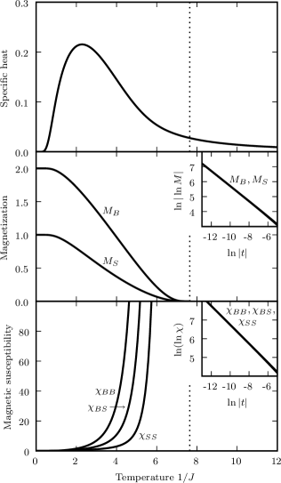
Figure 7: Specific heat, magnetizations, and magnetic susceptibilities for $p=1$ long-range bonds with uniform interaction strengths ($\sigma=0$), as a function of temperature $1/J$. The dotted vertical line marks the critical temperature $T_{c}=7.645$. The insets to the magnetization and susceptibility graphs show $\ln|\ln M|$ and $\ln(\ln\chi)$ versus $\ln|t|$, where $t=\frac{T-T_{c}}{T_{c}}<0$. The linear behavior in the insets agrees with the exponential scaling predictions of $M_{B}$, $M_{S}\sim e^{-C/\sqrt{|t|}}$ and $\chi_{BB}$, $\chi_{BS}$, $\chi_{SS}\sim e^{D/\sqrt{|t|}}$ with positive constants $C$ and $D$ .

III.2.2 Long-distance bonds with decaying interaction strengths

For $\sigma>0$, the long-range bond strengths $K_{q}=J_{0}q^{-\sigma}$ and thus at the $n$th renormalization-group step $K_{1}^{(n)}=J_{0}(n+1)^{-\sigma}$. The interaction strength $J^{(n)}$ in the closed subspace $H_{B}=H_{S}=0$ is given by the recursion relation

$$J^{(n)}=J_{0}n^{-\sigma}+\ln(\cosh 2J^{(n-1)})\,,$$ (48)

where $J^{(0)}=J_{0}$. The critical temperature $T_{c}$ now depends on the exponent $\sigma$, as shown in top curve of Fig. 8, having the maximum value of $T_{c}=7.645$ at $\sigma=0$ and decreasing with increasing $\sigma$ (to $T_{c}=2.744$ at $\sigma=\infty$, where the system reduces to a nearest-neighbor, next-nearest-neighbor model).

When the number of renormalization-group steps $n\to\infty$, the $J_{0}n^{-\sigma}$ term in Eq. (48) goes to zero, so that the fixed points of the renormalization-group transformation are those of the $p=0$ case analyzed in Sec. III.A. Thus for temperatures close enough to $T_{c}$, satisfying $|t|\ll\tau$ for some crossover value $\tau$, we expect to observe the $p=0$ critical behavior. However, the width $\tau$ of the critical region varies with $\sigma$, becoming extremely narrow as $\sigma\to 0$. For a thermodynamic quantity scaling as $|t|^{x}$ inside the critical region ($x$ being one of the $p=0$ exponents), the general scaling behavior for small $|t|$ not necessarily in the critical region is $|t|^{x+f_{x}(t)}$, where $|f_{x}(t)|\ll|x|$ when $|t|\ll\tau$, and the form of $f_{x}(t)$ may depend on $\sigma$. In the following, we derive the leading order contribution to $f_{x}(t)$ for the various physical properties of the system, also determining the size of the critical region $\tau$.

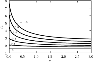
Figure 8: Critical temperature $T_{c}=1/J_{c}$ for various $p$ as a function of the exponent $\sigma$ describing the decay of the long-range bond interaction strengths. The curves for $0<p<1$ were calculated using the techniques in Section III.C.

If the system is at its critical temperature, $J_{0}=J_{c}$, the interaction strength under repeated renormalization-group iterations, $J^{(n)}$ for $n\to\infty$, goes to the $p=0$ critical fixed point, which we will label $J_{c0}$ and whose value is given by Eq. (16). Let us denote this renormalization-group flow as $J_{c}^{(n)}$, so that $J_{c}^{(0)}=J_{c}$ and $\lim_{n\to\infty}J_{c}^{(n)}=J_{c0}$. Now if we start instead at a temperature very close to critical, $J_{0}=J_{c}-J_{c}t$ for small $|t|$, $J^{(n)}$ stays near $J^{(n)}_{c}$ for a large number of iterations $n^{\ast}$, before veering off to either the ordered or disordered sink. The dependence of $n^{\ast}$ on $|t|$ is the key to the crossover behavior of the system. The difference $J^{(n)}-J_{c}^{(n)}$ satisfies the recursion relation

$$J^{(n+1)}-J_{c}^{(n+1)}=b^{y_{T}(n)}(J^{(n)}-J_{c}^{(n)})\,,$$ (49)

where

$$b^{y_{T}(n)}=\left.\frac{\partial J^{(n+1)}}{\partial J^{(n)}}\right|_{J^{(n)}=J_{c}^{(n)}}=2\tanh 2J_{c}^{(n)}\,.$$ (50)

Iterating Eq. (49),

$$J^{(n+1)}-J_{c}^{(n+1)} =b^{\sum_{k=0}^{n}y_{T}(k)}(J_{0}-J_{c})$$

$$=b^{\sum_{k=0}^{n}y_{T}(k)}(-J_{c}t)\,.$$ (51)

Since $J^{(n^{\ast})}-J_{c}^{(n^{\ast})}\sim\text{O}(1)$,

$$b^{\sum_{k=0}^{n^{\ast}}y_{T}(k)}\sim|t|^{-1}\ \quad\text{and}\quad\sum_{k=0}^{n^{\ast}}y_{T}(k)\sim-\frac{\ln|t|}{\ln b}\,.$$ (52)

In order to find $n^{\ast}$, we need to determine $y_{T}(n)$. From the fact that $\lim_{n\to\infty}J_{c}^{(n)}=J_{c0}$ and the recursion relation in Eq. (48), we consider for $J_{c}^{(n)}$ the large $n$ form of

$$J_{c}^{(n)}=J_{c0}-Bn^{-\sigma}+\cdots\,.$$ (53)

Substitution into Eq. (48) yields

$$B=\frac{J_{0}}{2\tanh 2J_{c0}-1}\,.$$ (54)

Eqs. (53),(54) can also be obtained by expanding the recursion relation around $J_{c0}$,

$$J_{c}^{(n)}-J_{c0}=J_{0}n^{-\sigma}+2\tanh 2J_{c0}(J_{c}^{(n-1)}-J_{c0})\,,$$ (55)

and summing the series derived from iterating Eq. (55). Substituting into Eq. (50),

$$y_{T}(n)=y_{T0}-Cn^{-\sigma}+\cdots\,,$$ (56)

where $y_{T0}=\ln(2\tanh 2J_{c0})/\ln b=0.747$ is the $p=0$ thermal eigenvalue exponent and $C=1.498J_{0}$. For use below, we also deduce the magnetic exponents $y_{H}(n)$,

$$b^{y_{H}(n)} =\left.\frac{\partial H_{B}^{(n+1)}}{H_{B}^{(n)}}\right|_{J^{(n)}=J_{c}^{(n)},H_{B}^{(n)}=H_{S}^{(n)}=0}$$

$$=2+2\tanh 2J^{(n)}_{c},$$

$$y_{H}(n) =y_{H0}-Dn^{-\sigma}+\cdots\,.$$ (57)

where $y_{H0}=\ln(2+2\tanh 2J_{c0})/\ln b=1.879$ is the $p=0$ magnetic eigenvalue exponent and $D=0.683J_{0}$.

From Eq. (56), we evaluate $\sum_{k=0}^{n^{\ast}}y_{T}(k)$ for large $n^{\ast}$,

$$\sum_{k=0}^{n^{\ast}}y_{T}(k)\simeq\begin{cases}n^{\ast}y_{T0}-\frac{C{n^{\ast}}^{1-\sigma}}{1-\sigma}\,,&0<\sigma<1\,,\\ n^{\ast}y_{T0}-C\ln n^{\ast},&\sigma=1\,,\\ n^{\ast}y_{T0}-C\zeta(\sigma)\,,&\sigma>1\,.\end{cases}$$ (58)

For $\sigma\geq 1$, the $n^{\ast}y_{T0}$ term is clearly dominant for large $n^{\ast}$, so that, from Eq. (52),

$$n^{\ast}\simeq-\frac{1}{y_{T0}}\frac{\ln{|t|}}{\ln b}\equiv n^{\ast}_{0}\qquad(\sigma\geq 1)\,.$$ (59)

This expression for $n^{\ast}$ leads to the same critical exponents we found in the $p=0$ case. On the other hand, for the slow decay of $0<\sigma<1$, Eq. (52) becomes

$$n^{\ast}y_{T0}-\frac{C{n^{\ast}}^{1-\sigma}}{1-\sigma}\simeq-\frac{\ln|t|}{\ln b}\,.$$ (60)

Writing $n^{\ast}=n^{\ast}_{0}+\delta n$, the leading order contribution to $\delta n$ is found,

$$n^{\ast}=n^{\ast}_{0}+\frac{C{n^{\ast}_{0}}^{1-\sigma}}{(1-\sigma)y_{T0}}+\cdots\qquad(0<\sigma<1)\,.$$ (61)

This expression for $n^{\ast}$ when $0<\sigma<1$ yields the leading-order corrections to $p=0$ in the critical behaviors of the correlation length, internal energy, specific heat, magnetizations, and susceptibilities:

$$\xi \sim b^{n^{\ast}}\sim|t|^{-\frac{1}{y_{T0}}-\frac{C}{(1-\sigma)y_{T0}^{2-\sigma}}\left(-\frac{\ln|t|}{\ln b}\right)^{-\sigma}}\,,$$

$$U_{\text{sing}} \sim b^{-n^{\ast}d+\sum_{k=0}^{n^{\ast}}y_{T}(k)}$$

$$\sim|t|^{\frac{d-y_{T0}}{y_{T0}}+\frac{dC}{(1-\sigma)y_{T0}^{2-\sigma}}\left(-\frac{\ln|t|}{\ln b}\right)^{-\sigma}}\,,$$

$$C_{\text{sing}} \sim|t|^{\frac{d-2y_{T0}}{y_{T0}}+\frac{dC}{(1-\sigma)y_{T0}^{2-\sigma}}\left(-\frac{\ln|t|}{\ln b}\right)^{-\sigma}}\,,$$

$$M_{B},\,M_{S} \sim b^{-n^{\ast}d+\sum_{k=0}^{n^{\ast}}y_{H}(k)}$$

$$\sim|t|^{\frac{d-y_{H0}}{y_{T0}}+\frac{(d-y_{H0})C+y_{T0}D}{(1-\sigma)y_{T0}^{2-\sigma}}\left(-\frac{\ln|t|}{\ln b}\right)^{-\sigma}}\,,$$

$$\chi_{BB},\,\chi_{BS},\,\chi_{SS} \sim b^{-n^{\ast}d+2\sum_{k=0}^{n^{\ast}}y_{H}(k)}$$

$$\sim|t|^{\frac{d-2y_{H0}}{y_{T0}}+\frac{(d-2y_{H0})C+2y_{T0}D}{(1-\sigma)y_{T0}^{2-\sigma}}\left(-\frac{\ln|t|}{\ln b}\right)^{-\sigma}}\,.$$ (62)

All the critical behavior expressions in Eqs. (62) have the form $|t|^{x+\frac{E}{(1-\sigma)y_{T0}^{2-\sigma}}\left(-\frac{\ln|t|}{\ln b}\right)^{-\sigma}}$, where $x$ is the appropriate $p=0$ exponent and $E$ is a non-universal (i.e., $J_{0}$-dependent) constant $\sim\text{O(1)}$. For temperatures $|t|<\tau$, the leading-order correction term in the exponent should be negligible,

$$\frac{1}{(1-\sigma)y_{T0}^{2-\sigma}}\left(-\frac{\ln|t|}{\ln b}\right)^{-\sigma}\lesssim\epsilon\,,$$ (63)

for some small quantity $\epsilon$, giving an estimate for $\tau$ as $\sigma\to 0$,

$$\tau\approx b^{-\left(\epsilon(1-\sigma)y_{T0}^{2-\sigma}\right)^{-1/\sigma}}\,.$$ (64)

With decreasing $\sigma$ the critical region $\tau$ becomes rapidly infinitesimal. For example, with $\sigma=1/2$ and $\epsilon=10^{-1}$, $\tau\approx 10^{-289}$.

The above corrections to critical behavior are illustrated in Fig. 9, where we plot numerically calculated effective exponents $\ln M_{BB}/\ln|t|$ and $\ln\chi_{BB}/\ln|t|$ as a function of $|t|$ for several values of $\sigma$. It is clear that for $\sigma\geq 1$, the effective exponents quickly converge to the horizontal lines showing the actual asymptotic exponents. The convergence when $\sigma<1$ is much slower, due to the $|t|^{\frac{E}{(1-\sigma)y_{T0}^{2-\sigma}}\left(-\frac{\ln|t|}{\ln b}\right)^{-\sigma}}$ correction to asymptotic universal critical behavior. In Fig. 10 we explicitly show for the case $\sigma=0.6$ the magnetizations and susceptibilities asymptotically approaching the scaling forms of Eq. (62) for small $|t|$.

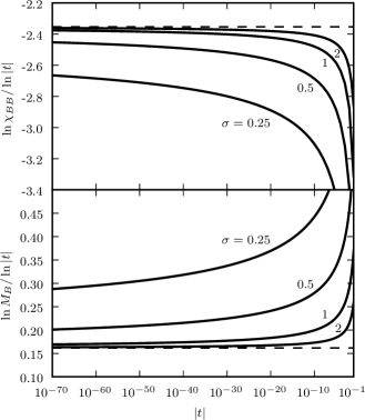
Figure 9: The calculated effective exponent of the magnetization $M_{B}$ and magnetic susceptibility $\chi_{BB}$, as a function of $|t|$ for $t=\frac{T-T_{c}}{T_{c}}<0$ and $p=1$. Curves for several values of $\sigma$, the exponent for the decay of the long-range bond strengths, are shown. The horizontal dashed line in the upper graph corresponds to the actual critical exponent for the susceptibility, $-\gamma=-(2y_{H0}-d)/y_{T0}=-2.353$, while the dashed line in the lower graph corresponds to the actual magnetization exponent, $\beta=(d-y_{T0})/y_{T0}=0.162$.

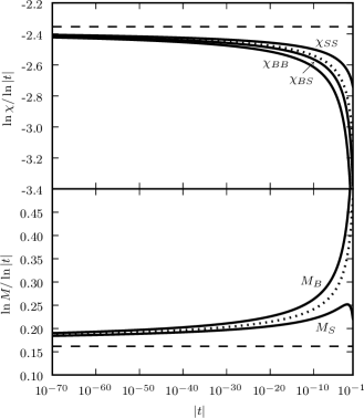
Figure 10: The effective exponents of the magnetizations $M_{B}$ and $M_{S}$, and susceptibilities $\chi_{BB}$, $\chi_{BS}$, and $\chi_{SS}$, for $p=1$, $\sigma=0.6$, plotted as a function of $|t|$ for $t=\frac{T-T_{c}}{T_{c}}<0$. The dotted curves in the figures are the first-correction-to-scaling predictions for the magnetization and susceptibility from Eq. (62). The horizontal dashed line in the upper graph corresponds to the $p=0$ critical exponent for the susceptibility, $-\gamma=-(2y_{H0}-d)/y_{T0}=-2.353$, while the dashed line in the lower graph corresponds to the $p=0$ magnetization exponent, $\beta=(d-y_{T0})/y_{T0}=0.162$.

III.3 Critical Properties of the System with Long-Range Quenched Randomness, $0<p<1$

III.3.1 Exact renormalization-group transformation for quenched probability distributions

When $0<p<1$, there is long-range quenched randomness in the network, and the renormalized system will have an inhomogenous distribution of all interaction constants. The renormalization-group transformation needs be formulated in terms of quenched probability distributions AndelmanBerker . First consider the decimation transformation effected on the cluster of Fig. 11, with nonuniform interaction constants. The recursion relations for ${J^{\prime}}_{i^{\prime}j^{\prime}}$, ${H_{B}^{\prime}}_{i^{\prime}j^{\prime}}$, $H_{S}^{\prime}$, and $G^{\prime}_{i^{\prime}j^{\prime}}$ are the locally differentiated versions of Eq. (27),

$$J^{\prime}(i^{\prime}j^{\prime}) =J^{\prime}(i^{\prime}k_{1}j^{\prime})+J^{\prime}(i^{\prime}k_{2}j^{\prime})+K_{1}(i^{\prime}j^{\prime})\,,$$

$$J^{\prime}(i^{\prime}k_{1}j^{\prime})=\frac{1}{4}\ln\left(R_{++}R_{--}/R_{+-}^{2}\right)_{(i^{\prime}k_{1}j^{\prime})}\,,$$

$$H_{B}^{\prime}(i^{\prime}j^{\prime}) =H_{B}^{\prime}(i^{\prime}k_{1}j^{\prime})+H_{B}^{\prime}(i^{\prime}k_{2}j^{\prime}),\quad H_{S}^{\prime}(i^{\prime})=H_{S}(i^{\prime})\,,$$

$$H_{B}^{\prime}(i^{\prime}k_{1}j^{\prime})=\frac{1}{4}\ln\left(R_{++}/R_{--}\right)_{(i^{\prime}k_{1}j^{\prime})}\,,$$

$$G^{\prime}(i^{\prime}j^{\prime}) =G^{\prime}(i^{\prime}k_{1}j^{\prime})+G^{\prime}(i^{\prime}k_{2}j^{\prime})\,,$$

$$G^{\prime}(i^{\prime}k_{1}j^{\prime})=\frac{1}{4}\ln\left(R_{++}R_{--}R_{+-}^{2}\right)_{(i^{\prime}k_{1}j^{\prime})}\,,$$

$$K_{q}^{\prime} =K_{q+1}\,,\qquad q=1,2,\ldots\,,$$ (65)

where $R_{++}$, $R_{--}$, and $R_{+-}$ along path $(i^{\prime}kj^{\prime})$ are given by the locally differentiated versions of Eq. (15),

$$R_{++} =x_{1}x_{2}y_{1}y_{2}z+x_{1}^{-1}x_{2}^{-1}z^{-1}\,,$$

$$R_{--} =x_{1}^{-1}x_{2}^{-1}z+x_{1}x_{2}y_{1}^{-1}y_{2}^{-1}z^{-1}\,,$$

$$R_{+-} =x_{1}x_{2}^{-1}y_{1}z+x_{1}^{-1}x_{2}y_{2}^{-1}z^{-1}\,,$$

$$x_{1}=e^{J(i^{\prime}k)},\,x_{2}=e^{J(kj^{\prime})}\,,$$

$$y_{1}=e^{2H_{B}(i^{\prime}k)},\,y_{2}=e^{2H_{B}(kj^{\prime})},\,z=e^{H_{S}(k)}.$$ (66)

If there is no long-range bond connecting $i^{\prime}$ and $j^{\prime}$, the equations above hold with $K_{1}(i^{\prime}j^{\prime})=0$. We shall work in the closed subspace $H_{B}(ij)=H_{S}(i)=0$ for all $i$,$j$, where the recursion relation for $J^{\prime}(i^{\prime}j^{\prime})$ is a function

$$J^{\prime}(i^{\prime}j^{\prime})=R(\{J(ij)\};K_{1}(i^{\prime}j^{\prime}))\,,$$ (67)

with $\{J(ij)\}=\{J(i^{\prime}k_{1}),J(k_{1}j^{\prime}),J(i^{\prime}k_{2}),J(k_{2}j^{\prime})\}$ being the set of interaction constants in the cluster, and $R$ given in Eqs. (65) and (66).

If the interaction constants $J(ij)$ have a quenched probability distribution ${\cal P}(J(ij))$, and the long-range bonds $K_{q}(ij)$ have a quenched probability distribution ${\cal Q}^{(q)}(K_{q}(ij))$, the distribution ${\cal P}^{(n)}(J^{\prime}_{i^{\prime}j^{\prime}})$ for the rescaled system after $n$ renormalization-group transformations is given by the convolution

$${\cal P}^{(n)}(J^{\prime}(i^{\prime}j^{\prime}))=$$

$$\int\Bigl{[}\prod_{ij}^{i^{\prime}j^{\prime}}dJ(ij){\cal P}^{(n-1)}(J(ij))\Bigr{]}dK_{1}(i^{\prime}j^{\prime}){\cal Q}^{(n-1)}(K_{1}(i^{\prime}j^{\prime}))$$

$$\qquad\qquad\delta\left(J^{\prime}(i^{\prime}j^{\prime})-R(\{J_{ij}\};K_{1}(i^{\prime}j^{\prime})\right)\,,$$ (68)

where the product runs over the nearest-neighbor bonds $ij$ in the cluster between $i^{\prime}$ and $j^{\prime}$. The long-range bond distribution ${\cal Q}^{(n)}(K^{\prime}_{1}(i^{\prime}j^{\prime}))$ after $n$ renormalization-group transformations is

$${\cal Q}^{(n)}(K^{\prime}_{1}(i^{\prime}j^{\prime})) =p\,\delta\left(K^{\prime}_{1}(i^{\prime}j^{\prime})-J_{0}(n+1)^{-\sigma}\right)$$

$$\qquad+(1-p)\delta\left(K^{\prime}_{1}(i^{\prime}j^{\prime})\right)\,.$$ (69)

Figure 11: Cluster with quenched randomness on which the decimation transformation of Eq. (65) is applied.

The convolution in Eq. (68) is implemented numerically, with the probability distribution ${\cal P}^{(n)}(J_{ij})$ represented by histograms, each histogram consisting of a bond strength and its associated probability. The initial distribution ${\cal P}^{(0)}(J_{ij})$ is a single histogram at $J_{0}$ with probability $1$. Since Eq. (68) is a convolution of five probability distributions, computational storage limits can be used most effectively by factoring it into an equivalent series of three pairwise convolutions, each of which involves only two distributions convoluted with an appropriate $R$ function. Two types of pairwise convolutions are required, a “bond-moving” convolution with

$$R_{\text{bm}}(J(i_{1}j_{1}),J(i_{2}j_{2}))=J(i_{1}j_{1})+J(i_{2}j_{2})\,,$$ (70)

and a decimation convolution with

$$R_{\text{dc}}(J(i_{1}j_{1}),J(i_{2}j_{2}))=\frac{1}{2}\ln\left(\frac{\cosh(J(i_{1}j_{1})+J(i_{2}j_{2}))}{\cosh(J(i_{1}j_{1})-J(i_{2}j_{2}))}\right)\,.$$ (71)

Starting with the probability distribution ${\cal P}^{(n-1)}$, the following series of pairwise convolutions gives the total convolution of Eq. (68): (i) a decimation convolution of ${\cal P}^{(n-1)}$ with itself, yielding ${\cal P}_{A}$; (ii) a bond-moving convolution of ${\cal P}_{A}$ with itself, yielding ${\cal P}_{B}$; (iii) a bond-moving convolution of ${\cal P}_{B}$ with ${\cal Q}^{(n-1)}$, yielding the final result ${\cal P}^{(n)}$.

Because the number of histograms representing the probability distribution increases rapidly with each renormalization-group step, we use a binning procedure FalicovBerkerMcKay : before every pairwise convolution, the histograms are placed on a grid, and all histograms falling into the same grid cell are combined into a single histogram in such a way that the average and the standard deviation of the probability distribution are preserved. Histograms falling outside the grid, representing a negligible part of the total probability, are similarly combined into a single histogram. Any histogram within a small neighborhood of a cell boundary is proportionately shared between the adjacent cells. After the convolution, the original number of histograms is reattained. For the results presented below we used 562,500 bins, requiring the calculation of 562,500 local renormalization-group transformations at every iteration.

For the thermodynamic densites $M_{\alpha}$, given by

$$M_{\alpha}=\frac{1}{N_{\alpha}}\sum_{ij}\frac{\partial\ln Z}{\partial K_{\alpha}(ij)}\,,$$ (72)

the chain rule yields conjugate recursion relations for the quenched random system,

$$M_{\alpha}=b^{-d}\sum_{\beta}\frac{1}{N^{\prime}_{\beta}}\sum_{i^{\prime}j^{\prime}}\frac{\partial\ln Z}{\partial K^{\prime}_{\beta}(i^{\prime}j^{\prime})}\,\sum^{i^{\prime}j^{\prime}}_{ij}\frac{N_{\beta}}{N_{\alpha}}\frac{\partial K^{\prime}_{\beta}(i^{\prime}j^{\prime})}{\partial K_{\alpha}(ij)}\,,$$ (73)

where the rightmost sum runs over nearest-neighbor bonds $ij$ in the cluster between sites $i^{\prime}$ and $j^{\prime}$. As an approximation, this sum is replaced by its average value, so that

$$M_{\alpha}\approx b^{-d}\sum_{\beta}M_{\beta}^{\prime}\overline{T}_{\beta\alpha}\quad\text{with}\quad\overline{T}_{\beta\alpha}\equiv\sum^{i^{\prime}j^{\prime}}_{ij}\frac{N_{\beta}}{N_{\alpha}}\overline{\frac{\partial K^{\prime}_{\beta}(i^{\prime}j^{\prime})}{\partial K_{\alpha}(ij)}}\,,$$ (74)

Here the overbar denotes averaging over the probability distributions of the interaction constants in the cluster shown in Fig. 11. Using the recursion relations in Eq. (65), in the subspace ${H_{B}}_{ij}=H_{S}=0$,

$$\overline{\mathbf{T}} =\overline{\begin{pmatrix}4&\sum^{i^{\prime}j^{\prime}}_{ij}{\frac{\partial G^{\prime}(i^{\prime}j^{\prime})}{\partial J(ij)}}&0&0\\ 0&\sum^{i^{\prime}j^{\prime}}_{ij}{\frac{\partial J^{\prime}(i^{\prime}j^{\prime})}{\partial J(ij)}}&0&0\\ 0&0&\sum^{i^{\prime}j^{\prime}}_{ij}{\frac{\partial H^{\prime}_{B}(i^{\prime}j^{\prime})}{\partial H_{B}(ij)}}&\sum^{i^{\prime}j^{\prime}}_{i}{\frac{\partial H^{\prime}_{B}(i^{\prime}j^{\prime})}{\partial H_{S}(i)}}\\ 0&0&0&\sum^{i^{\prime}}_{i}{\frac{\partial H^{\prime}_{S}(i^{\prime})}{\partial H_{S}(i)}}\end{pmatrix}}$$

$$=\begin{pmatrix}4&2\overline{u}&0&0\\ 0&2\overline{u}&0&0\\ 0&0&2+2\overline{u}&{\frac{3\overline{w}}{2}}\\ 0&0&0&1\end{pmatrix}\,,$$ (75)

where

$$u =\frac{1}{2}(\tanh(J(i^{\prime}k_{1})+J(k_{1}j^{\prime}))$$

$$\qquad\qquad+\tanh(J(i^{\prime}k_{2})+J(k_{2}j^{\prime}))),$$

$$w =\frac{\sinh(J(i^{\prime}k_{1})+J(k_{1}j^{\prime})+J(i^{\prime}k_{2})+J(k_{2}j^{\prime}))}{2\cosh(J(i^{\prime}k_{1})+J(k_{1}j^{\prime}))\cosh(J(i^{\prime}k_{2})+J(k_{2}j^{\prime}))}\,.$$ (76)

For a fixed probability distribution of the renormalization-group transformation (e.g., Fig. 13), the thermal and magnetic eigenvalues exponents $y_{T}$ and $y_{H}$ are obtained as

$$b^{y_{T}} =\sum^{i^{\prime}j^{\prime}}_{ij}\overline{{\frac{\partial J^{\prime}(i^{\prime}j^{\prime})}{\partial J(ij)}}}=2\overline{u}\,,$$

$$b^{y_{H}} =\sum^{i^{\prime}j^{\prime}}_{ij}\overline{\frac{\partial H^{\prime}_{B}(i^{\prime}j^{\prime})}{\partial H_{B}(ij)}}=2+2\overline{u}\,.$$ (77)

III.3.2 Results

Figure 12: Critical temperature $T_{c}$ as a function of the probability of long-range bonds $p$, plotted for several values of the exponent $\sigma$ characterizing the decay of the long-range bond strengths.

Figure 13: Histograms of the unstable critical fixed probability distributions for $p=0.2$, $\sigma=0$ (left column) and $p=0.7$, $\sigma=0$ (right column). The bottom panels show the actual histograms (numbering 1,128,002 in each case), while in the top panels the histograms are combined in order to clearly see the outlines of the probability distributions.

Figure 14: The thermal and magnetic eigenvalues $y_{T}$ and $y_{H}$, and the corresponding specific heat and magnetic exponents $\alpha$ and $\beta$, as a function of $p$, for $\sigma=0$. The probability $p=0.494$, marking the onset of exponentiated power-law critical behavior, is shown with a dotted line.

Figure 15: Specific heat calculated for various probabilities $p$, plotted with respect to the normalized temperature $(T-T_{c})/T_{c}$, with $\sigma=0$. The vertical dotted line corresponds to the critical temperature $T=T_{c}$. The inset shows a close-up of the specific heat near $T_{c}$ for $p=0.06$, showing both the infinite-slope singularity at $T=T_{c}$, and the analytic peak that appears for $T<T_{c}$ when $p\gtrsim 0.053$.

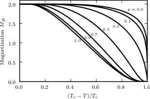
Figure 16: Magnetization calculated for various probabilities $p$, plotted with respect to the normalized temperature variable $(T_{c}-T)/T_{c}$, with $\sigma=0$. For $p>0.363$, note the unusual flat onset at $T_{c}$.

The quenched random system critical temperatures $T_{c}(p)=J^{-1}_{c}(p)$ are shown as a function of $p$, in Fig. 12, for several values of the decay exponent $\sigma$. For any $\sigma>0$, in renormalization-group trajectories starting near $T_{c}$, the probability distribution ${\cal P}(J(ij))$ spends many iterations in the vicinity of the unstable critical fixed distribution which is a delta function at $J_{c}(p=0)$, the $p=0$ critical interaction strength given by Eq. (16). Similarly to the results of the $p=1$ case given above, when $\sigma>0$, the critical behavior for all $p$ is that of $p=0$, though with a rapidly decreasing critical region as $p\to 1$ and $\sigma\to 0$.

On the other hand, for $\sigma=0$, a variety of critical behaviors occurs as $p$ ranges from 0 to 1. The unstable critical fixed distribution has a non-trivial structure which depends on $p$, two examples of which are shown in Fig. 13. The eigenvalue exponents $y_{T}$ and $y_{H}$ from the critical fixed distributions change continuously with $p$ (Fig. 14), and with them the critical exponents characterizing the phase transition. As $p$ is increased from zero, both $y_{T}$ and $y_{H}$ decrease from their $p=0$ values, attaining their $p=1$ values of $y_{T}=0$ and $y_{H}=\ln 3/\ln 2$ at $p=0.494$. Thus, the system has two distinct regimes of criticalities. For $p<0.494$ the critical behavior is described by power laws with exponents $\nu=1/y_{T}$, $\alpha=(2y_{T}-d)/y_{T}$, $\beta=(d-y_{H})/y_{T}$, and $\gamma=(2y_{H}-d)/y_{T}$. As $y_{T}\to 0$ with $p\to 0.494$, the exponents blow up as $\nu\to\infty$, $\alpha\to-\infty$, $\beta\to\infty$, and $\gamma\to\infty$. For $p\geq 0.494$ the critical behavior is that of the $p=1,\sigma=0$ case given above, with exponentiated power laws of the thermodynamic quantities, and the high-temperature phase has infinite correlation length. The onset of exponentiated power-law critical behavior at $p=0.494$, due to the influence of the long-range bonds, in fact corresponds to a change in the geometrical features of the network. As we have noted in Fig. 4, for $p\gtrsim 0.5$ the average path length $\ell$ has a small world character, $\ell\sim\ln N_{n}$, while for smaller $p$ it increases more rapidly like $N^{1/d}_{n}$, as in a regular lattice.

The spectrum of critical behaviors for varying $p$ at $\sigma=0$ is illustrated in Figs. 15 and 16 for the specific heat and magnetization versus temperature for different values of $p$. With increasing $p$ from $p=0$, the low-temperature analytic peak, due to the saturation of long-range order, as mentioned above, appears at $p\approx 0.053$, as the low-temperature amplitude of the critical cusp changes sign, and shifts to lower temperatures as $p$ further increases. At the critical-point singularity, with increasing $p$ from $p=0$, the specific heat exponent $\alpha$ continuously decreases from its $p=0$ value of $-0.677$: The cusp disappears at $p=0.105$ as $\alpha$ crosses $-1$, so that the specific heat acquires a continuous slope at criticality, but all higher derivatives remain divergent. The second derivative at criticality also becomes continuous, all higher derivatives remaining divergent, at $p=0.249$ as $\alpha$ crosses $-2$. Thus, as $\alpha$ crosses the consecutive negative integers at at $p=0.105$, $0.249$, $0.312$, $0.349,\ldots$, the divergence begins at a higher derivative, until the accumulation point at $p=0.494$, where $\alpha$ reaches $-\infty$, and the essential singularity occurs for the higher values of $p$.

In the magnetization, with increasing $p$ from $p=0$, the critical exponent $\beta$ continuously increases from its $p=0$ value of $0.162$. Thus, the slope at criticality changes from infinity to zero at $p=0.363$ as $\beta$ crosses $1$, but all higher derivatives of the magnetization remain divergent. The second derivative at criticality also becomes zero, all higher derivatives remaining divergent, at $p=0.424$ as $\beta$ crosses $2$. At each crossing of a positive integer by $\beta$, at $p=0.363$, $0.424$, $0.446$, $0.457,\ldots$, the zeros extend to one higher derivative and the divergence begins at one higher derivative, until the accumulation point at $p=0.494$, where $\beta$ reaches $\infty$, and the essential singularity occurs for the higher values of $p$.

IV Conclusions

In summary, we have introduced a scale-free hierarchical-lattice network model exhibiting a range of geometric and thermodynamic properties as we vary the probability $p$ of the long-distance bonds. When $p=0$, our network is unclustered and the average shortest-path length $\ell$ scales like a power-law in the number of sites, $\ell\sim N^{1/2}$, resembling in these respects a regular lattice. This resemblance also holds for the critical behavior of the ferromagnetic Ising model on the $p=0$ network, which shows typical power-law singularities in specific heat, magnetization, and susceptibility. For small concentrations of long-distance bonds, $p<0.494$, this picture does not change radically: the clustering coefficient increases nearly linearly with $p$, the average shortest-path length continues to have power-law scaling with lattice size, and the critical exponents of the Ising model vary continuously with $p$. As we approach $p=0.494$, however, the magnitudes of these exponents blow up, and we have an unexpected crossover to a completely different regime of critical behavior for $p\geq 0.494$. We find a highly unusual infinite-order phase transition, an inverted Berezinskii-Kosterlitz-Thouless singularity between a low-temperature phase with nonzero magnetization and finite correlation length, and a high-temperature phase with zero magnetization but infinite correlation length and power-law decay of correlations throughout the phase. This slow decay of correlations in the disordered phase is a direct consequence of the underlying lattice topology, since large enough concentrations of long-distance bonds significantly reduce the shortest-path length between any pair of sites. Indeed for $p\geq 0.494$ the network shows the small-world effect, with the average shortest-path scaling logarithmically as $\ell\sim\ln N$.

In determining these geometric features and critical behaviors of our model, we were aided by the deterministic, hierarchical nature of the network construction. This allowed us to derive analytic expressions for many of the network characteristics: the degree distribution and the clustering coefficient at all $p$, and the average shortest-path length for $p=0$ and $p=1$. In addition, we were able to formulate exact renormalization-group transformations for the Ising model on the network, even with a quenched random distribution of the long-distance bonds. The present model was designed to incorporate just some of the distinctive properties of real-world networks: scale-free degree distribution, high clustering coefficient, and small-world effect. But such hierarchical-lattice models could also be tailored to capture other empirical properties, like the modular, community structure of networks. Using techniques similar to the ones we applied to the Ising model, one could develop exact renormalization-group approaches to other interesting statistical physics systems, for example percolation models relevant to epidemic spreading. Finally, non-equilibrium study Candia of our model should yield interesting new results.

Appendix A Derivation of network characteristics

A.1 Average clustering coefficient $C_{m}$

Consider a site in the infinite lattice with $k_{\text{nn}}=2^{m}$, $k_{\text{ld}}=2^{m}-2$, and $m>1$, its possibly connected sites, and all possible bonds among those sites. The $m=4$ case is shown in Fig. 17. To calculate the average clustering coefficient $C_{m}$ of such a site, we must consider the various configurations of long-range bonds among the possibly connected sites. The $2^{m}-2$ potential long-range bonds emanating from the original site we divide into two categories: the $2^{m-1}$ “shortest” ones (to the sites marked as squares in Fig. 17), and the remaining $2^{m-1}-2$ bonds (to the sites marked as triangles in Fig. 17). The probability for $r$ bonds of the first category and $r^{\prime}$ bonds of the second category is

$$P_{r,r^{\prime}}=\binom{2^{m-1}}{r}\binom{2^{m-1}-2}{r^{\prime}}p^{r+r^{\prime}}(1-p)^{2^{m}-2-r-r^{\prime}}.$$ (78)

For a given $r$ and $r^{\prime}$, the site has $k_{r,r^{\prime}}=2^{m}+r+r^{\prime}$ connected sites, so its average clustering coefficient is

$$C_{m}=\sum_{r=0}^{2^{m-1}}\sum_{r^{\prime}=0}^{2^{m-1}-2}P_{r,r^{\prime}}\frac{B_{r,r^{\prime}}}{k_{r,r^{\prime}}(k_{r,r^{\prime}}-1)/2}\,,$$ (79)

where $B_{r,r^{\prime}}$ is the average number of bonds which actually exist among the $k_{r,r^{\prime}}$ sites connected to the original site. Each of the $r$ bonds of the first category contributes two to $B_{r,r^{\prime}}$, as can be seen in Fig. 17, where there are nearest-neighbor bonds connecting every square site to two of the $2^{m}$ filled circle sites. There are $\binom{r+r^{\prime}}{2}$ ways of choosing pairs among the $r+r^{\prime}$ neighbors connected to the main site by long-range bonds, but of these pairs, only a fraction $(2^{m}-3)/\binom{2^{m}-2}{2}$ corresponds to possible long-range bonds between those neighbors, and of these possible bonds on average only a fraction $p$ will actually exist. So the total expression for $B_{r,r^{\prime}}$ is

$$B_{r,r^{\prime}}=2r+p\binom{r+r^{\prime}}{2}\frac{2^{m}-3}{\binom{2^{m}-2}{2}}\,.$$ (80)

Putting together Eqs. (78)-(80) yields the expression for $C_{m}$ in Eq. (4).

Figure 17: The open circle on top represents a site with $k_{\text{nn}}=2^{m}$, $k_{\text{ld}}=2^{m}-2$, for $m=4$, and the figure shows all possible neighbors of this site, together with the possible bonds among those neighbors. The $2^{m}$ sites connected to the top site by nearest-neighbor bonds are drawn as filled circles, the $2^{m-1}$ sites potentially connected to the top site by the shortest long-range bonds are drawn as squares, and the other $2^{m-1}-2$ potential neighbors as triangles.

A.2 Average shortest-path length $\ell_{n}$
for $p=0$ and $p=1$

Let us denote the set of sites making up the lattice after $n$ construction steps as $L_{n}$. Then the average shortest-path length for $L_{n}$ is defined to be:

$$\ell_{n}=\frac{S_{n}}{N_{n}(N_{n}-1)/2}\,,$$ (81)

where

$$S_{n}=\sum_{i,j\in L_{n}}d_{ij}\,,$$ (82)

and $d_{ij}$ is the length of the shortest path between sites $i$ and $j$. For the cases $p=0$ and $p=1$, the lattice has a self-similar structure that allows one to calculate $\ell_{n}$ analytically. As shown in Fig. 18, the lattice $L_{n+1}$ in these cases is composed of four copies of $L_{n}$ connected at the edges, which we label $L_{n}^{(\alpha)}$, $\alpha=1,\ldots,4$. We can write the sum over all shortest paths $S_{n+1}$ as

$$S_{n+1}=4S_{n}+\Delta_{n}\,,$$ (83)

where $\Delta_{n}$ is the sum over all shortest paths whose endpoints are not in the same $L_{n}$ branch. The solution of Eq. (83) is

$$S_{n}=4^{n-1}S_{1}+\sum_{m=1}^{n-1}4^{n-m-1}\Delta_{m}\,.$$ (84)

The paths that contribute to $\Delta_{n}$ must all go through at least one of the four edge sites ($A$, $B$, $C$, $D$) at which the different $L_{n}$ branches are connected. The analytical expression for $\Delta_{n}$, which we call the crossing paths, are found below for $p=0$ and $p=1$.

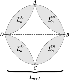
Figure 18: For $p=0$ or $p=1$, the lattice after $n+1$ construction steps, $L_{n+1}$, is composed of four copies of $L_{n}$ connected to one another as above. The $p=1$ case is shown above; for $p=0$ the horizontal long-range bond is absent.

A.2.1 Crossing paths $\Delta_{n}$ for $p=0$

Let $\Delta_{n}^{\alpha,\beta}$ denote the sum of all shortest paths with endpoints in $L_{n}^{(\alpha)}$ and $L_{n}^{(\beta)}$. If $L_{n}^{(\alpha)}$ and $L_{n}^{(\beta)}$ meet at an edge site, $\Delta_{n}^{\alpha,\beta}$ excludes paths where either endpoint is that shared edge site. If $L_{n}^{(\alpha)}$ and $L_{n}^{(\beta)}$ do not meet, $\Delta_{n}^{\alpha,\beta}$ excludes paths where either endpoint is any edge site. Then the total sum $\Delta_{n}$ is given by

$$\Delta_{n}= \,\Delta_{n}^{1,2}+\Delta_{n}^{2,3}+\Delta_{n}^{3,4}+\Delta_{n}^{4,1}+\Delta_{n}^{1,3}+\Delta_{n}^{2,4}$$

$$-2\cdot 2^{n+1}\,.$$ (85)

The last term at the end compensates for the overcounting of certain paths: the shortest path between $A$ and $C$, with length $2^{n+1}$, is included in both $\Delta_{n}^{2,3}$ and $\Delta_{n}^{4,1}$. Similarly the shortest path between $B$ and $D$, also with length $2^{n+1}$, is included in both $\Delta_{n}^{1,2}$ and $\Delta_{n}^{3,4}$.

By symmetry, $\Delta_{n}^{1,2}=\Delta_{n}^{2,3}=\Delta_{n}^{3,4}=\Delta_{n}^{4,1}$ and $\Delta_{n}^{1,3}=\Delta_{n}^{2,4}$, so that

$$\Delta_{n}=4\Delta_{n}^{1,2}+2\Delta_{n}^{1,3}-2\cdot 2^{n+1}\,.$$ (86)

$\Delta_{n}^{1,2}$ is given by the sum

$$\Delta_{n}^{1,2} =\sum_{\begin{subarray}{c}i\in L_{n}^{(1)},\,\,j\in L_{n}^{(2)}\\ i,j\neq A\end{subarray}}d_{ij}$$

$$=\sum_{\begin{subarray}{c}i\in L_{n}^{(1)},\,\,j\in L_{n}^{(2)}\\ i,j\neq A\end{subarray}}(d_{iA}+d_{Aj})$$

$$=(N_{n}-1)\sum_{i\in L_{n}^{(1)}}d_{iA}+(N_{n}-1)\sum_{j\in L_{n}^{(2)}}d_{Aj}$$

$$=2(N_{n}-1)\sum_{i\in L_{n}^{(1)}}d_{iA}\,,$$ (87)

where we have used $\sum_{i\in L_{n}^{(1)}}d_{iA}=\sum_{j\in L_{n}^{(2)}}d_{Aj}$. To find $\sum_{i\in L_{n}^{(1)}}d_{iA}$, we examine the structure of the hierarchical lattice at the $n$th level. $L_{n}^{(1)}$ contains $\nu_{n}(m)$ points with $d_{iA}=m$, where $1\leq m\leq 2^{n}$, and $\nu_{n}(m)$ can be written recursively as follows:

$$\nu_{n}(m)=\begin{cases}2^{n}&\text{if $m$ is odd}\,,\\ \nu_{n-1}(m/2)&\text{if $m$ is even}\,.\end{cases}$$ (88)

Expressing $\sum_{i\in L_{n}^{(1)}}d_{iA}$ in terms of $\nu_{n}(m)$,

$$f_{n}\equiv\sum_{i\in L_{n}^{(1)}}d_{iA}=\sum_{m=1}^{2^{n}}m\nu_{n}(m)\,.$$ (89)

Eqs. (88) and (89) relate $f_{n}$ and $f_{n-1}$, allowing the solution of $f_{n}$ by induction:

$$f_{n} =\sum_{k=1}^{2^{n-1}}(2k-1)2^{n}+\sum_{k=1}^{2^{n-1}}2k\nu_{n-1}(k)$$

$$=2^{3n-2}+2f_{n-1}$$

$$=\sum_{k=0}^{n-2}2^{k}2^{3(n-k)-2}+2^{n-1}f_{1}$$

$$=\frac{1}{3}2^{n}(2+4^{n})\,,$$ (90)

where we have used $f_{1}=\nu_{1}(1)+2\nu_{1}(2)=4$. Substituting Eq. (90) and $N_{n}=\frac{2}{3}(2+4^{n})$ into Eq. (87),

$$\Delta_{n}^{1,2}=\frac{1}{9}2^{1+n}(1+2^{1+2n})(2+4^{n})\,.$$ (91)

Proceeding similarly,

$$\Delta_{n}^{1,3}= \sum_{\begin{subarray}{c}i\in L_{n}^{(1)},\,\,j\in L_{n}^{(3)}\\ i\neq A,D,\,\,j\neq B,C\end{subarray}}d_{ij}$$

$$= \sum_{\begin{subarray}{c}i\in L_{n}^{(1)},\,\,j\in L_{n}^{(3)}\\ i\neq A,\,\,j\neq B,\,\,d_{iA}+d_{jB}<2^{n}\end{subarray}}(d_{iA}+2^{n}+d_{jB})$$

$$+\sum_{\begin{subarray}{c}i\in L_{n}^{(1)},\,\,j\in L_{n}^{(3)}\\ i\neq D,\,\,j\neq C,\,\,d_{iD}+d_{jC}<2^{n}\end{subarray}}(d_{iD}+2^{n}+d_{jC})$$

$$+\sum_{\begin{subarray}{c}i\in L_{n}^{(1)},\,\,j\in L_{n}^{(3)}\\ i\neq A,\,\,j\neq B,\,\,d_{iA}+d_{jB}=2^{n}\end{subarray}}2^{n+1}\,.$$ (92)

The first and second terms are equal and denoted by $g_{n}$, and the third term is denoted by $h_{n}$, so that $\Delta_{n}^{1,3}=2g_{n}+h_{n}$. The quantity $g_{n}$ is evaluated as follows:

$$g_{n}= \sum_{m=1}^{2^{n}-2}\>\sum_{m^{\prime}=1}^{2^{n}-1-m}\nu_{n}(m)\nu_{n}(m^{\prime})(m+2^{n}+m^{\prime})$$

$$= \sum_{k=1}^{2^{n-1}-2}\>\sum_{k^{\prime}=1}^{2^{n-1}-1-k}\nu_{n-1}(k)\nu_{n-1}(k^{\prime})(2k+2^{n}+2k^{\prime})$$

$$+\sum_{k=1}^{2^{n-1}-1}\>\sum_{k^{\prime}=1}^{2^{n-1}-k}\nu_{n-1}(k)2^{n}(2k+2^{n}+2k^{\prime}-1)$$

$$+\sum_{k=1}^{2^{n-1}-1}\>\sum_{k^{\prime}=1}^{2^{n-1}-k}2^{n}\nu_{n-1}(k^{\prime})(2k-1+2^{n}+2k^{\prime})$$

$$+\sum_{k=1}^{2^{n-1}-1}\>\sum_{k^{\prime}=1}^{2^{n-1}-k}2^{2n}(2k-1+2^{n}+2k^{\prime}-1)\,.$$ (93)

The fourth term can be summed directly, yielding

$$8^{n-1}(2^{n}-2)(5\cdot 2^{n}-2)/3\,.$$ (94)

The second and third terms in Eq. (93) are equal and can be simplified by first summing over $k^{\prime}$, yielding

$$2^{n-2}\sum_{k=1}^{2^{n-1}-1}\nu_{n-1}(k)(3\cdot 4^{n}-2^{n+2}k-4k^{2})\,.$$ (95)

For use in Eq. (95), $\sum_{k=1}^{2^{n-1}-1}\nu_{n-1}(k)=N_{n-1}-2$, and using Eq. (90),

$$\sum_{k=1}^{2^{n-1}-1}k\nu_{n-1}(k) =\sum_{k=1}^{2^{n-1}}k\nu_{n-1}(k)-2^{n-1}$$

$$=2^{n-1}(4^{n-1}-1)/3\,.$$ (96)

Analogously to Eq. (90), we find

$$\sum_{k=1}^{2^{n-1}-1}k^{2}\nu_{n-1}(k)=\frac{1}{9}2^{2n-3}(14+4^{n}-3n-3)-2^{n}\,.$$ (97)

With the latter results, Eq. (95) becomes

$$8^{n-1}(-23+5\cdot 4^{n}+3n)/9\,.$$ (98)

With Eqs. (94) and (98), Eq. (93) becomes

$$g_{n}=2g_{n-1}+8^{n-1}(-34-9\cdot 2^{n+2}+25\cdot 4^{n}+6n)/9\,.$$ (99)

Using $g_{1}=0$, Eq. (99) is solved inductively:

$$g_{n} =2^{n}(164-126\cdot 4^{n}-108\cdot 8^{n}+70\cdot 16^{n}$$

$$\qquad+21\cdot 4^{n}n)/189\,.$$ (100)

All that is left to find an expression for $\Delta_{n}^{1,3}$ is to evaluate

$$h_{n} =2^{n+1}\sum_{m=1}^{2^{n}-1}\nu_{n}(m)\nu_{n}(2^{n}-m)$$

$$=2^{n+1}\sum_{m=1}^{2^{n}-1}\nu^{2}_{n}(m)$$

$$=2^{n+1}\left[\sum_{k=1}^{2^{n-1}}4^{n}+\sum_{k=1}^{2^{n-1}-1}\nu^{2}_{n-1}(k)\right]$$

$$=16^{n}+2h_{n-1}\,,$$ (101)

where the symmetry $\nu_{n}(m)=\nu_{n}(2^{n}-m)$ was used. Using $h_{1}=16$, Eq. (101) is solved inductively:

$$h_{n}=2^{n+3}(8^{n}-1)/7\,.$$ (102)

From Eqs. (100) and (102),

$$\Delta_{n}^{1,3} =2^{n+1}(8-18\cdot 4^{n}+10\cdot 16^{n}+3\cdot 4^{n}n)/27\,.$$ (103)

Substituting Eqs. (91) and (103) into Eq. (86), we obtain the final expression for the crossing paths $\Delta_{n}$ when $p=0$:

$$\Delta_{n}=2^{2+n}(-7+3(4+n)4^{n}+22\cdot 16^{n})/27\,.$$ (104)

A.2.2 Crossing paths $\Delta_{n}$ for $p=1$

In the $p=1$ case, $\Delta_{n}$ is

$$\Delta_{n}^{1,2}+\Delta_{n}^{2,3}+\Delta_{n}^{3,4}+\Delta_{n}^{4,1}+\Delta_{n}^{1,3}+\Delta_{n}^{2,4}-3\,.$$ (105)

The last term compensates for the overcounting of the shortest path between $A$ and $C$, with length $2$, and the shortest path between $B$ and $D$, with length $1$.

Again by symmetry, $\Delta_{n}^{1,2}=\Delta_{n}^{3,4}$, $\Delta_{n}^{2,3}=\Delta_{n}^{4,1}$, and $\Delta_{n}^{1,3}=\Delta_{n}^{2,4}$, so that

$$\Delta_{n}=2\Delta_{n}^{1,2}+2\Delta_{n}^{2,3}+2\Delta_{n}^{1,3}-3\,.$$ (106)

We define

$$d_{n}^{\text{tot}} \equiv\sum_{i\in L_{n}^{(1)}}d_{iA}\,,$$

$$d_{n}^{\text{near}} \equiv\sum_{\begin{subarray}{c}i\in L_{n}^{(1)}\\ d_{iA}<d_{iD}\end{subarray}}d_{iA}\,,\qquad N_{n}^{\text{near}}\equiv\sum_{\begin{subarray}{c}i\in L_{n}^{(1)}\\ d_{iA}<d_{iD}\end{subarray}}1\,,$$

$$d_{n}^{\text{mid}} \equiv\sum_{\begin{subarray}{c}i\in L_{n}^{(1)}\\ d_{iA}=d_{iD}\end{subarray}}d_{iA}\,,\qquad N_{n}^{\text{mid}}\equiv\sum_{\begin{subarray}{c}i\in L_{n}^{(1)}\\ d_{iA}=d_{iD}\end{subarray}}1\,,$$

$$d_{n}^{\text{far}} \equiv\sum_{\begin{subarray}{c}i\in L_{n}^{(1)}\\ d_{iA}>d_{iD}\end{subarray}}d_{iA}\,,\qquad N_{n}^{\text{far}}\equiv\sum_{\begin{subarray}{c}i\in L_{n}^{(1)}\\ d_{iA}>d_{iD}\end{subarray}}1\,,$$ (107)

so that $d_{n}^{\text{tot}}=d_{n}^{\text{near}}+d_{n}^{\text{mid}}+d_{n}^{\text{far}}$ and $N_{n}=N_{n}^{\text{near}}+N_{n}^{\text{mid}}+N_{n}^{\text{far}}$. By symmetry $N_{n}^{\text{near}}=N_{n}^{\text{far}}$. Thus,

$$\Delta_{n}^{1,2} =\sum_{\begin{subarray}{c}i\in L_{n}^{(1)},\,\,j\in L_{n}^{(2)}\\ i,j\neq A\end{subarray}}d_{ij}=\sum_{\begin{subarray}{c}i\in L_{n}^{(1)},\,\,j\in L_{n}^{(2)}\\ i,j\neq A,\,\,d_{iA}\leq d_{iD}\end{subarray}}(d_{iA}+d_{Aj})$$

$$\quad+\sum_{\begin{subarray}{c}i\in L_{n}^{(1)},\,\,j\in L_{n}^{(2)},\,\,i,j\neq A\\ d_{iA}>d_{iD},\,\,d_{jA}\leq d_{jB}\end{subarray}}(d_{iA}+d_{Aj})$$

$$\quad+\sum_{\begin{subarray}{c}i\in L_{n}^{(1)},\,\,j\in L_{n}^{(2)},\,\,i,j\neq A\\ d_{iA}>d_{iD},\,\,d_{jA}>d_{jB}\end{subarray}}(d_{iD}+1+d_{Bj})$$

$$=\sum_{\begin{subarray}{c}i\in L_{n}^{(1)},\,\,i\neq A\\ d_{iA}\leq d_{iD}\end{subarray}}\left[(N_{n}-1)d_{iA}+d_{n}^{\text{tot}}\right]$$

$$\quad+\sum_{\begin{subarray}{c}i\in L_{n}^{(1)},\,\,i\neq A\\ d_{iA}>d_{iD}\end{subarray}}\left[(N_{n}^{\text{near}}+N_{n}^{\text{mid}}-1)d_{iA}+d_{n}^{\text{near}}+d_{n}^{\text{mid}}\right]$$

$$\quad+\sum_{\begin{subarray}{c}i\in L_{n}^{(1)},\,\,i\neq A\\ d_{iA}>d_{iD}\end{subarray}}\left[N_{n}^{\text{near}}(d_{iD}+1)+d_{n}^{\text{near}}\right]$$

$$=(N_{n}-1)(d_{n}^{\text{near}}+d_{n}^{\text{mid}})+(N_{n}^{\text{near}}+N_{n}^{\text{mid}}-1)d_{n}^{\text{tot}}$$

$$\quad+(N_{n}^{\text{near}}+N_{n}^{\text{mid}}-1)d_{n}^{\text{far}}+N_{n}^{\text{near}}(d_{n}^{\text{near}}+d_{n}^{\text{mid}})$$

$$\quad+N_{n}^{\text{near}}(d_{n}^{\text{near}}+N_{n}^{\text{near}})+N_{n}^{\text{near}}d_{n}^{\text{near}}\,.$$ (108)

The horizontal long-range bond does not affect $\Delta_{n}^{2,3}$, so that Eq. (87) still holds, $\Delta_{n}^{2,3}=2(N_{n}-1)d_{n}^{\text{tot}}$. Finally,

$$\Delta_{n}^{1,3} =\sum_{\begin{subarray}{c}i\in L_{n}^{(1)},\,\,j\in L_{n}^{(3)}\\ i\neq A,D,\,\,j\neq B,C\end{subarray}}d_{ij}=\sum_{\begin{subarray}{c}i\in L_{n}^{(1)},\,\,j\in L_{n}^{(3)}\\ i\neq A,D,\,\,j\neq B,C,\,\,d_{jB}>d_{jC}\end{subarray}}(d_{iD}+1+d_{Cj})$$

$$\quad+\sum_{\begin{subarray}{c}i\in L_{n}^{(1)},\,\,j\in L_{n}^{(3)},\,\,i\neq A,D\\ j\neq B,C,\,\,d_{iA}\geq d_{iD},\,\,d_{jB}\leq d_{jC}\end{subarray}}(d_{iD}+1+d_{Bj})$$

$$\quad+\sum_{\begin{subarray}{c}i\in L_{n}^{(1)},\,\,j\in L_{n}^{(3)},\,\,i\neq A,D\\ j\neq B,C,\,\,d_{iA}<d_{iD},\,\,d_{jB}\leq d_{jC}\end{subarray}}(d_{iA}+1+d_{Bj})$$

$$=\sum_{i\in L_{n}^{(1)},\,\,i\neq A,D}\left[(N_{n}^{\text{near}}-1)(d_{iD}+1)+d_{n}^{\text{near}}\right]$$

$$\quad+\sum_{\begin{subarray}{c}i\in L_{n}^{(1)},\,\,i\neq A,D\\ d_{iA}\geq d_{iD}\end{subarray}}\left[(N_{n}^{\text{near}}+N_{n}^{\text{mid}}-1)(d_{iD}+1)\right.$$

$$\quad\qquad\qquad\left.+d_{n}^{\text{near}}+d_{n}^{\text{mid}}\right]$$

$$\quad+\sum_{\begin{subarray}{c}i\in L_{n}^{(1)},\,\,i\neq A,D\\ d_{iA}<d_{iD}\end{subarray}}\left[(N_{n}^{\text{near}}+N_{n}^{\text{mid}}-1)(d_{iA}+1)\right.$$

$$\quad\qquad\qquad\left.+d_{n}^{\text{near}}+d_{n}^{\text{mid}}\right]$$

$$=(N_{n}^{\text{near}}-1)(d_{n}^{\text{tot}}-1+N_{n}-2)+(N_{n}-2)d_{n}^{\text{near}}$$

$$\quad+(N_{n}^{\text{near}}+N_{n}^{\text{mid}}-1)(d_{n}^{\text{near}}+d_{n}^{\text{mid}}+N_{n}^{\text{near}}+N_{n}^{\text{mid}}-1)$$

$$\quad\qquad\qquad+(N_{n}^{\text{near}}+N_{n}^{\text{mid}}-1)(d_{n}^{\text{near}}+d_{n}^{\text{mid}})$$

$$\quad+(N_{n}^{\text{near}}+N_{n}^{\text{mid}}-1)(d_{n}^{\text{near}}+N_{n}^{\text{near}}-1)$$

$$\quad\qquad\qquad+(N_{n}^{\text{near}}-1)(d_{n}^{\text{near}}+d_{n}^{\text{mid}})\,.$$ (109)

Having $\Delta_{n}^{1,2}$, $\Delta_{n}^{2,3}$, and $\Delta_{n}^{1,3}$ in terms of the quantities in Eq. (107), the next step is to explicitly determine these quantities.

Figure 19: The first three construction steps of the lattice with $p=1$, with the sites labeled by ordered pairs denoting the shortest-path distance to the left and right edge sites.

We consider a site $i\in L_{n}^{(1)}$ and the shortest-path distances to the edges, $d_{iA}$ and $d_{iD}$. If the site was added to the lattice at the $n$th construction step, the values of $d_{iA}$ and $d_{iD}$ do not change at subsequent steps, since the shortest path to the edge sites is always along the bonds added earliest. We see this in Fig. 19, where the sites are labeled by the ordered pairs $d_{iD},\,d_{iA}$, for the first three construction steps. We denote by $a^{n}_{m,m^{\prime}}$ the number of sites added at the $n$th construction step which have $d_{iA}=m$, $d_{iD}=m^{\prime}$. Since $A$ and $D$ are connected by a long-range bond, $m^{\prime}$ and $m$ can differ by at most 1. Thus for a given $m$ there are three categories of sites added at step $n$, respectively numbering $a^{n}_{m,m+1},a^{n}_{m,m}$, and $a^{n}_{m+1,m}$. By symmetry $a^{n}_{m+1,m}=a^{n}_{m,m+1}$. The $m$, $m^{\prime}$ values of sites added at step $n$ depend on the neighboring sites, which were added at previous construction steps. For example, there are $2^{n}$ sites added at the $n$th step ($n\geq 2$) which are nearest-neighbors of site $A$, so these new sites have $m=1$, $m^{\prime}=2$, giving $a^{n}_{1,2}=2^{n}$. Sites with $m=1$, $m^{\prime}=2$ will in turn get neighbors with $m=2$, $m^{\prime}=3$ in subsequent steps. The relationship between $a^{n}_{2,3}$ and $a^{k}_{1,2}$ for $k<n$ is

$$a^{n}_{2,3}=\sum_{k=2}^{n-2}2^{n+1-k}a^{k}_{1,2}=2^{n+1}(n-3)\,.$$ (110)

Similarly,

$$a^{n}_{3,4}=\sum_{k=4}^{n-2}2^{n+1-k}a^{k}_{2,3}=2^{n+1}(n-4)(n-5)\,.$$ (111)

Since sites with distances $m$, $m+1$ do not appear before the construction step $n=2m$, the sum over $a^{k}_{2,3}$ starts at $k=4$. Proceeding in this manner, for general $m\geq 1$ and $n\geq 2m$,

$$a^{n}_{m,m+1} =\sum_{k=2(m-1)}^{n-2}2^{n+1-k}a^{k}_{m-1,m}$$

$$=\frac{2^{m-1}2^{n}(n-m-1)!}{(m-1)!(n-2m)!}\,.$$ (112)

The value of $a^{n}_{0,1}$ is $1$ for $n=0$ and $0$ for $n>0$. Analogously, for general $m\geq 2$ and $n\geq 2m-1$,

$$a^{n}_{m,m}=\frac{2^{m-1}2^{n}(n-m-1)!}{(m-2)!(n-2m+1)!}\,.$$ (113)

The value of $a^{n}_{1,1}$ is $2$ for $n=1$ and $0$ for $n>1$.

Thus we obtain the quantities in Eq. (107),

$$N^{\text{near}}_{n} =\sum_{n^{\prime}=1}^{n}\sum_{k=1}^{\lfloor n^{\prime}/2\rfloor}a^{k}_{m,m+1}=\begin{cases}1+\frac{2}{9}(2^{n}+4^{n}-2)\\ 1+\frac{2}{9}(2^{n}-2)(2^{n}+1)\end{cases}$$

$$N^{\text{mid}}_{n} =\sum_{n^{\prime}=1}^{n}\sum_{k=1}^{\lfloor(n^{\prime}+1)/2\rfloor}a^{k}_{m,m}=\begin{cases}\frac{2}{9}(2^{n}-1)^{2}\\ \frac{2}{9}(2^{n}+1)^{2}\end{cases}$$

$$d^{\text{near}}_{n} =\sum_{n^{\prime}=1}^{n}\sum_{k=1}^{\lfloor n^{\prime}/2\rfloor}ma^{k}_{m,m+1}=\begin{cases}\frac{2}{81}(2^{n}+2)(2^{n}+3\cdot 2^{n}n-1)\\ \frac{2}{81}(2^{n}-2)(2^{n}+3\cdot 2^{n}n+1)\end{cases}$$

$$d^{\text{mid}}_{n} =\sum_{n^{\prime}=1}^{n}\sum_{k=1}^{\lfloor(n^{\prime}+1)/2\rfloor}ma^{k}_{m,m}$$

$$=\begin{cases}\frac{2}{81}\left[-2^{n+3}-12\cdot 2^{n}n+(3n+7)4^{n}+1\right]\\ \frac{2}{81}\left[2^{n+3}+7\cdot 4^{n}+3n(2^{2+n}+4^{n})+1\right]\end{cases}$$

where $\lfloor x\rfloor$ denotes the largest integer $\leq x$ and the different results for $n$ even and odd are given consecutively, and

$$d^{\text{far}}_{n} =\sum_{n^{\prime}=1}^{n}\sum_{k=1}^{\lfloor n^{\prime}/2\rfloor}(m+1)a^{k}_{m,m+1}=d_{n}^{\text{near}}+N_{n}^{\text{near}}\,.$$ (115)

Substituting the results of Eq. (LABEL:eq:app40) into Eqs. (108)-(109), for $p=1$,

$$\Delta_{n} =\frac{1}{27}\left[-23-8(-2)^{n}+8\cdot 4^{n}+(104+48n)16^{n}\right].$$ (116)

Substituting Eqs. (104) and (116) for $\Delta_{m}$ into Eq. (84), and using $S_{1}=8,7$ for $p=0,1$,

$$S_{n}=\begin{cases}\frac{2^{n}}{189}\left[98+27\cdot 2^{n}+(42+21n)4^{n}+22\cdot 16^{n}\right]\\ \frac{1}{81}\left[23+4(-2)^{n}+(44+6n)4^{n}+(10+12n)16^{n}\right]\end{cases}$$ (117)

Eq. (117) in Eq. (81) yields the analytical expressions for $\ell_{n}$ in Eqs. (II.2.3) and (II.2.3).

References

- (1) R. Albert and A.-L. Barabási, Rev. Mod. Phys. 74, 47 (2002).
- (2) M.E.J. Newman, SIAM Review 45, 167 (2003).
- (3) S.N. Dorogovtsev and J.F.F. Mendes, Adv. Phys. 51, 1079 (2002).
- (4) D.J. Watts and S.H. Strogatz, Nature 393, 440 (1998).
- (5) A.L. Barabási and R. Albert, Science 286, 509 (1999).
- (6) M. Gitterman, J. Phys. A: Math. Gen. 33, 8373 (2000).
- (7) A. Barrat and M. Weigt, Eur. Phys. J. B 13, 547 (2000).
- (8) A. Pȩkalski, Phys. Rev. E 64, 057104 (2001).
- (9) H. Hong, B.J. Kim, and M.Y. Choi, Phys. Rev. E 66, 018101 (2002).
- (10) D. Jeong, H. Hong, B.J. Kim, and M.Y. Choi, Phys. Rev. E 68, 027101 (2003).
- (11) B.J. Kim, H. Hong, P. Holme, G.S. Jeon, P. Minnhagen, and M.Y. Choi, Phys. Rev. E 64, 056135 (2001).
- (12) A. Aleksiejuk, J.A. Holyst, and D. Stauffer, Physica A 310, 260 (2002).
- (13) G. Bianconi, Phys. Lett. A 303, 166 (2002).
- (14) S.N. Dorogovtsev, A.V. Goltsev, and J.F.F. Mendes, Phys. Rev. E 66, 016104 (2002).
- (15) M. Leone, A. Vázquez, A. Vespignani, and R. Zecchina, Eur. Phys. J. B 28, 191 (2002).
- (16) A.V. Goltsev, S.N. Dorogovtsev, and J.F.F. Mendes, Phys. Rev. E 67, 026123 (2003).
- (17) A.N. Berker and S. Ostlund, J. Phys. C 12, 4961 (1979).
- (18) M. Kaufman and R.B. Griffiths, Phys. Rev. B 24, 496 (1981).
- (19) M. Kaufman and R.B. Griffiths, Phys. Rev. B 30, 244 (1984).
- (20) A.-L. Barabási, E. Ravasz, and T. Vicsek, Physica A 299 (2001).
- (21) S.N. Dorogovtsev, J.F.F. Mendes, and A.N. Samukhin Phys. Rev. E 63, 062101 (2001).
- (22) S.N. Dorogovtsev, A.V. Goltsev, and J.F.F. Mendes, Phys. Rev. E 65, 066122 (2002).
- (23) F. Comellas and M. Sampels, Physica A 309, 231 (2002).
- (24) S. Jung, S. Kim, and B. Kahng, Phys. Rev. E 65, 056101 (2002).
- (25) Z. Zhang, L. Rong, and C. Guo, cond-mat/0502335.
- (26) J.S. Andrade Jr., H.J. Herrmann, R.F.S. Andrade, and L.R. Silva, Phys. Rev. Lett. 94, 018702 (2005).
- (27) T. Zhou, G. Yan, and B.-H. Wang, Phys. Rev. E 71, 046141 (2005).
- (28) R.F.S. Andrade and H.J. Herrmann, Phys. Rev. E 71, 056131 (2005).
- (29) V.L. Berezinskii, Sov. Phys. JETP 32, 493 (1971).
- (30) J.M. Kosterlitz and D.J. Thouless, J. Phys. C 6, 1181 (1973).
- (31) D.S. Callaway, J.E. Hopcroft, J.M. Kleinberg, M.E.J. Newman, and S.H. Strogatz, Phys. Rev. E 64, 041902 (2001).
- (32) S.N. Dorogovtsev, J.F.F. Mendes, and A.N. Samukhin, Phys. Rev. E 64, 066110 (2001).
- (33) J. Kim, P.L. Krapivsky, B. Kahng, and S. Redner, Phys. Rev. E 66, 055101 (2002).
- (34) D. Lancaster, J. Phys. A 35, 1179 (2002).
- (35) M. Bauer and D. Bernard, J. Stat. Phys. 111, 703 (2003).
- (36) S. Coulomb and M. Bauer, Eur. Phys. J. B 35, 377 (2003).
- (37) B. Bollobás, S. Janson, and O. Riordan, Random Struct. Algorithms 26, 1 (2005).
- (38) P.L. Krapivsky and B. Derrida, Physica A 340, 714 (2004).
- (39) M. Bauer, S. Coulomb, and S.N. Dorogovtsev, Phys. Rev. Lett. 94, 200602 (2005).
- (40) O. Costin, R.D. Costin, and C.P. Grunfeld, J. Stat. Phys. 59, 1531 (1990).
- (41) O. Costin and R.D. Costin, J. Stat. Phys. 64, 193 (1991).
- (42) M. Bundaru and C.P. Grunfeld, J. Phys. A 32, 875 (1999).
- (43) S. Romano, Mod. Phys. Lett. B 9, 1447 (1995).
- (44) A.A. Migdal, Zh. Eksp. Teor. Fiz. 69, 1457 (1975) [Sov. Phys. JETP 42, 743 (1976)].
- (45) L.P. Kadanoff, Ann. Phys. (N.Y.) 100, 359 (1976).
- (46) S.R. McKay and A.N. Berker, Phys. Rev. B 29, 1315 (1984).
- (47) A.N. Berker, S. Ostlund, and F.A. Putnam, Phys. Rev. B 17, 3650 (1978).
- (48) A.N. Berker and D.R. Nelson, Phys. Rev. B 19, 2488 (1979).
- (49) D. Andelman and A.N. Berker, Phys. Rev. B 29, 2630 (1984).
- (50) A. Falicov, A.N. Berker, and S.R. McKay, Phys. Rev. B 51, 8266 (1995).
- (51) J. Candia, cond-mat/0602192.