Self-Organized Dynamical Equilibrium in the Corrosion of Random Solids

Abstract

Self-organized criticality is characterized by power law correlations in the non-equilibrium steady state of externally driven systems. A dynamical system proposed here self-organizes itself to a critical state with no characteristic size at “dynamical equilibrium”. The system is a random solid in contact with an aqueous solution and the dynamics is the chemical reaction of corrosion or dissolution of the solid in the solution. The initial difference in chemical potential at the solid-liquid interface provides the driving force. During time evolution, the system undergoes two transitions, roughening and anti-percolation. Finally, the system evolves to a dynamical equilibrium state characterized by constant chemical potential and average cluster size. The cluster size distribution exhibits power law at the final equilibrium state.

The phenomenon that a class of externally driven system evolves naturally into a state of no single characteristic size or time is known as self-organized criticality (SOC)jensen . SOC is observed in several situations like sandpilebak , earthquakesearthq , forest fireff , coagulationcoag , river networksrnetw , etc. The models demonstrating SOC are in out of equilibrium situations. The non-equilibrium steady state in SOC is characterized by long range spatio-temporal correlations and power law scaling behaviour.

In this paper, a system is demonstrated which is evolving naturally into a dynamical equilibrium state with no characteristic size. The system considered here is the corrosion or dissolution of a random solid in an aqueous solution. The initial difference in the chemical potential of the solid-liquid interface drives the system and no other external force is applied. A random solid could be a multicomponent vitreous system in which, due to random local chemical environment, the binding energies of the constituent molecules of the solid are expected to be arbitrary. In order to study the time evolution of such a system in aqueous solution, a numerical model of corrosion or dissolution is developed in $2$ dimensions ($2D$). In this model, it is assumed that the random binding energy is uniformly distributed between $0$ and $1$. The solid shown in figure 1 ($a$) is a dense structure of elements with random binding energy $r_{i}$. The solid is placed in an aqueous solution, assumed to be infinite. The white space in figure 1 represents the solution. Random solid element $R$ dissolves slowly in the solution $S$, makes a compound $RS$ and the compound breaks instantaneously into $R$ and $S$. The chemical reaction of dissolution could be represented as

$$R+S\rightarrow RS\rightarrow R+S.$$ (1)

The solid element $R$ in the solution is now available for redeposition on the interface. Assuming diffusion of the solid element $R$ is very fast in the solution, redeposition is made at a randomly chosen site on the externally accessible perimeter with unit probability. Generally, dissolution is a slow process and redeposition is faster. It is mimicked here by considering no further dissolution during redeposition. The slowest possible dynamics of the system then involves dissolution and redeposition processes together with reconstruction of the rough interface at the single particle level. Different numerical processes involved in a single Monte Carlo (MC) step are explained with the help of figure 1. The process are: $(i)$ extraction of externally accessible perimeter of the solid, $(ii)$ dissolution of the site with minimum random number (minimum binding energy) on the perimeter with unit probability (in figure 1 ($b$), it is $r_{14}$), $(iii)$ modification of the external perimeter, $(iv)$ redeposition of the solid element present in the solution on a randomly chosen site of the modified external perimeter ($r_{3}$ in figure 1 $(c)$), $(v)$ assignment of a new random number $r_{\alpha}$ to the redeposited site. The whole process is then repeated and time is increased from $t$ to $t+1$. Note that the total number of particles $(L^{2})$ is conserved and the system evolves at equal solid to liquid and liquid to solid flux rate (one particle per time step) throughout the simulation.

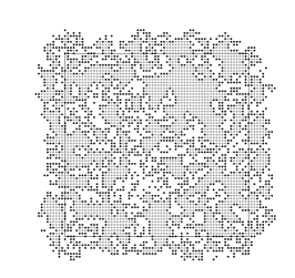
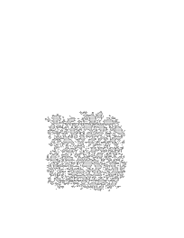
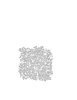
$(a)$ $t=2^{13}$ $(b)$ $t=2^{20}$ $(c)$ $t=2^{24}$

Figure 2: Morphology of the random solid system at three different times. Black dots are the externally accessible perimeter sites in contact with the solution. Gray dots are the interior solid sites, not in contact with the solution at that time. White space represents the solution. The solid line represents the lattice boundary at $t=0$.

Simulations have been performed on the square lattice of sizes ranging from $L=8$ to $L=128$. Data are averaged over $\mathcal{N}_{S}=1000$ to $10000$ samples. In figure 2, time evolution of the system morphology is shown for a system of size $L=64$ at three different times $t=2^{12}$ $(a)$, $2^{20}$ $(b)$, and $2^{24}$ $(c)$. It can be seen that the system first becomes rough or porous, then the infinite network of solid elements breaks into small finite clusters (anti-percolation or dissolution) and finally equilibrates to a morphology which remains almost unaltered over a long period of time. A cluster of size $s$ contains $s$ number of atoms or molecules connected by nearest neighbour bonds. The time evolution of the system then has three different regimes, initial - porous, intermediate - dissolution and final - dynamical equilibrium. There is also slow dispersion of the clusters radially outward. It should be mentioned here that in the study of self-stabilized etching of random solids by finite etching solution (infinite solid and finite solution)epl_physa final stable morphology obtained was fractal as it was observed by Balázs in the corrosion of thin metal filmsbalazs . In the following, different transitions will be identified and the final equilibrium state of the system will be characterized.

To determine the roughening or porosity transition, number of externally accessible perimeter (hull) sites $h$ is counted with time. The externally accessible perimeter sites, defined by Grossman and Aharonygross , include the sites available to the solution molecules, touching the occupied sites of the clusters available at that time. There are some standard methods for determining the external perimeter or cluster hull like Ziff walk, kinetic walkziff etc. However, instead of performing some walks around the individual clusters, the time evolution of the hull itself could be followed. At $t=0$, a string of lattice site index of all the boundary sites is considered. The site with minimum random number is taken out of the string and the string is locally modified depending on the local environment in the original lattice. A string index is then randomly chosen. A new random number is included at that position and the string is locally modified again according to the local environment in the original lattice. The hull string is then updated at each time step. The total number of particles stored in this string is the measure of the hull size. Note that, the string could be a collection of hulls of all disconnected finite clusters and may not represent a continuous path of perimeter sites of a single cluster. In figure 3($a$), normalized perimeter size $H=h/4L$ is plotted against $t$. Initially $H$ increases slowly with time and finally saturates followed by a rapid change in between. The roughening transition corresponds to the maximum time rate of change of $H$. The logarithmic time derivatives $dH/Dt$ ($Dt=d\log_{2}t$) are plotted in figure 3($b$) against $t$. It could be checked that the maxima of $dH/Dt$ correspond to the highly porous morphology of the system in figure 2 at $t=2^{13}$ for $L=64$. Notice that the infinite network of solid elements still exists at this time. As the roughening time $t_{r}$ is lattice size dependent, a scaling relation for $t_{r}$ with $L$ is proposed as $t_{r}=2^{-5}\times L^{3}$. Note that, $t_{r}$ increse as $L^{3}$ and not as $L^{2}$, total number of particles. The derivatives $dH/Dt$ are now plotted against the scaled roughening time $t_{r}^{\prime}=t_{r}/(2^{-5}\times L^{3})$ in the inset of figure 3($b$). Though there is not a good collapse of data for $t_{r}^{\prime}<1$ but it is clear that the transition occurs around $t_{r}^{\prime}=1$ independent of system size. It is important now to consider the time evolution of the random numbers $r_{h}$ of the solid elements on the hull. In figure 3($c$), $\langle r_{h}\rangle=\sum_{i}^{h}r_{i}/h$ is plotted against $t$. As the system evolves, $\langle r_{h}\rangle$ increases and saturates to unity. However, the dynamics of dissolution and redeposition will continue with the prefixed flux rate since by definition a site with lowest random number will always dissolve. The dynamics is not only independent of the absolute value of $r_{i}$ but also independent of its distribution. For example, random solid with random numbers uniformly distributed between $0.5$ to $1$ will not have different dynamics. It is interesting to notice that the evolution of $\langle r_{h}\rangle$ has a plateau just before the roughening transition and then it evolves again to another state of constant $\langle r_{h}\rangle$. Before the roughening transition the evolution then slows down temporarily and evolves again with higher speed to another steady state. The plateau in $\langle r_{h}\rangle$ could represent a “pseudo equilibrium” corresponding to a transient state. Appearance of pseudo equilibrium was also observed in the dissolution study of multicomponent random solidsantra .

The present model of interface evolution has great similarity with the Bak-Snappen (BS) model of biological evolutionbs . In the BS model, time evolution of the fitness string of a number of species was considered. The fitness of a species was represented by a random number uniformly distributed between $0$ and $1$. The species with lowest fitness (lowest random number) was replaced by another random number and the fitness string was locally modified as the hull is modified locally here in the present problem. The BS model self-organizes into a critical state with intermittent co-evolutionary avalanches of all sizes representing punctuated equilibrium behaviour of the evolution process. The average random number of the hull equivalent to the global fitness shows only one plateau during the time evolution of the interface. The fitness string in the BS model never had a hole, always a single continuous string, unlike the hull here which could be a collection of external perimeters of all finite disconnected clusters.

Far from the roughening transition, the dissolution or anti-percolation transition occurs in the system when $\langle r_{h}\rangle$ saturates to unity. At the anti-percolation transition, the infinite network of the random solid breaks into small finite clusters for the first time. The probability to have an $s$-sited cluster at time $t$ is given by

$$P_{s}(t)=n_{s}(t)/N_{tot}(t)$$ (2)

where $n_{s}(t)$ is the number of $s$-sited cluster out of total $N_{tot}$ clusters at that time. To identify the anti-percolation transition, average cluster size $\chi(t)=\sum s^{2}P_{s}(t)/\sum sP_{s}(t)$ is calculated as function of time. Note that the sum is over all possible clusters including the largest cluster, unlike percolationperco . $\chi(t)$ is plotted against $t$ in figure 4($a$). It can be seen that the average cluster size remains almost constant initially then decreases rapidly during the anti-percolation transition and finally saturates to a small value. Dissolution time $t_{d}$ is determined from the maximum time rate of change of $\chi(t)$. The logarithmic time derivative $d\chi/Dt$ of the average cluster size is plotted against $t$ in figure 4($b$). The dips in the plots correspond to the anti-percolation or dissolution at which the infinite network disappears from the system for the first time. The corresponding morphology is shown in figure 2($b$) at $t=2^{20}$ for $L=64$. A scaling form $t_{d}=L^{2}\times 2^{L/8}$ is suggested for $L$ dependent dissolution time. $d\chi/Dt$ is now plotted against the scaled dissolution time $t_{d}^{\prime}=t_{d}/(L^{2}\times 2^{L/8})$ in the inset of figure 4($b$). A reasonable data collapse is observed. The system then undergoes an anti-percolation transition at $t_{d}^{\prime}=1$ independent of system size. The dissolution time $t_{d}$ can also be estimated from the total number of clusters $N_{tot}(t)$ generated with time. The time rate of change of $N_{tot}$, $dN_{tot}/Dt$, is plotted in figure 4($c$) for different lattice sizes. The maximum cluster generation occurs at $t=t_{d}$ and then the rate of cluster generation decreases. Notice that roughening time $t_{r}$ and dissolution time $t_{d}$ scales very differently, $t_{r}$ increases as $L^{3}$ whereas $t_{d}$ increases exponentially with $L$.

The system is then allowed to evolve further, far from the anti-percolation transition. As $t\rightarrow\infty$, it is already seen that hull size $h$ and average cluster size $\chi$ are going to saturate to some finite values. Now it is important to consider the evolution of all the random numbers instead that of only the hull. Average random number $\langle r\rangle=\sum_{i}^{L^{2}}r_{i}/L^{2}$ of all the sites and $d\langle r\rangle/Dt$ are plotted against $t$ in figure 5($a$) for $L=32$ starting from porosity transition $t_{r}=2^{10}$. Notice that $\langle r\rangle$ saturates to one just after the anti-percolation transition and $d\langle r\rangle/Dt$ goes to zero. Since $\langle r\rangle$ is close to one, it is expected that most of the particles have changed their random numbers or dissolved at least once. The probability $P_{e}(t)$ to have a sample at time $t$ with all the sites dissolved at least once is calculated. It is defined as $P_{e}(t)=\mathcal{N}_{d}(t)/\mathcal{N}_{S}$ where $\mathcal{N}_{d}(t)$ is the number of samples for which all the sites dissolved at least once by time $t$ out of $\mathcal{N}_{S}$ samples. It is plotted in figure 5($b$) against $t$ for $L=16$ and $32$. A time $t_{e}$ is defined corresponding to the maximum change in $P_{e}$ at which all the sites of $50\%$ samples dissolved at least once. It is obtained as $t_{e}=2^{14}$ for $L=8$, $t_{e}=2^{16}$ for $L=16$, $t_{e}=2^{19}$ for $L=32$ and $t_{e}=2^{24}$ for $L=64$. It is interesting to notice that the logaritghmic difference in $t_{e}$ and $t_{d}$ is decreasing with the system size. $\log_{2}(t_{e}/t_{d})$ is plotted in the inset of ($b$) with $\log_{2}L$. The difference vanishes at $L=2^{10}$. Thus, beyond the system size of $2^{10}$ all the sites will dissolve at least once by the dissolution time $t_{d}$. The situation can be called as complete dissolution. At this stage, the small finite clusters in the solution can be considered as a single fluidized particle phase of the system and the dynamics is fragmentation of a particle in one cluster and coagulation at another cluster with a slow radially outward dispersion of the clusters. Constant average cluster size $\chi$ suggests that the cluster size distribution remains invariant over time at this phase. It is verified by plotting the cluster size distribution $P_{s}(t)$ at $t\geq t_{e}$ for different $L$ in figure 5($c$). The distributions collapse onto a single curve for different $t$ and $L$. Note that for $L=16$, the distribution remains invariant for $t=2^{16}(t_{e})$ to $t=2^{24}$. The distribution follows a power law with an exponent $\tau^{\prime}\approx 1.67$. The same slope is also obtained for $P_{s}=n_{s}/L^{2}$ distribution, as in percolation, since after dissolution time $t_{d}$ there will be very few cluster generation for large systems. It is then a critical state of the system with no characteristic size. After anti-percolation, the system then sattels into a state of constant cluster size distribution through critical slowing down ($d\langle r\rangle/Dt=0$). The final fluidized particle phase of the system then can be considered as a dynamical equilibrium state characterized by constant chemical potential (saturated hull size) and constant average cluster size. The transitions observed here during time evolution are features of slow dynamics considered in the system. Inclusion of rapid dynamics in the system could musk all these transitions and the system may evolve directly to the final equilibrium state.

The anti-percolation transition discussed above is very similar to fragmentation phenomena in $2D$. In the case of fragmentation, the system equilibrates after complete dissipation of the impact force and a power law distribution of the fragment mass ($m$) was obtained $i.e.$; $n(m)\sim m^{-\tau}$. The critical behaviour of fragmentation was studied by Kun and Herrmannhans and found that it belongs to the same universality class of percolation, $i.e.$; $\tau=187/91$perco . However, in a recent experiment of fragmentation of brittle solids by Katsuragi et alkatsu it is found that $\tau\approx 1.5$, different from percolation. The exponent obtained here ($1.67$) for the cluster size distribution at the anti-percolation transition is different from both Katsuragi exponent in the case of fragmentation as well as that of percolation.

In conclusion, the chemical reaction of dissolution of a random solid in a solution is modeled. The model demonstrates different transitions like roughening or porosity, dissolution or anti-percolation during time evolution. The transitions physically correspond to the maximum solid-liquid interface and disappearance of the infinite cluster respectively. Different transition times are found scaling very differently with the system size. Finally the system evolves to a dynamical equilibrium state through critical slowing down charcterized by constant cluster size distribution. The dynamical system considered here, driven by the initial difference in chemical potential, self-organizes itself into a critical state with no characteristic size at dynamical equilibrium. This is a new phenomenon. Generally, the dynamical systems, driven externally, self-organizes themselves to a non-equilibrium steady state characterized by power law correlations as observed in SOC models. The phenomena observed here should exists in $3D$ systems. The present model has relevance with other widely different models like biological evolution or fragmentation of brittle solids. The model could also be useful in understanding time evolution of waste disposal glasses.

The authors thank B. Sapoval, I. Bose and A. Srinivasan for critical comments. SS thanks CSIR, India for financial support.

$(a)$ $(b)$ $(c)$

Figure 1: A single Monte Carlo (MC) step is represented here. $(a)$ The arrangement of random numbers $r_{i}$ represents a random solid, $(b)$ $r_{14}$ is identified as minimum random number on the external boundary of the solid and it is dissolved, $(c)$ the solid element is redeposited at a randomly chosen site $r_{3}$ of the modified solid surface. A new random number $r_{\alpha}$ is associated with the redeposited site. The process is repeated.

Figure 3: $(a)$ Normalized hull size $H=h/4L$ and $(b)$ its logarithmic time derivatives $dH/Dt$ ($Dt=d\log_{2}t$) are plotted against time $t$. The symbols are: circles for $L=8$, squares for $L=16$, diamonds for $L=32$, triangles for $L=64$ and crosses for $L=128$. In the inset of ($b$), $dH/Dt$ is plotted against scaled roughening time $t_{r}^{\prime}$. The height of the plots are adjusted to unity. Data for all the systems collapse reasonably around $t_{r}^{\prime}=1$. $(c)$ Plot of $\langle r_{h}\rangle$, average random numbers of the interface, against $t$.

Figure 4: Plot of (a) average cluster size $\chi(t)$, (b) its logarithmic time derivative $d\chi/Dt$ ($Dt=d\log_{2}t$) against $t$. $\chi$ is normalized to unity dividing by the total number of particles $L^{2}$. In the inset of ($b$), $d\chi/Dt$ is plotted against scaled dissolution time $t^{\prime}_{d}$. The height of the plots are normalized to unity. ($c$) Plot of $dN_{tot}/Dt$ against $t_{d}^{\prime}$ indicates maximum cluster generation at $t_{d}^{\prime}=1$. The same symbol set for different $L$ of the previous figure is used. For $L=128$, dissolution does not occur by $t=2^{24}$ time steps.

Figure 5: ($a$) Plot of $\langle r\rangle$ ($\diamondsuit$) and $d\langle r\rangle/Dt$ ($+$) against $t$ for $L=32$. Arrows indicate dissolution time. ($b$) Plot of $P_{e}(t)$ for $L=16$ ($\Box$) and $32$ ($\diamondsuit$). In the inset, scaling of $t_{e}/t_{d}$ with $L$ is shown. Difference between $t_{d}$ and $t_{e}$ vanishes at $L=2^{10}$. ($c$) Plot of cluster size distributions $P_{s}(t)$ at different times for $t\geq t_{e}$ for different lattice sizes. Symbols are explained in the legend. The straight line with slope $\approx 1.67$ is guide to eye.

References

- (1) H. J. Jensen, Self-Organized Criticality, (Cambridge, 1998).
- (2) P. Bak, C. Tang and K. Wiesenfeld, Phys. Rev. Lett. 59, 381 (1987); Phys. Rev. A 38, 364 (1988).
- (3) K. Chen, P. Bak and S. P. Obukhov, Phys. Rev A 43, 625 (1990); K. Ito, Phys. Rev. E 52, 3232 (1995).
- (4) M. Paczuski and P. Bak, Phys. Rev. E 48 R3214 (1993); B. Drossel, S. Clar and F. Schwabl, Phys. Rev. Lett. 71, 3739 (1993).
- (5) H. Takayasu, Phys. Rev. Lett. 63, 2563 (1989); J. Ke and Z. Lin, Phys. Rev. E 66, 062101 (2002).
- (6) H. Takayasu and H. Inaoka, Phys. Rev. Lett. 68, 966 (1992); A. Rinaldo et al, Phys. Rev. Lett. 70, 822 (1993).
- (7) B. Sapoval, S. B. Santra and Ph. Barboux, Europhys. Lett. 41, 297 (1998); S. B. Santra and B. Sapoval, Physica A. 266, 160 (1999).
- (8) L. Balázs, Phys. Rev. E 54, 1183 (1996).
- (9) T. Grossman and A. Aharony, J. Phys. A 19, L745 (1986).
- (10) R. M. Ziff, P. T. Cummings and G. Stell, J. Phys. A 17 3009 (1984); R. Savit and R. M. Ziff, Phys. Rev. Lett. 55 2515 (1985).
- (11) S. B. Santra, B. Sapoval, Ph. Barboux and F. Devreux, C. R. Acad. Sci. Paris, 326, 129 (1998).
- (12) P. Bak and K. Snappen, Phys. Rev. Lett. 71, 4083 (1993).
- (13) A. Bunde and S. Havlin in Fractals and Disordered Systems, eds A. Bunde and S. Havlin (Springer Verlag, Berlin, 1991).
- (14) F. Kun and H. J. Herrmann, Phys. Rev.E.59, 2623 (1999).
- (15) H. Katsuragi, D. Sugino and H. Honjo, Phys. Rev. E 68, 046105 (2003).