Numerical estimates of the finite size corrections to the free energy of the SK model using Guerra–Toninelli interpolation

Abstract

I use an interpolation formula, introduced recently by Guerra and Toninelli in order to prove the existence of the free energy of the Sherrington–Kirkpatrick spin glass model in the infinite volume limit, to investigate numerically the finite size corrections to the free energy of this model. The results are compatible with a $(1/12N)\ln(N/N_{0})$ behavior at $T_{c}$, as predicted by Parisi, Ritort and Slanina, and a $1/N^{2/3}$ behavior below $T_{c}$.

Many years after their experimental discovery, spin glasses remain a challenge for experimentalists, theoreticians and more recently computer scientists and mathematicians. Numerical simulations have been used heavily in order to investigate their physical properties. Numerical simulations are obviously limited to finite systems. Simulations of spin glasses are indeed limited to very small systems, due to the need to repeat the simulation for many disorder samples (this is related, at least for mean field models, to the lack of self-averaging), and to the bad behavior, as the system size grows, of all known algorithms. A detailed understanding of finite size effects of spin glass models is accordingly highly desirable. The problem is also interesting in its own sakePRS1 ; PRS2 ; Moore .

Here I study the finite size behavior of the Sherrington–Kirkpatrick modelSK (SK model), a well know infinite connectivity model, introduced originally in order to have a solvable starting point for the study of “real” finite connectivity spin glasses, and that turned out to have a complex fascinating structure, to the point of becomingTala “a challenge for mathematicians”.

The partition function of the $N$ sites Sherrington–Kirkpatrick model is

$$Z_{N} = \exp(-\frac{Nf_{N}(T)}{T})$$

$$= \sum_{\{\sigma\}}\exp(\frac{1}{\sqrt{N}T}\sum_{1\leq i<j\leq N}J_{i,j}\sigma_{i}\sigma_{j}),$$

where $T$ is the temperature, the $\sigma_{i}$’s are Ising spins, and the $J_{i,j}$’s independent, identically distributed, Gaussian random numbers with zero mean and unit square deviation. In the paramagnetic phase, the finite size behavior of the disorder-averaged free energy $\overline{f}_{N}(T)$ can be computed, using the replica method, as an expansion in powers of $1/N$, as shown by Parisi, Ritort and SlaninaPRS1 . One starts from the equation BM1

$$\frac{\overline{f_{N}(T)}}{T} = -\ln 2-\frac{1}{4T^{2}}$$

$$- \lim_{n\to 0}\frac{1}{nN}\ln\int(\prod_{a<b}\sqrt{\frac{NT^{2}}{2\pi}}d{\tilde{q}}_{a,b})e^{-N{\cal H}({\tilde{q}})},$$

$${\cal H}({\tilde{q}}) = \frac{\tau}{4}\sum{\tilde{q}}_{a,b}^{2}-\frac{1}{6}\sum{\tilde{q}}_{a,b}{\tilde{q}}_{b,c}{\tilde{q}}_{c,a}$$

$$- \frac{1}{8}\sum{\tilde{q}}_{a,b}{\tilde{q}}_{b,c}{\tilde{q}}_{c,d}{\tilde{q}}_{d,a}+\frac{1}{4}\sum{\tilde{q}}_{a,b}^{2}{\tilde{q}}_{a,c}^{2}$$

$$- \frac{1}{12}\sum{\tilde{q}}_{a,b}^{4},$$

where $\tau=(T^{2}-1)/2$, the field ${\tilde{q}}$ is a real symmetric $n\times n$ matrix, with ${\tilde{q}}_{a,a}=0$. The matrix ${\tilde{q}}$ has been rescaled by a factor $1/T^{2}$ (namely ${\tilde{q}}=q/T^{2}$), and the terms of order ${\tilde{q}}^{5}$ and higher have been omitted from the effective Hamiltonian ${\cal H}({\tilde{q}})$. In the paramagnetic phase, on can expand the integrand around the saddle point ${\tilde{q}}_{a,b}=0$. Keeping the quadratic term only in ${\cal H}$, one obtains

$$\frac{\overline{f_{N}(T>1)}}{T}=-\ln 2-\frac{1}{4T^{2}}-\frac{1}{4N}\ln(2\tau/T^{2}).$$ (3)

Treating perturbatively the interaction terms in ${\cal H}$ one buildsPRS1 a loop expansion for the finite size corrections to the free energy. The $k$ loops term goes like $1/N^{k}$, with the most diverging contribution as $T\to 1$ (namely $\propto 1/(N^{k}\tau^{3(k-1)})$) coming from the order ${\tilde{q}}^{3}$ term in the Hamiltonian. Summing up these contributions, one obtains PRS1 at the critical temperature

$$\frac{\overline{f_{N}(T=1)}}{T}=-\ln 2-\frac{1}{4}+\frac{\ln N}{12N}+\frac{f_{(-1)}}{N}+\cdots$$ (4)

The computation PRS1 of the constant $f_{(-1)}$ requires a non-perturbative extrapolation. The various prescriptions tried for this extrapolation gave unfortunately quite different values for $f_{(-1)}$, in the approximate range $[-0.2,+0.2]$.

It is not known how to extend the above analysis to the spin-glass phase below $T_{c}$. Numerical works indicate that the ground state energy (or zero temperatures internal energy) scales likePalassini1 ; Palassini2 ; BKM ; Boettcher ; KKLJH $\overline{e_{N}}-\overline{e_{\infty}}\propto N^{-2/3}$ (this result is exact for the spherical SK modelAndreanov ), like the internal energy at $T_{c}$PRS1 .

In this brief report, I introduce a numerical method to compute the finite size corrections to the free energy of the Sherrington–Kirkpatrick model, based on Guerra and Toninelli interpolation method. Guerra and Toninelli introduced the partition function

$$Z_{N}(t) = \sum_{\{\sigma\}}\exp\Biggl{(}\frac{1}{T}\Bigl{(}\sqrt{\frac{t}{N}}\sum_{1\leq i<j\leq N}J_{ij}\sigma_{i}\sigma_{j}$$

$$+ \sqrt{\frac{1-t}{N_{1}}}\sum_{1\leq i<j\leq N_{1}}J^{\prime}_{ij}\sigma_{i}\sigma_{j}$$

$$+ \sqrt{\frac{1-t}{N_{2}}}\sum_{N_{1}<i<j\leq N}J^{\prime\prime}_{ij}\sigma_{i}\sigma_{j}\Bigr{)}\Biggr{)},$$

that involves a parameter $t$ that interpolates between the SK model with $N$ sites ($t=1$) and a system of two uncoupled SK models with $N_{1}$ and $N_{2}=N-N_{1}$ sites ($t=0$). In what follows $N_{1}=N_{2}=N/2$. The $J$s, $J^{\prime}$s and $J^{\prime\prime}$s are independent identically distributed Gaussian random numbers. It is easy to show that

$$\frac{f_{N}-f_{N/2}}{T} = \frac{1}{4T^{2}}\int_{0}^{1}dt\overline{\left\langle(q_{12})^{2}-\frac{1}{2}(q_{12}^{(1)})^{2}-\frac{1}{2}(q_{12}^{(2)})^{2}\right\rangle}$$ (6)

$$= \frac{1}{4T^{2}}\int_{0}^{1}dt\ {{\cal D}}(t)\qquad{\cal D}(t)\geq 0,$$

where

$$q_{12} = \frac{1}{N}\sum_{i=1}^{N}\sigma_{i}\tau_{i},\quad q_{12}^{(1)}=\frac{2}{N}\sum_{i=1}^{N_{1}}\sigma_{i}\tau_{i},$$ (7)

$$q_{12}^{(2)} = \frac{2}{N}\sum_{i=N_{1}+1}^{N}\sigma_{i}\tau_{i}.$$

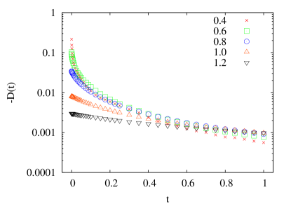
Figure 1: (Color online) Minus ${\cal D}(t)$ as a function of the interpolation parameter $t$ (both in logarithmic scale) for $N=1024$ and temperatures $0.4,0.6,\ldots,1.2$.

The right hand side of equation 6 can be evaluated with Monte Carlo simulation. I use the Parallel Tempering algorithm, with $T\in[0.4,1.3]$ and uniform $\Delta T=0.025$. A total of $2\ 10^{5}$ sweeps of the algorithm was used for every disorder sample. The quenched couplings have a binary distribution in order to speed up the computer program (as shown in reference PRS1 , the leading finite size correction is the same for the binary and Gaussian couplings). Systems of sizes $N$ from $128$ to $1024$ have been simulated with $128$ disorder samples for each system size (but for $N=1024$, where I used $196$ samples). The integration over $t$ was done with the trapezoidal rule, with $39$ non uniformly spaced points. Integrating with only half of the points makes a very small effect on the integrand (smaller than the estimated statistical error).

Figure 1 shows the integrand $D(t)$ as a function of $t$ for the largest system and several temperatures. The integrand is concentrated around $t=0$, and I have chosen the discretization of $t$ accordingly. One notices that ${\cal D}(t=0)$ is more and more negative as $T$ decreases, as predicted by the formula ${\cal D}(t=0)=-\overline{<(q_{12})^{2}>}$, and that ${\cal D}(t=1)$ is weakly dependent on $T$, as expected from the identity ${\cal D}(t=1)={1}/(N-1)(\overline{<(q_{12})^{2}>}-1)$, which is weakly dependent on $T$ (for not too small T’s) since $\overline{<(q_{12})^{2}>}$ is small compared to one.

In the low $T$ phase, a remarkable scaling is observed if one plots the ratio ${{\cal D}(t)}/{D(t=0)}$ as a function of $tN^{2/3}$, as shown in figures 2. It means that, to a good approximation, one has ${\cal D}(t)/{\cal D}(0)=F(tN^{2/3})$, with $F(x)$ decaying faster than $1/x$ for large $x$, making the integral in equation 6 converge. One has accordingly in the low $T$ phase $f_{N}-f_{\infty}\propto 1/N^{2/3}$. A temperature independent exponent $2/3$ for the free energy is in contradiction with the claims of KC that the internal energy scales like $e_{N}-e_{\infty}\propto 1/N^{x(T)}$, with an exponent $x(T)$ that is compatible with $2/3$ for both $T=0$ and $T_{c}$ but reaches a minimum $\approx 0.54$ between. The results of referenceKC are based however on Monte Carlo simulations of relatively small systems with $N$ up to $196$. Analyzing the data for the internal energy produced during the simulation of referenceBM , witch include systems with up to $4096$ spins, one findsmoi an exponent that is much closer to $2/3$, with deviations that are presumably explained by the proximity of the critical point and by the very slow convergence of the expansion of $e_{N}-e_{\infty}$ in inverse powers of $1/N$ (at $T_{c}$, the expansion parameter isPRS1 $1/N^{1/3}$).

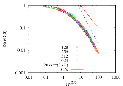
Figure 2: (Color online) ${{\cal D}(t)}/{D(t=0)}$ as a function of $tN^{2/3}$ (both in logarithmic scale), for $T=0.6$. The orange line (full line) shows the $1/x$ behavior, the blue line (dotted line) shows the $1/x^{3/2}$ behavior. Clearly $D(t)$ grows faster than $1/x$ for large $x$. The precise behavior of ${\cal D}(t)$ is not essential for my argument, as soon as it decays faster than $1/x$.

The situation is different at $T_{c}$, as shown in figure 3, the ratio ${{\cal D}(t)}/{D(t=0)}$ scales with a different exponent, namely like $F(tN^{1/3})$, with a large $x$ behavior compatible with $F(x)\propto 1/x$ (Although much larger system sizes would be needed in order to be sure that the system really approaches this asymptotic behavior). This is in agreement with formula 4 (In this model one has $\beta/\nu=2$). The data presented at $T_{c}$ (Figures 3 and 5) include the results of an additional simulation of a system with $N=2048$ sites, limited to the (cheap to simulate) paramagnetic phase, with $T\in[1.0,1.3]$, $\Delta T=0.025$, with 128 disorder samples, and a $15$ points discretization of $t$.

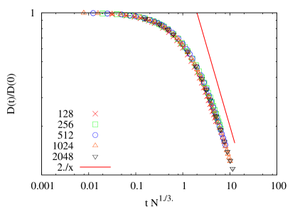
Figure 3: (Color online) ${{\cal D}(t)}/{D(t=0)}$ as a function of $tN^{1/3}$ (both in logarithmic scale), for $T=T_{c}$. The orange line (straight line) shows the expected $1/x$ behavior, in order to guide the eyes.

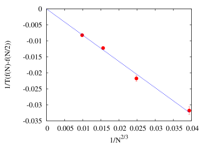
Figure 4: (Color online) Numerical data for $(f_{N}-f_{N/2})/T$ as a function of $1/N^{2/3}$, together with a numerical fit to the data of the form $(f_{N}-f_{N/2})/T=-A/N^{2/3}$, with $A=0.82\pm 0.02$ (blue dotted line). Here $T=0.4$, $N=128,256,512\ {\rm and}\ 1024$.

Figure 4 shows, as a function of $1/N^{2/3}$, my estimates, after integrating numerically equation 6, of $(f_{N}-f_{N/2})/T$ at $T=0.4$, compared to the result of a linear fit $(f_{N}-f_{N/2})/T=-A/N^{-2/3}$, with $A=0.82\pm 0.02$ and $\chi^{2}=4.9$. The agreement is good within estimated statistical errors. A similar agreement is obtained for other values of $T$ in the spin glass phase (e.g. $A=0.39\pm 0.01$ with $\chi^{2}=3.6$ for $T=0.6$, and $A=0.18\pm 0.01$ with $\chi^{2}=33$ - a large value presumably related to the proximity of the critical point - for $T=0.8$). Figure 5 shows my estimates for $(f_{N}-f_{N/2})/T$ at $T_{c}$ as a function of $1/N$, together with the prediction of equation 4. A good agreement (with $\chi^{2}=4.3$ if one excludes the $N=128$ data from the fit) is obtained using the value $1/N_{0}=7.8\pm 0.2$, namely $f_{(-1)}=\ln(7.8)/12=0.17\ldots$, within the range of results presented by Parisi, Ritort and Slanina PRS1 .

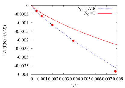
Figure 5: (Color online) Numerical data for $(f_{N}-f_{N/2})/T$ as a function of $1/N$, together with the behavior implied by the equation: $f_{N}/T=f_{\infty}/T+1/(12N)\ln{N/N_{0}}$. The orange line (full line) is drawn with the value $N_{0}=1$. The blue line (dotted line) is drawn with the value $1/7.8$, from a fit to the data. Here $T=1$, $N=128,256,\ldots,2048$.

In conclusion, I have shown that the Guerra–Toninelli interpolation provides an efficient method to evaluate numerically the finite size corrections to the free energy of the Sherrington–Kirkpatrick model. The integrand ${\cal D}(t)$ exhibits a remarkable scaling as a function of the interpolation parameter $t$ and system size $N$. At the critical temperature, the results for the free energy are in agreement with the predicted $(1/12N)\ln(N/N_{0})$ leading behavior of the finite size corrections, and give the estimate $N_{0}\approx 1/7.8$. In the low temperature phase, the results indicate that the leading corrections behave like $N^{-2/3}$ for both the internal energy and the free energy of the model.

I Acknowledgments

This work originates from a discussion with Giorgio Parisi. I thank him for his enlightening advises. I also acknowledge email exchanges with Frantisek Slanina, Andrea Crisanti, Ian Campbell and Helmut Katzgraber. The simulation was performed at CCRT, the CEA computer center at Bruyères-le-Châtel, using $\approx 32000$ hours of $1.25$ GHz alpha EV68.

References

- (1) G. Parisi, F. Ritort and F. Slanina, J. Phys A 26 247 (1992).
- (2) G. Parisi, F. Ritort and F. Slanina, J. Phys A 26, 3775 (1993).
- (3) M. A. Moore, cond-mat/0508087.
- (4) D. Sherrington, and S. Kirkpatrick, Phys. Rev. Lett 35 1792 (1975).
- (5) M. Talagrand, Spin Glasses: a challenge for mathematicians. Mean field theory and cavity method, Springer Verlag, Berlin (2003).
- (6) A. J. Bray and M. A. Moore, Phys. Rev. Lett 41 1068 (1978).
- (7) M. Palassini, PhD thesis, 2000 (unpublished).
- (8) M. Palassini, cond-mat/0307713.
- (9) J.-P. Bouchaud, F. Krzakala, and O. Martin, Phys. Rev. B 68, 224404 (2003).
- (10) S. Boettcher, Eur. Phys. J. B 31, 29 (2003); S. Boettcher, Eur. Phys. J. B 46, 501 (2005).
- (11) H. G. Katzgraber, M. Körner, F. Liers, M. Jünger and A. K. Hartmann, Phys. Rev. B 72, 094421 (2005).
- (12) A. Andreanov, F. Barbieri and O. Martin, Eur. Phys. J. B 41, 365 (2004).
- (13) H. G. Katzgraber, and I. A. Campbell, Phys. Rev. B 68, 180402(R) (2003).
- (14) G. Guerra and F. L. Toninelli, Commun. Math. Phys. 230 1, 71 (2002).
- (15) A. Billoire and E. Marinari, Europhys. Lett. 60, (2002).
- (16) A. Billoire, in “Rugged Free Energy Landscapes”, Springer Lecture Notes in Physics, editted by W. Janke, in preparation.