Functional renormalization group with vacuum expectation values and spontaneous symmetry breaking

Abstract

We generalize our recently developed super-field functional renormalization group (RG) method involving both Fermi and Bose fields [F. Schütz, L. Bartosch, and P. Kopietz, Phys. Rev. B 72, 035105 (2005)] to include the possibility that some bosonic components of the field have a finite vacuum expectation value. We derive an exact hierarchy of flow equations for the one-line irreducible vertices and the vacuum expectation value of the field. We apply our method to an interacting Fermi system where the interaction can be decoupled in the zero-sound channel and is then mediated by a collective bosonic field. The vacuum expectation value of the zero-frequency and zero-momentum component of the bosonic field is then closely related to the fermionic density. This can be exploited to calculate the compressibility of the interacting system. By using a cutoff in the bosonic propagator, the RG can be set up such that the self-consistent Hartree approximation is imposed as initial condition for the RG flow and the corrections to this approximation are generated as the remaining degrees of freedom are successively eliminated by the RG procedure.

1 Introduction

Recently, we have proposed (in collaboration with L. Bartosch) a new formulation of the functional renormalization group approach to interacting Fermi systems which is based on the explicit introduction of collective bosonic fields representing the relevant collective fluctuations via a suitable Hubbard-Stratonovich transformation [1]. In contrast to the conventional renormalization group (RG) approach to quantum critical phenomena pioneered by Hertz [2], in our approach the Fermi fields are not completely integrated out, but the RG flow of the coupled Fermi-Bose theory is derived using the functional RG equation for the generating functional of the one-line irreducible vertices [3, 4]. A similar strategy has recently been adopted by Baier, Bick and Wetterich [5]. However, on the technical level our formulation differs from that of Ref. [5]. In particular, we succeeded in introducing the RG cutoff parameter $\Lambda$ in such a way that the asymptotic Ward identities underlying the exact solubility of the one-dimensional Tomonaga-Luttinger model are preserved. This has enabled us to solve the infinite hierarchy of flow equations of the coupled Fermi-Bose theory and reproduce the exact solution for the single-particle Green function of the Tomonaga-Luttinger model entirely within the framework of the RG.

As pointed out in Ref. [1], our method should be especially convenient to study spontaneous symmetry breaking in interacting Fermi systems provided that the order parameter can be defined in terms of the vacuum expectation value of a suitable bosonic field. However, the exact RG flow equations in the form given in Ref. [1] are only valid as long as the fields do not have finite vacuum expectation values. We present here a generalization of the RG flow equations derived in Ref. [1] which explicitly allows for finite vacuum expectation values of one or several components of the fields. Note that this does not necessarily mean that some symmetry is spontaneously broken (see Sec. 4).

Previously, several authors have studied spontaneous symmetry breaking in interacting Fermi systems within the framework of the functional RG [6, 7, 8]. However, in these works a purely fermionic version of the functional RG has been used. In view of the bosonic nature of the order parameter field in interacting Fermi systems, a formulation where the flow of the vacuum expectation value of the order parameter field appears explicitly in the exact hierarchy of flow equations seems to be more advantageous, in particular in systems where the fluctuations of the order parameter field are controlled by a non-Gaussian fixed-point.

2 Exact RG flow equations with finite vacuum expectation values

In this section we consider a general Euclidean action $S[\Phi]=S_{0}[\Phi]+S_{1}[\Phi]$ involving some multi-component field $\Phi_{\alpha}$ which can have fermionic and bosonic components. The index $\alpha$ is a super-label for all quantities that are necessary to specify the fields, such as frequency, momentum, spin, and field-type. We write the quadratic part $S_{0}[\Phi]$ of the action as

$$S_{0}[\Phi]=-\frac{1}{2}\left(\Phi,\left[{\bf G}_{0}\right]^{-1}\Phi\right)=-\frac{1}{2}\int_{\alpha}\int_{\alpha^{\prime}}\Phi_{\alpha}\left[{\bf G}_{0}\right]^{-1}_{\alpha\alpha^{\prime}}\Phi_{\alpha^{\prime}}\,,$$ (1)

where ${\bf G}_{0}$ is a matrix in all indices and the symbol $\int_{\alpha}$ denotes integration over the continuous components and summation over the discrete components of the super-index $\alpha$. At this point it is not necessary to specify the interaction part $S_{1}[\Phi]$, which can contain terms describing interactions between more than two particles and couplings between the fermionic and bosonic components of the super-field $\Phi_{\alpha}$. The generating functional $\mathcal{G}_{c}[J]$ of the connected Green functions can be defined as the following functional integral,

$$e^{\mathcal{G}_{c}[J]}=\frac{1}{\mathcal{Z}_{0}}\int\!\!D\Phi\,\,e^{-S_{0}-S_{1}+(J,\Phi)}\;,$$ (2)

where $J_{\alpha}$ are super-sources associated with the super-fields, and we use the compact notation

$$(J,\Phi)=\int_{\alpha}J_{\alpha}\Phi_{\alpha}\;.$$ (3)

The partition function $\mathcal{Z}_{0}$ of the non-interacting system can be written as the Gaussian integral

$$\mathcal{Z}_{0}=\int\!\!D\Phi\,\,e^{-S_{0}}\,.$$ (4)

Suppose now that at least one of the components of the super-field $\Phi_{\alpha}$ has a finite expectation value (vacuum expectation value) even for vanishing source fields $J$,

$$\left.\frac{\delta{\cal{G}}_{c}[J]}{\delta J_{\alpha}}\right|_{J\to 0}=\left.\langle\Phi_{\alpha}\rangle\right|_{J\to 0}\equiv\Phi_{\alpha}^{0}\neq 0\;.$$ (5)

We now derive an exact hierarchy for RG flow equations for the one-line irreducible vertices and for the vacuum expectation value. The exact hierarchy obtained in [1] is only applicable if none of the field components has a finite vacuum expectation value. To generalize the hierarchy of flow equations, we proceed as usual and introduce a cutoff $\Lambda$ into the theory by modifying ${\bf G}_{0}$ such that the long-wavelength and low-energy modes are suppressed. At this point it is not necessary to specify the precise cutoff procedure. Differentiating Eq. (2) with respect to $\Lambda$ we obtain [1]

$$\partial_{\Lambda}{\cal{G}}_{c}=\frac{1}{2}\left(\frac{\delta\mathcal{G}_{c}}{\delta J},[\partial_{\Lambda}\mathbf{G}_{0}^{-1}]\frac{\delta\mathcal{G}_{c}}{\delta J}\right)+\frac{1}{2}\mathrm{Tr}\left([\partial_{\Lambda}\mathbf{G}_{0}^{-1}]\left[\frac{\delta^{(2)}\mathcal{G}_{c}}{\delta J\delta J}\right]^{T}\right)-\partial_{\Lambda}\ln\mathcal{Z}_{0}\,,$$ (6)

where we have defined the following matrix in the super-indices,

$$\left[\frac{\delta^{(2)}\mathcal{G}_{c}}{\delta J\delta J}\right]_{\alpha\alpha^{\prime}}=\frac{\delta^{(2)}\mathcal{G}_{c}}{\delta J_{\alpha}\delta J_{\alpha^{\prime}}}\;.$$ (7)

To discuss symmetry breaking, it is more convenient to consider the Legendre transform of ${\cal{G}}_{c}[J]$,

$${\cal{L}}[\Phi]=(J[\Phi],\Phi)-{\cal{G}}_{c}[J[\Phi]]$$ (8)

which has an extremum at $\Phi_{\alpha}=\Phi_{\alpha}^{0}$,

$$\left.\frac{\delta{\cal{L}}[\Phi]}{\delta\Phi_{\alpha}}\right|_{\Phi=\Phi^{0}}=0\;.$$ (9)

Actually, the field $\Phi$ in Eqs. (8) and (9) denotes the expectation value of the field $\Phi$ in Eq. (2). To simplify the notation, we use the same symbol for both quantities; it is understood that from now on we redefine $\langle\Phi_{\alpha}\rangle\rightarrow\Phi_{\alpha}$. In order to derive the exact RG flow equations of the one-line irreducible vertices $\Gamma^{(n)}_{\alpha_{1},\dots,\alpha_{n}}$ in the presence of a finite vacuum expectation value $\Phi^{0}$, we consider the flow equation for the generating functional

$$\Gamma[\Phi]={\cal{L}}[\Phi]+\frac{1}{2}(\Delta\Phi,{\bf{G}}_{0}^{-1}\Delta\Phi)\;,$$ (10)

where $\Delta\Phi_{\alpha}=\Phi_{\alpha}-\Phi_{\alpha}^{0}$. Note that by construction $\Gamma[\Phi]$ is also extremal at $\Phi_{\alpha}=\Phi_{\alpha}^{0}$,

$$\left.\frac{\delta\Gamma[\Phi]}{\delta\Phi_{\alpha}}\right|_{\Phi=\Phi^{0}}=0\;.$$ (11)

The one-line irreducible vertices $\Gamma^{(n)}_{\alpha_{1},\dots,\alpha_{n}}$, which depend implicitly on the vacuum expectation value $\Phi^{0}$, are then defined via the functional Taylor expansion around $\Phi^{0}$ (see, e.g., [9] and references therein),

$$\Gamma[\Phi]=\sum_{n=0}^{\infty}\frac{1}{n!}\int_{\alpha_{1}}\dots\int_{\alpha_{n}}\Gamma^{(n)}_{\alpha_{1},\dots,\alpha_{n}}\Delta\Phi_{\alpha_{1}}\cdot\ldots\cdot\Delta\Phi_{\alpha_{n}}\;.$$ (12)

Using Eqs. (8), (10) and $\delta{\cal{G}}_{c}/\delta J_{\alpha}=\Phi_{\alpha}$, we obtain the exact flow equation

$$\partial_{\Lambda}\Gamma=-\frac{1}{2}\mathrm{Tr}\left([\partial_{\Lambda}\mathbf{G}_{0}^{-1}]\left[\frac{\delta^{(2)}\mathcal{G}_{c}}{\delta J\delta J}\right]^{T}\right)+\partial_{\Lambda}\ln\mathcal{Z}_{0}$$

$$-(\Delta\Phi,\partial_{\Lambda}[\mathbf{G}_{0}^{-1}\Phi^{0}])-\frac{1}{2}(\Phi^{0},[\partial_{\Lambda}\mathbf{G}_{0}^{-1}]\Phi^{0})\;.$$ (13)

Introducing the matrices $\mathbf{\Sigma}$, $\mathbf{U}$, $\mathbf{G}$ and $\dot{\mathbf{G}}$ via

$$\mathbf{\Sigma}=\left[\frac{\delta^{(2)}\Gamma}{\delta\Phi\delta\Phi}\right]_{\Phi=\Phi^{0}}^{T}\;,$$ (14)

$$\mathbf{U}=\left[\frac{\delta^{(2)}\Gamma}{\delta\Phi\delta\Phi}\right]^{T}-\left[\frac{\delta^{(2)}\Gamma}{\delta\Phi\delta\Phi}\right]_{\Phi=\Phi^{0}}^{T}=\left[\frac{\delta^{(2)}\Gamma}{\delta\Phi\delta\Phi}\right]^{T}-\mathbf{\Sigma}\;,$$ (15)

$$\mathbf{G}^{-1}=\mathbf{G}_{0}^{-1}-\mathbf{\Sigma}\,,$$ (16)

$$\dot{\mathbf{G}}=-\mathbf{G}\partial_{\Lambda}[\mathbf{G}_{0}^{-1}]\mathbf{G}=[\mathbf{1}-\mathbf{G}_{0}\mathbf{\Sigma}]^{-1}\left(\partial_{\Lambda}\mathbf{G}_{0}\right)[\mathbf{1}-\mathbf{\Sigma}\mathbf{G}_{0}]^{-1}\;,$$ (17)

we may rewrite Eq. (13) as follows,

$$\partial_{\Lambda}\Gamma = -\frac{1}{2}\mathrm{Tr}\left[\mathbf{Z}\dot{\mathbf{G}}^{T}\mathbf{U}^{T}\left\{\mathbf{1}-\mathbf{G}^{T}\mathbf{U}^{T}\right\}^{-1}\right]-(\Delta\Phi,\partial_{\Lambda}[\mathbf{G}_{0}^{-1}\Phi^{0}])$$ (18)

$$-\frac{1}{2}\mathrm{Tr}\left[\mathbf{Z}\dot{\mathbf{G}}_{0}^{T}\mathbf{\Sigma}^{T}\left\{\mathbf{1}-\mathbf{G}_{0}^{T}\mathbf{\Sigma}^{T}\right\}^{-1}\right]-\frac{1}{2}(\Phi^{0},[\partial_{\Lambda}\mathbf{G}_{0}^{-1}]\Phi^{0})\;,$$

where $[{\bf Z}]_{\alpha\beta}=\delta_{\alpha,\beta}\zeta_{\alpha}$ with $\zeta_{\alpha}=\pm 1$ depending on whether $\Phi_{\alpha}$ is a bosonic or fermionic field. To obtain the flow equations for the vertices, we should take into account that $\Phi^{0}$ depends on $\Lambda$, so that the derivative of Eq. (12) with respect to $\Lambda$ yields

$$\partial_{\Lambda}\Gamma=\sum_{n=0}^{\infty}\frac{1}{n!}\int_{\alpha_{1}}\dots\int_{\alpha_{n}}\partial_{\Lambda}\Gamma^{(n)}_{\alpha_{1},\dots,\alpha_{n}}\Delta\Phi_{\alpha_{1}}\cdot\ldots\cdot\Delta\Phi_{\alpha_{n}}$$

$$-\sum_{n=0}^{\infty}\frac{1}{n!}\int_{\alpha}\int_{\alpha_{1}}\dots\int_{\alpha_{n}}\Gamma^{(n+1)}_{\alpha,\alpha_{1},\dots,\alpha_{n}}(\partial_{\Lambda}\Phi^{0}_{\alpha})\Delta\Phi_{\alpha_{1}}\cdot\ldots\cdot\Delta\Phi_{\alpha_{n}}\;.$$ (19)

Equating the right-hand sides of Eq. (18) and (19) we obtain the flow equations for the one-line irreducible vertices. The vertex $\Gamma^{(0)}$ with no external legs is the interaction correction to the grand canonical potential. Its flow equation is

$$\partial_{\Lambda}\Gamma^{(0)}=-\frac{1}{2}\mathrm{Tr}\left[\mathbf{Z}\dot{\mathbf{G}}_{0}^{T}\mathbf{\Sigma}^{T}\left\{\mathbf{1}-\mathbf{G}_{0}^{T}\mathbf{\Sigma}^{T}\right\}^{-1}\right]-\frac{1}{2}(\Phi^{0},[\partial_{\Lambda}\mathbf{G}_{0}^{-1}]\Phi^{0})-\!\!\int_{\alpha}(\partial_{\Lambda}\Phi^{0}_{\alpha})\Gamma^{(1)}_{\alpha}.$$ (20)

The flow equation for the vertex $\Gamma^{(1)}_{\alpha}$ with one external leg is

$$\partial_{\Lambda}\Gamma^{(1)}_{\alpha}=-\frac{1}{2}\mathrm{Tr}\left[\mathbf{Z}\dot{\mathbf{G}}^{T}\mathbf{\Gamma}^{(3)T}_{\alpha}\right]-\int_{\alpha^{\prime}}[\mathbf{G}^{-1}]_{\alpha\alpha^{\prime}}(\partial_{\Lambda}\Phi^{0}_{\alpha^{\prime}})-\int_{\alpha^{\prime}}[\partial_{\Lambda}\mathbf{G}_{0}^{-1}]_{\alpha\alpha^{\prime}}\Phi^{0}_{\alpha^{\prime}}\;,$$ (21)

and the flow equations for the vertices $\Gamma^{(n)}$ with $n\geq 2$ can be written in closed form as follows,

$$\partial_{\Lambda}{\Gamma}^{(n)}_{\alpha_{1},\dots,\alpha_{n}}=\int_{\alpha}(\partial_{\Lambda}\Phi_{\alpha}^{0})\Gamma^{(n+1)}_{\alpha\alpha_{1}\ldots\alpha_{n}}-\frac{1}{2}\sum\limits_{l=1}^{\infty}\sum\limits_{m_{1},\dots,m_{l}=1}^{\infty}\delta_{n,m_{1}+\ldots+m_{l}}\,$$

$$\times{\cal{S}}_{\alpha_{1},\dots,\alpha_{m_{1}};\alpha_{m_{1}+1},\dots,\alpha_{m_{1}+m_{2}};\dots;\alpha_{m_{1}+\ldots+m_{l-1}+1},\dots,\alpha_{n}}\Big{\{}$$

$$~{}~{}~{}~{}~{}~{}~{}~{}\mathrm{Tr}\left[\mathbf{Z}\dot{\mathbf{G}}^{T}\mathbf{\Gamma}^{(m_{1}+2)\,T}_{\alpha_{1},\dots,\alpha_{m_{1}}}\mathbf{G}^{T}\mathbf{\Gamma}^{(m_{2}+2)\,T}_{\alpha_{m_{1}+1},\dots,\alpha_{m_{1}+m_{2}}}\cdot\dots\cdot\mathbf{G}^{T}\mathbf{\Gamma}^{(m_{l}+2)\,T}_{\alpha_{m_{1}+\ldots+m_{l-1}+1},\dots,\alpha_{n}}\right]\Big{\}}\,,$$ (22)

where the matrices $\mathbf{\Gamma}^{(n+2)}_{\alpha_{1},\dots,\alpha_{n}}$ are defined as follows

$$[\mathbf{\Gamma}^{(n+2)}_{\alpha_{1},\dots,\alpha_{n}}]_{\alpha\alpha^{\prime}}=\Gamma^{(n+2)}_{\alpha\alpha^{\prime}\alpha_{1}\dots\alpha_{n}}\;.$$ (23)

The operator ${\cal{S}}$ symmetrizes the expression in curly brackets with respect to indices on different correlation functions, i.e., it generates all permutations of the indices with appropriate signs, counting expressions only once that are generated by permutations of indices on the same vertex. More precisely the action of ${\cal{S}}$ is given by ($m=\sum_{i=1}^{l}m_{i}$)

$${\cal{S}}_{\alpha_{1},\dots,\alpha_{m_{1}};\dots;\alpha_{m-m_{l}+1},\dots,\alpha_{m}}\{A_{\alpha_{1},\dots,\alpha_{m}}\}=\frac{1}{\prod_{i}m_{i}!}\sum_{P}\mathrm{sgn}_{\zeta}(P)\,A_{\alpha_{P(1)},\dots,\alpha_{P(m)}}\,,$$ (24)

where $P$ denotes a permutation of $\{1,\dots,m\}$ and $\mathrm{sgn}_{\zeta}$ is the sign created by permuting field variables according to the permutation $P$, i.e.,

$$\Phi_{\alpha_{1}}\cdot\ldots\cdot\Phi_{\alpha_{m}}=\mathrm{sgn}_{\zeta}(P)\,\Phi_{\alpha_{P(1)}}\cdot\ldots\cdot\Phi_{\alpha_{P(m)}}\;.$$ (25)

We now adjust the flowing vacuum expectation value $\Phi^{0}$ such that for any value of the cutoff $\Lambda$ the vertex $\Gamma^{(1)}_{\alpha}$ vanishes. In this case $\Phi^{0}$ can be identified with the flowing extremum of the effective potential. The above equations (20) and (21) can be further simplified if we choose the inverse free propagator ${\bf{G}}_{0}^{-1}$ such that

$${\bf{G}}_{0}^{-1}\Phi^{0}=0\;,\qquad\;[\partial_{\Lambda}{\bf{G}}_{0}^{-1}]\Phi^{0}=0\;.$$ (26)

We assume that this can always be achieved, if necessary by including appropriate counter-terms in the Gaussian part of the action. Then the last two terms on the right-hand sides of Eqs.(20) and (21) vanish and the latter equation becomes

$$\int_{\alpha}[\mathbf{\Sigma}]_{\alpha_{1}\alpha}\partial_{\Lambda}\Phi^{0}_{\alpha}=\frac{1}{2}\mathrm{Tr}\left[\mathbf{\Gamma}^{(3)}_{\alpha_{1}}\dot{\mathbf{G}}\right]\;,$$ (27)

which relates the RG flow of the vacuum expectation value $\Phi^{0}_{\alpha}$ to the irreducible self-energy $\mathbf{\Sigma}$ and the three-legged vertex $\Gamma^{(3)}$. Diagrammatic representations of the flow equations for $\Gamma^{(n)}$ with $n=1,2,3,4$ are shown in Fig. 1.

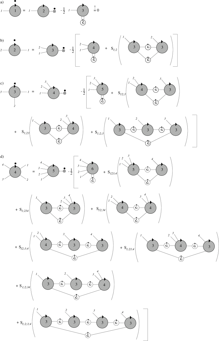
Figure 1: Diagrammatic representations of the exact RG flow equations for the first few one-line irreducible vertices: (a) $\Gamma^{(1)}$, (b) $\Gamma^{(2)}$, (c) $\Gamma^{(3)}$, (d) $\Gamma^{(4)}$. Shaded circles represent one-line irreducible vertex functions, whereas circles labeled by ${\bf G}$ and $\dot{\bf G}$ represent the full Green function and the single scale propagator defined in Eqs. (16) and (17) respectively. The small dotted circle with a cross denotes the change $\partial_{\Lambda}\Phi^{0}$ of the vacuum expectation value. The action of the symmetrization operator $\mathcal{S}$ is defined in Eq. (24). The arrow on the circles indicates the order of the indices on the corresponding correlation function, which is important to keep track of the signs, when Fermi fields are present.

3 Flow equations in the symmetry broken phase of the Ising model

Before applying the general equations derived above to quantum systems involving both fermions and bosons, it is instructive to examine these equations in the context of classical $\varphi^{4}$-theory in $D$ dimensions, which describes the critical properties of the $D$-dimensional Ising model. In this case our super-field $\Phi$ has only a single component $\varphi$ and the super-index $\alpha$ labels momenta $\bm{k}$ (or, alternatively, points $\bm{r}$ in $D$-dimensional space). Our initial action is $S[\varphi]=S_{0}[\varphi]+S_{1}[\varphi]$, where

$$S_{0}[\varphi]=\frac{1}{2}\int_{\bm{k}}G_{0}^{-1}(\bm{k})\varphi_{-\bm{k}}\varphi_{\bm{k}}\;,$$ (28)

and the interaction part is

$$S_{1}[\varphi]=\frac{r_{0}}{2}\int_{\bm{k}}\varphi_{-\bm{k}}\varphi_{\bm{k}}+\frac{u_{0}}{4!}\int_{\bm{k}_{1}}\ldots\int_{\bm{k}_{4}}(2\pi)^{D}\delta(\sum_{i=1}^{4}\bm{k}_{i})\varphi_{\bm{k}_{1}}\cdots\varphi_{\bm{k}_{4}}\;.$$ (29)

Here $\int_{\bm{k}}=\frac{1}{V}\sum_{\bm{k}}\to\int\frac{d^{D}k}{(2\pi)^{D}}$, for $V\to\infty$, where $V$ is the volume of the system. Furthermore, using a sharp cutoff in momentum space for simplicity, the cutoff-dependent free propagator is given by

$$G_{0}(\bm{k})=\frac{\Theta(\Lambda<|\bm{k}|<\Lambda_{0})}{c_{0}\bm{k}^{2}}\;,$$ (30)

where $\Theta(\Lambda<|\bm{k}|<\Lambda_{0})$ is unity if $\Lambda<|\bm{k}|<\Lambda_{0}$ and vanishes otherwise. For the Ising model on a $D$-dimensional hypercubic lattice with lattice spacing $a$ the bare parameters are $c_{0}=(2D)^{-1}$ and $r_{0}=a^{-2}(T-T_{c}^{\rm MF})/T_{c}^{\rm MF}$, where $T_{c}^{\rm MF}$ is the mean-field result for the critical temperature. In the symmetry broken phase the $\bm{k}=0$ Fourier component of the field has a finite expectation value. It is then natural to shift

$$\varphi_{\bm{k}}=\varphi^{0}_{\bm{k}}+\Delta\varphi_{\bm{k}}\;,\qquad\varphi^{0}_{\bm{k}}=(2\pi)^{D}\delta(\bm{k})M\;.$$ (31)

For the Ising model, the parameter $M$ has the physical meaning of the magnetization per unit volume. Note that $G_{0}^{-1}(\bm{k})\varphi^{0}_{\bm{k}}=0$, so that the condition (26) is satisfied. This is the reason why we have included the quadratic part of the action proportional to $r_{0}$ into the definition of the interaction term in Eq. (29). Our initial action then takes the form $S[\varphi]=S_{0}[\Delta\varphi]+S_{1}[\varphi^{0};\Delta\varphi]$ with

$$S_{1}[\varphi^{0};\Delta\varphi] = S_{1}[\varphi\rightarrow\varphi^{0}+\Delta\varphi]=V\Bigr{[}\frac{r_{0}}{2}M^{2}+\frac{u_{0}}{4!}M^{4}\Bigr{]}$$

$$+ \Gamma^{(1)}_{0}\Delta\varphi_{0}+\frac{1}{2}\int_{\bm{k}}\Gamma^{(2)}_{0}(\bm{k})\Delta\varphi_{-\bm{k}}\Delta\varphi_{\bm{k}}$$

$$+ \frac{1}{3!}\int_{\bm{k}_{1}}\int_{\bm{k}_{2}}\int_{\bm{k}_{3}}(2\pi)^{D}\delta(\sum_{i=1}^{3}\bm{k}_{i})\Gamma^{(3)}_{0}(\bm{k}_{1},\bm{k}_{2},\bm{k}_{3})\Delta\varphi_{\bm{k}_{1}}\Delta\varphi_{\bm{k}_{2}}\Delta\varphi_{\bm{k}_{3}}$$

$$+ \frac{1}{4!}\int_{\bm{k}_{1}}\ldots\int_{\bm{k}_{4}}(2\pi)^{D}\delta(\sum_{i=1}^{4}\bm{k}_{i})\Gamma^{(4)}_{0}(\bm{k}_{1},\bm{k}_{2},\bm{k}_{3},\bm{k}_{4})\Delta\varphi_{\bm{k}_{1}}\Delta\varphi_{\bm{k}_{2}}\Delta\varphi_{\bm{k}_{3}}\Delta\varphi_{\bm{k}_{4}}\;,$$

where the bare vertices now depend on $M$,

$$\Gamma^{(1)}_{0} = r_{0}M+\frac{u_{0}}{6}M^{3}\;,$$ (33)

$$\Gamma^{(2)}_{0}(\bm{k}) = r_{0}+\frac{u_{0}}{2}M^{2}\;,$$ (34)

$$\Gamma^{(3)}_{0}(\bm{k}_{1},\bm{k}_{2},\bm{k}_{3}) = u_{0}M\;,$$ (35)

$$\Gamma^{(4)}_{0}(\bm{k}_{1},\bm{k}_{2},\bm{k}_{3},\bm{k}_{4}) = u_{0}\;.$$ (36)

We now require that $\Gamma^{(1)}_{0}=0$, so that the initial value $M_{0}$ of the order parameter in our functional RG is the minimum of the effective potential in the Landau approximation,

$$M_{0}=\left\{\begin{array}[]{cc}0&\mbox{for $r_{0}>0$}\\ \sqrt{-6r_{0}/u_{0}}&\mbox{for $r_{0}<0$}\end{array}\right.\;.$$ (37)

Note that for $r_{0}<0$ we have

$$\Gamma^{(2)}_{0}(\bm{k})=\frac{u_{0}}{3}M_{0}^{2}\;,$$ (38)

so that in this case the interaction part of our initial action can be written in real space as

$$S_{1}[\varphi]=\int d^{D}r\frac{u_{0}}{4!}[\varphi^{2}(\bm{r})-M_{0}^{2}]^{2}\;.$$ (39)

With a sharp cutoff in momentum space we obtain from Eq. (20) for the interaction correction to the grand canonical potential,

$$\partial_{\Lambda}\Gamma_{\Lambda}^{(0)}=-\frac{V}{2}\int_{\bm{k}}\delta(|\bm{k}|-\Lambda)\ln\left[\frac{c_{0}\Lambda^{2}+\Gamma^{(2)}_{\Lambda}(\bm{k})}{c_{0}\Lambda^{2}}\right]\;.$$ (40)

The order parameter flow equation (27) reduces to

$$(\partial_{\Lambda}M_{\Lambda})\Gamma_{\Lambda}^{(2)}(0)=-\frac{1}{2}\int_{\bm{k}}\dot{G}_{\Lambda}(\bm{k})\Gamma^{(3)}_{\Lambda}(\bm{k},-\bm{k},0)\;.$$ (41)

For a sharp cutoff in momentum space, we have

$${G}_{\Lambda}(\bm{k})=\frac{\Theta(\Lambda<|\bm{k}|<\Lambda_{0})}{c_{0}\bm{k}^{2}+\Gamma^{(2)}(\bm{k})}\;,$$ (42)

and hence

$$\dot{G}_{\Lambda}(\bm{k})=-\frac{\delta(|\bm{k}|-\Lambda)}{c_{0}\Lambda^{2}+\Gamma^{(2)}(\bm{k})}\;.$$ (43)

From Eq. (22), we obtain for the two-point vertex

$$\partial_{\Lambda}\Gamma^{(2)}_{\Lambda}(\bm{k})=\frac{1}{2}\int_{\bm{k}^{\prime}}\dot{G}_{\Lambda}(\bm{k}^{\prime})\Gamma^{(4)}_{\Lambda}(\bm{k}^{\prime},-\bm{k}^{\prime},\bm{k},-\bm{k})$$

$$-\int_{\bm{k}^{\prime}}\dot{G}_{\Lambda}(\bm{k}^{\prime}){G}_{\Lambda}(\bm{k}^{\prime}+\bm{k})\Gamma^{(3)}_{\Lambda}(\bm{k},-\bm{k}-\bm{k}^{\prime},\bm{k}^{\prime})\Gamma^{(3)}_{\Lambda}(-\bm{k}^{\prime},\bm{k}+\bm{k}^{\prime},-\bm{k})$$

$$+(\partial_{\Lambda}M_{\Lambda})\Gamma_{\Lambda}^{(3)}(\bm{k},-\bm{k},0)\;.$$ (44)

The above system of flow equations is exact but not closed. In order to obtain a closed system for the two-point vertex and the order parameter, it is necessary to express the vertices $\Gamma^{(3)}$ and $\Gamma^{(4)}$ in terms of $\Gamma^{(2)}$ and $M$. We now propose a simple polynomial truncation which is motivated by the generalized gradient expansion for the effective potential [9]. Guided by our initial conditions (35), (36) and (38), we truncate the above equations by substituting on the right-hand sides

$$\Gamma^{(2)}_{\Lambda}(\bm{k}) \approx \frac{u_{\Lambda}}{3}M_{\Lambda}^{2}\;,$$ (45)

$$\Gamma^{(3)}_{\Lambda}(\bm{k}_{1},\bm{k}_{2},\bm{k}_{3}) \approx u_{\Lambda}M_{\Lambda}\;,$$ (46)

$$\Gamma^{(4)}_{\Lambda}(\bm{k}_{1},\bm{k}_{2},\bm{k}_{3},\bm{k}_{4}) \approx u_{\Lambda}\;.$$ (47)

If we ignore the momentum-dependencies of the vertices also on the left-hand sides of the flow equations, this truncation amounts to approximating

$$\Gamma_{\Lambda}[\varphi]=\int d^{D}r\frac{u_{\Lambda}}{4!}[\varphi^{2}(\bm{r})-M_{\Lambda}^{2}]^{2}\;,$$ (48)

which is nothing but the quartic approximation to the effective potential in the symmetry broken phase to zeroth order in the gradient approximation [9]. In this approximation we obtain from Eq. (41) for the flow of the order parameter,

$$\partial_{\Lambda}M_{\Lambda}^{2}=-3\int_{\bm{k}}\dot{G}_{\Lambda}(\bm{k})\;,$$ (49)

while Eq. (44) reduces to

$$\partial_{\Lambda}u_{\Lambda}=-3u_{\Lambda}^{2}\int_{\bm{k}}\dot{G}_{\Lambda}(\bm{k})G_{\Lambda}(\bm{k})\;.$$ (50)

We shall not further analyze these equations, because they are completely equivalent to the RG flow equations discussed by Berges et al. [9] using the truncated effective potential (48) to zeroth order in the gradient expansion. Whether or not the polynomial truncation is justified is a different issue; according to Refs. [10, 11], this truncation fails to describe some important features of the symmetry breaking phenomenon. With the help of Eq. (44) one can easily go beyond this approximation. For example, we may solve this equation iteratively by substituting the truncation in Eqs. (45)–(47) only on the right-hand sides, retaining the momentum-dependence generated by the Green’s functions [12, 13]. From the momentum-dependent self-energy we can then obtain an estimate for the anomalous dimension. Having gained some confidence in our RG equations, we now focus on a more interesting problem involving both bosonic and fermionic degrees of freedom.

4 RG approach to interacting Fermions via partial bosonization in the zero-sound channel

In the approach developed in [1], tad-pole diagrams of the Hartree-type have not been considered due to the assumed overall charge neutrality of the system. For more general interactions, these diagrams do contribute and can lead to a non-vanishing expectation value of the field describing density fluctuations. In this section, this effect is treated with the formalism developed above for symmetry breaking.

We consider a system with a density-density interaction. After a Hubbard-Stratonovich transformation in the zero-sound channel the interaction is mediated by a real bosonic field $\varphi$ and the resulting action reads [1]

$$S[\bar{\psi},\psi,\varphi]=S_{0}[\bar{\psi},\psi]+S_{0}[\varphi]+S_{1}[\bar{\psi},\psi,\varphi]\;,$$ (51)

with the free parts

$$S_{0}[\bar{\psi},\psi]=-\sum_{\sigma}\int_{K}\bar{\psi}_{K\sigma}G^{-1}_{0,\sigma}(K)\psi_{K\sigma}$$ (52)

$$S_{0}[\varphi]=\frac{1}{2}\sum_{\sigma\sigma^{\prime}}\int_{\bar{K}}[F_{0}(\bar{K})^{-1}]_{\sigma\sigma^{\prime}}\varphi^{*}_{\bar{K}\sigma}\varphi_{\bar{K}\sigma^{\prime}}\;,$$ (53)

and the coupling between Fermi and Bose fields

$$S_{1}[\bar{\psi},\psi,\varphi]=i\sum_{\sigma}\int_{{K}}\int_{\bar{K}}\bar{\psi}_{K+\bar{K},\sigma}\psi_{K\sigma}\varphi_{\bar{K}\sigma}+\frac{1}{2\beta V}\sum_{\sigma,\sigma^{\prime}}[f_{0}^{-1}]^{\sigma\sigma^{\prime}}\varphi_{0\sigma}\varphi_{0\sigma^{\prime}}\,.$$ (54)

We use composite frequency-momentum indices $K=(i\omega,{\bm{k}})$ and $\bar{K}=(i\bar{\omega},{\bar{\bm{k}}})$ which include fermionic and bosonic momenta and Matsubara frequencies. The integration measure is $\int_{K}=\frac{1}{\beta V}\sum_{\omega,{\bm{k}}}$ and reduces to $\int\frac{d\omega}{2\pi}\frac{d^{D}k}{(2\pi)^{D}}$ in the zero-temperature and thermodynamic limit $\beta,V\to\infty$. The propagators are given by

$$G_{0,\sigma}(K)=\frac{\Theta(\Lambda_{F}<|\xi_{{\bm{k}}\sigma}-\Sigma_{\sigma}^{*}(i0,{\bm{k}}_{F})|/v_{0}<\Lambda_{F,0})}{i\omega-\xi_{{\bm{k}}\sigma}}\,,$$ (55)

$$F_{0,\sigma\sigma^{\prime}}(\bar{K})=[f^{-1}_{\bar{\bm{k}}}(1-\delta_{\bar{K},0}/(\beta V))]^{-1}_{\sigma\sigma^{\prime}}\Theta(\Lambda_{B}<|\bar{k}|<\Lambda_{B,0})\,,$$ (56)

with an arbitrary fermionic dispersion $\xi_{{\bm{k}}\sigma}=\epsilon_{{\bm{k}}\sigma}-\mu$ measured relative to the chemical potential $\mu$, the Fourier transformed interaction $f_{\bar{\bm{k}}}^{\sigma\sigma^{\prime}}$, and some average Fermi velocity $v_{0}$ which is introduced to give $\Lambda_{F}$ units of momentum. Here, $\Sigma^{*}=\Sigma^{\Lambda_{F}=\Lambda_{B}=0}$ is the self energy of the fully interacting system, which has to be introduced as a counter-term in order to scale toward the true Fermi surface [14]. We have allowed for the possibility of independent cutoffs on bosonic and fermionic degrees of freedom.

The Legendre transformation is performed for fermionic as well as bosonic fields, such that the resulting functional $\Gamma[\bar{\psi},\psi,\varphi]$ generates one-line irreducible vertices that are irreducible in the particle propagator as well as interaction lines [1]. At finite density, the bosonic field $\varphi$ acquires an expectation value and should be shifted according to $\varphi_{\bar{K}\sigma}=\varphi^{0}_{\bar{K}\sigma}+\Delta\varphi_{\bar{K}\sigma}$ with

$$\varphi^{0}_{\bar{K}\sigma}=-i\delta_{\bar{K},0}\bar{\varphi}_{\sigma}\,,\qquad\bar{\varphi}_{\sigma}=\sum_{\sigma^{\prime}}f_{0}^{\sigma\sigma^{\prime}}\rho_{\sigma^{\prime}}\,.$$ (57)

By integrating out the bosonic fields, it is straightforward to see that for $\Lambda_{F}=\Lambda_{B}=0$, the quantity $\rho_{\sigma}$ is the density of the interacting electron system in the spin channel $\sigma$, i.e., $\rho_{\sigma}=\int_{\bm{k}}\langle\hat{c}_{{\bm{k}}\sigma}^{+}\hat{c}_{{\bm{k}}\sigma}\rangle$, where $\hat{c}_{{\bm{k}}\sigma}$ is the usual second quantized fermion annihilation operator. The zero frequency and momentum parts of the interaction have not been included in $F_{0}$ to fulfill the property (26) of the free propagators. The functional Taylor expansion

$$\Gamma[\bar{\psi},\psi,\varphi]=\sum_{n=0}^{\infty}\sum_{m=0}^{\infty}\frac{1}{(n!)^{2}m!}\int_{K_{1}^{\prime}\sigma_{1}^{\prime}}\dots\int_{K_{n}^{\prime}\sigma_{n}^{\prime}}\int_{K_{1}\sigma_{1}}\dots\int_{K_{n}\sigma_{n}}\int_{\bar{K}_{1}\bar{\sigma}_{1}}\dots\int_{\bar{K}_{m}\bar{\sigma}_{m}}$$

$$\times\delta_{K^{\prime}_{1}+\ldots+K^{\prime}_{n},K_{1}+\ldots+K_{n}+\bar{K}_{1}+\ldots+\bar{K}_{m}}$$

$$\times\Gamma^{(2n,m)}(K^{\prime}_{1}\sigma_{1}^{\prime},\dots,K^{\prime}_{n}\sigma_{n}^{\prime};K_{1}\sigma_{1},\dots,K_{n}\sigma_{n};\bar{K}_{1}\bar{\sigma}_{1},\dots,\bar{K}_{m}\bar{\sigma}_{m})$$

$$\times\bar{\psi}_{K^{\prime}_{1}\sigma_{1}^{\prime}}\cdot\ldots\cdot\bar{\psi}_{K^{\prime}_{n}\sigma_{n}^{\prime}}\psi_{K_{1}\sigma_{1}}\cdot\ldots\cdot\psi_{K_{n}\sigma_{n}}\Delta\varphi_{\bar{K}_{1}\bar{\sigma}_{1}}\cdot\ldots\cdot\Delta\varphi_{\bar{K}_{m}\bar{\sigma}_{m}}\,,$$ (58)

defines the vertex functions $\Gamma^{(2n,m)}$.

4.1 Fermi surface cutoff scheme

In the standard RG approach to interacting Fermi systems [15], the fermionic degrees of freedom are integrated out in successive shells around the (interacting) Fermi surface. In our formulation this is achieved by setting $\Lambda_{B}=0$ and by taking only $\Lambda=\Lambda_{F}$ as a running cutoff. In this case our general flow Eq. (27) reduces to the following flow equation for the expectation values $\bar{\varphi}_{\sigma}$:

$$\sum_{\sigma^{\prime}}\Pi_{\sigma\sigma^{\prime}}(0)(\partial_{\Lambda}\bar{\varphi}_{\sigma^{\prime}})=i\zeta\int_{K}\dot{G}_{\sigma}(K)\Gamma^{(2,1)}(K\sigma;-K\sigma;0\sigma)\,,$$ (59)

where $\zeta=-1$. The fermionic self-energy satisfies the flow equation

$$\partial_{\Lambda}\Sigma_{\sigma}(K) = -i\,\Gamma^{(2,1)}(K\sigma;K\sigma;0\sigma)(\partial_{\Lambda}\bar{\varphi}_{\sigma})$$ (60)

$$+ \int_{K^{\prime}}\dot{G}_{\sigma}(K^{\prime})F_{\sigma\sigma^{\prime}}(K-K^{\prime})\Gamma^{(2,1)}(K^{\prime}\sigma;K\sigma;K^{\prime}-K,\sigma)$$

$$~{}~{}~{}~{}~{}~{}~{}~{}~{}~{}~{}~{}~{}~{}~{}~{}~{}\times\Gamma^{(2,1)}(K\sigma;K^{\prime}\sigma;K-K^{\prime},\sigma)$$

$$- \zeta\sum_{\sigma^{\prime}}\int_{K^{\prime}}\dot{G}_{\sigma^{\prime}}(K^{\prime})\Gamma^{(4,0)}(K\sigma,K^{\prime}\sigma^{\prime};K^{\prime}\sigma^{\prime},K\sigma)\,,$$

where for a sharp cutoff, the propagators are given by

$$\dot{G}_{\sigma}(K)=-\frac{\delta(\Lambda-|\xi_{{\bm{k}}\sigma}+\Sigma^{*}_{\sigma}(i0,{\bm{k}}_{F})|/v_{0})}{i\omega-\xi_{{\bf{k}}\sigma}-\Sigma_{\sigma}(K)}\;,$$ (61)

$$G_{\sigma}(K)=\frac{\Theta(\Lambda<|\xi_{{\bm{k}}\sigma}+\Sigma_{\sigma}^{*}(i0,{\bm{k}}_{F})|/v_{0}<\Lambda_{0})}{i\omega-\xi_{{\bm{k}}\sigma}-\Sigma_{\sigma}(K)}\,,$$ (62)

$$F_{\sigma\sigma^{\prime}}(\bar{K})=\left[F_{0}(\bar{K})^{-1}+\Pi(\bar{K})\right]^{-1}_{\sigma,\sigma^{\prime}}\;.$$ (63)

On the right-hand side of the last equality it is understood, that the $\Theta$-function in $F_{0}$ should be omitted. The fermionic self-energy and the polarization are defined by $\Sigma_{\sigma}(K)=\Gamma^{(2,0)}(K\sigma;K\sigma)$, and $\Pi_{\sigma\sigma^{\prime}}({\bar{K}})=\Gamma^{(0,2)}(-\bar{K}\sigma,\bar{K}\sigma^{\prime})$ respectively.

To explore these flow equations in a simple situation, we will now neglect the flow of $\Gamma^{(2,1)}$, $\Gamma^{(4,0)}$ as well as $\Pi$ and set these vertices equal to their initial values. This approximation then reduces to an RG version of the Hartree-Fock approximation. No frequency dependencies of the self-energy are generated, i.e., $\Sigma_{\sigma}(K)=\Sigma_{\sigma}({\bm{k}})$, and we can thus define a flowing quasi-particle dispersion $\xi^{\Lambda}_{{\bm{k}}\sigma}=\xi_{{\bm{k}}\sigma}+\Sigma_{\sigma}({\bm{k}})$. Using Eqs. (57) and (59), we find that the flow of the density is given by

$$\partial_{\Lambda}\rho_{\sigma}=-\int_{\bm{k}}\delta(|\xi_{{\bm{k}}\sigma}+\Sigma_{\sigma}^{*}(i0,{\bm{k}}_{F})|/v_{0}-\Lambda)n_{F}(\xi^{\Lambda}_{{\bm{k}}\sigma})\,,$$ (64)

while Eq. (60) determines the flow of the quasi-particle dispersion,

$$\partial_{\Lambda}\xi_{{\bm{k}},\sigma}^{\Lambda}=\sum_{\sigma^{\prime}}f_{0}^{\sigma\sigma^{\prime}}(\partial_{\Lambda}\rho_{\sigma^{\prime}})+\int_{\bm{k}^{\prime}}\delta(|\xi_{{\bm{k}^{\prime}}\sigma}+\Sigma^{*}_{\sigma}(i0,{\bm{k}}_{F})|/v_{0}-\Lambda)f^{\sigma\sigma}_{{\bm{k}}-{\bm{k}}^{\prime}}n_{F}(\xi^{\Lambda}_{{\bm{k}}^{\prime}\sigma})\,,$$ (65)

where $n_{F}(\epsilon)=[e^{\beta\epsilon}+1]^{-1}$ is the Fermi function, and we have explicitly set $\zeta=-1$. To further simplify these equations, we use a Hubbard-type interaction with $f_{\bar{\bm{k}}}^{\sigma\sigma^{\prime}}=f_{0}\delta_{\sigma,-\sigma^{\prime}}$. In this case no extra momentum dependencies of the quasi-particle dispersion are generated, so that we may set $\Sigma_{\sigma}(\bm{k})=-\Delta\mu_{\sigma}$. Our counter-term is then simply $\Sigma^{*}_{\sigma}(i0,{\bm{k}}_{F})=-\lim_{\Lambda\rightarrow 0}\Delta\mu_{\sigma}$, and the flowing quasi-particle dispersion can be written as $\xi_{{\bf k}\sigma}^{\Lambda}=\xi_{{\bm{k}}\sigma}-\Delta\mu_{\sigma}$. If the bare dispersion $\xi_{{\bm{k}}\sigma}$ is actually independent of the spin projection $\sigma$, then also $\Delta\mu_{\sigma}=\Delta\mu$ and $\rho_{\sigma}=\rho$ are spin-independent. In this case $\Delta\mu$ can be interpreted as the flowing interaction correction to the chemical potential. The flow equation (65) for the energy dispersion then reduces to

$$\partial_{\Lambda}\Delta\mu=-f_{0}(\partial_{\Lambda}\rho)\;.$$ (66)

Integrating this equation, we find that, for a given value of the cutoff $\Lambda$, the relation between the flowing interaction correction $\Delta\mu$ to the chemical potential and the flowing density is simply

$$\Delta\mu=-f_{0}\rho\,.$$ (67)

Substituting this result into Eq. (64), we obtain a closed flow equation for the RG flow of the density $\rho$ of electrons (per spin projection),

$$\partial_{\Lambda}\rho=-v_{0}[\nu_{0}(\mu-f_{0}\rho^{*}+v_{0}\Lambda)n_{F}(f_{0}(\rho-\rho^{*})+v_{0}\Lambda)$$

$$~{}~{}~{}~{}~{}~{}~{}~{}~{}~{}~{}+\nu_{0}(\mu-f_{0}\rho^{*}-v_{0}\Lambda)n_{F}(f_{0}(\rho-\rho^{*})-v_{0}\Lambda)]\,,$$ (68)

where $\rho^{\ast}=\rho_{\Lambda=0}$ is the true density (per spin projection) and

$$\nu_{0}(\epsilon)\equiv\int_{\bm{k}}\delta(\epsilon_{{\bm{k}}\sigma}-\epsilon)$$ (69)

is the density of states of the non-interacting system. At zero temperature, Eq. (68) can easily be integrated to yield an implicit relation between the true $\rho^{*}$ and the chemical potential $\mu$,

$$\rho^{*}=\int_{A}^{\mu-f_{0}\rho^{*}}d\epsilon\,\nu_{0}(\epsilon)\,,$$ (70)

where $A=\mu-f_{0}\rho^{*}-v_{0}\Lambda_{0}$ is the lower band edge. From this expression, we obtain the usual Fermi-liquid result for the compressibility [16],

$$\kappa=\frac{\partial\rho^{*}}{\partial\mu}=\frac{\nu_{0}}{1+f_{0}\nu_{0}}\,,$$ (71)

where $\nu_{0}=\nu_{0}(\mu-f_{0}\rho^{*})$ is the density of states at the true Fermi surface.

4.2 Interaction cutoff flow

Instead of the standard cutoff procedure for interacting fermions [15] discussed in the previous section, we have proposed in Ref. [1] to use a running cutoff in the bosonic sector of the theory. Such a cutoff procedure was also used in the original work by Hertz [2] on quantum critical phenomena in interacting electron systems. However, in contrast to our approach, Hertz completely eliminated the fermionic degrees of freedom. In the notation used here, we implement the interaction-cutoff procedure by setting $\Lambda_{F}=0$ and by using $\Lambda=\Lambda_{B}$ as a running cutoff.

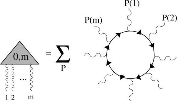
Figure 2: Initial condition for the pure boson vertices in the momentum transfer cutoff scheme. The sum is taken over the $m!$ permutations of the labels of the external legs.

The initial condition for the flow in this interaction cutoff scheme corresponds to a situation in which interaction lines are turned off while particle propagator lines are fully functional. In addition to the bare three-leg interaction vertex, the only one-line irreducible diagrams that can be drawn are closed loops of fermionic propagators. These loops have to be symmetrized with respect to the exchange of external bosonic legs in order to obtain the initial condition for the purely bosonic vertices as shown in Fig. 2. A more formal derivation of the initial condition is given in the Appendix. The result is given by

$$\Gamma_{\Lambda_{0}}[\bar{\psi},\psi,\varphi]=i(\bar{\psi},\hat{\varphi}\psi)+\frac{1}{2\beta V}\sum_{\sigma\sigma^{\prime}}[f_{0}^{-1}]^{\sigma\sigma^{\prime}}\varphi_{0\sigma}\varphi_{0\sigma^{\prime}}-\mathrm{Tr}\{\ln[\hat{1}-i\hat{G}_{0}\hat{\varphi}]\}\,,$$ (72)

where the matrix $\hat{\varphi}$ of bosonic fields is defined in analogy to Eq. (A.88) and

$$[\hat{{G}}_{0}]_{K\sigma,K^{\prime}\sigma^{\prime}}=\delta_{K,K^{\prime}}\delta_{\sigma,\sigma^{\prime}}{G}_{0,\sigma}(K)\,,\qquad{G}_{0,\sigma}(K)=[i\omega-{\xi}_{{\bm{k}}\sigma}]^{-1}\,.$$ (73)

The first two terms in Eq. (72) are nothing but the bare interaction $S_{1}$ defined in Eq. (54), whereas the last term generates the closed fermion loops.

When expanded in powers of the field $\varphi$, Eq. (72) contains linear terms. We thus need to perform the shift $\varphi_{\bar{K}\sigma}=\varphi_{\bar{K}\sigma}^{0}+\Delta\varphi_{\bar{K}\sigma}$ with $\varphi^{0}_{K\sigma}$ given in Eq. (57), yielding

$$\Gamma_{\Lambda_{0}}[\bar{\psi},\psi,\varphi]=-\mathrm{Tr}\{\ln[\hat{1}-i\hat{G}_{\varphi}\Delta\hat{\varphi}]\}+\frac{1}{2\beta V}\sum_{\sigma\sigma^{\prime}}[f_{0}^{-1}]^{\sigma\sigma^{\prime}}\Delta\varphi_{0\sigma}\Delta\varphi_{0\sigma^{\prime}}-i\sum_{\sigma}\Delta\varphi_{0\sigma}\rho_{\sigma}$$

$$~{}~{}~{}~{}~{}~{}~{}~{}~{}~{}~{}~{}~{}~{}+\bar{\varphi}_{\sigma}(\bar{\psi},\psi)+i(\bar{\psi},\Delta\hat{\varphi}\psi)-\mathrm{Tr}\{\ln[\hat{G}_{0}\hat{G}_{\varphi}^{-1}]\}-\frac{\beta V}{2}\sum_{\sigma\sigma^{\prime}}f_{0}^{\sigma\sigma^{\prime}}\rho_{\sigma}\rho_{\sigma^{\prime}}\,,$$ (74)

where we have defined the shifted bare Green function

$$\hat{G}_{\varphi}^{-1}=\hat{G}_{0}^{-1}-i\hat{\varphi}^{0}\,,$$ (75)

with the matrix elements

$$[\hat{G}_{\varphi}]_{K\sigma,K^{\prime}\sigma^{\prime}}=\delta_{K,K^{\prime}}\delta_{\sigma,\sigma^{\prime}}\tilde{G}_{0,\sigma}(K)\,,\qquad\tilde{G}_{0,\sigma}(K)=[i\omega-\tilde{\xi}_{{\bm{k}}\sigma}]^{-1}\,,$$ (76)

and $\tilde{\xi}_{{\bm{k}}\sigma}\equiv\xi_{{\bm{k}}\sigma}+\sum_{\sigma^{\prime}}f_{0}^{\sigma\sigma^{\prime}}\rho_{\sigma^{\prime}}$. From Eq. (74) the initial condition for the one-line irreducible vertices can be obtained by expanding the right-hand side in powers of $\Delta\varphi$ and by symmetrizing the resulting expressions with respect to the interchange of bosonic fields. We obtain

$$\Gamma^{(0,0)}_{\Lambda_{0}}=-\mathrm{Tr}\{\ln[\hat{G}_{0}\hat{G}_{\varphi}^{-1}]\}-\frac{\beta V}{2}\sum_{\sigma\sigma^{\prime}}f_{0}^{\sigma\sigma^{\prime}}\rho_{\sigma}\rho_{\sigma^{\prime}}$$

$$~{}~{}~{}~{}~{}=-\beta V\Big{\{}\sum_{\sigma}\int_{\bm{k}}\ln\Big{[}\frac{1+e^{-\beta\tilde{\xi}_{{\bm{k}}\sigma}}}{1+e^{-\beta\xi_{{\bm{k}}\sigma}}}\Big{]}+\frac{1}{2}\sum_{\sigma\sigma^{\prime}}f_{0}^{\sigma\sigma^{\prime}}\rho_{\sigma}\rho_{\sigma^{\prime}}\Big{\}}\,,$$ (77)

$$\Gamma^{(0,1)}_{\Lambda_{0},\sigma}=-i\left[\rho_{\sigma}-\int_{K}\tilde{G}_{0,\sigma}(K)\right]\,,$$ (78)

$$\Gamma^{(2,1)}_{\Lambda_{0}}(K+\bar{K},\sigma;K\sigma;\bar{K}\sigma)=i\,,$$ (79)

$$\Gamma^{(2,0)}_{\Lambda_{0}}(K\sigma;K\sigma)=\Sigma^{\Lambda_{0}}_{\sigma}(K)=\sum_{\sigma^{\prime}}f_{0}^{\sigma\sigma^{\prime}}\rho_{\sigma^{\prime}}\,,$$ (80)

$$\Gamma^{(0,2)}_{\Lambda_{0}}(-\bar{K}\sigma,\bar{K}\sigma)=\Pi^{\Lambda_{0}}_{\sigma,\sigma^{\prime}}(\bar{K})=[f_{0}^{-1}]^{\sigma\sigma^{\prime}}\delta_{\bar{K},0}/(\beta V)+L^{(2)}_{\sigma}(-\bar{K},\bar{K})\,,$$ (81)

and for $m\geq 2$,

$$\Gamma^{(0,m)}(\bar{K}_{1}\sigma,\dots,\bar{K}_{m}\sigma)=L_{\sigma}^{(m)}(\bar{K}_{1},\dots,\bar{K}_{m})\,.$$ (82)

All other one-line irreducible vertices vanish initially. Here, we have defined the symmetrized fermion loops as

$$L_{\sigma}^{(n)}(\bar{K}_{1},\dots,\bar{K}_{n})=\frac{i^{n}}{n}\sum_{P}\int_{K}\tilde{G}_{0,\sigma}(K)\tilde{G}_{0,\sigma}(K+\bar{K}_{P(1)})$$

$$~{}~{}~{}~{}~{}~{}~{}~{}~{}~{}~{}~{}~{}~{}~{}~{}~{}~{}~{}\cdot\dots\cdot\tilde{G}_{0,\sigma}(K+\bar{K}_{P(1)}+\ldots+\bar{K}_{P(n-1)})\,.$$ (83)

The summation is over all permutations $P$ of $\{1,\dots,n\}$. If we now demand that $\Gamma_{\Lambda_{0}}^{(0,1)}=0$, we obtain the relation

$$\rho_{\sigma}=\int_{K}\tilde{G}_{0,\sigma}(K)=\int_{\bm{k}}n_{F}(\xi_{{\bm{k}}\sigma}+\sum_{\sigma^{\prime}}f_{0}^{\sigma\sigma^{\prime}}\rho_{\sigma^{\prime}})\,,$$ (84)

which is nothing but a Hartree self-consistency condition. Hence, the initial condition in the interaction-cutoff scheme is simply the self-consistent Hartree approximation for the density. Note that Eq. (84) can also have ferromagnetic solutions with $\rho_{\uparrow}\neq\rho_{\downarrow}$.

By solving the flow equations for the purely bosonic vertices in some appropriate truncation, our approach then allows for a systematic inclusion of bosonic fluctuations around the self-consistent Hartree approximation. Since the fermionic degrees of freedom are not completely integrated out in our approach, it is in principle possible to use this solution for the bosonic vertices in the flow of vertices with external fermionic legs, e.g. to calculate approximations to the single-particle Green’s function.

5 Summary and outlook

We have presented a unified way of treating vacuum expectation values of bosonic fields in the functional renormalization group. In a simple truncation, our flow equations for the Ising model in the symmetry broken phase reduce to well known results obtained in the context of the local potential approximation. We apply our formalism to the coupled Bose-Fermi theory obtained by decoupling the electron-electron interaction in the zero-sound channel. The vacuum expectation value of the zero-frequency and zero-momentum mode of the bosonic field is in this case closely related to the fermionic density. The dependence of this vacuum expectation value at the end of the RG flow on the initial chemical potential allows us to calculate the compressibility of the system. Using a fermionic cutoff and a simple Hartree-type truncation of the flow equations, we obtain the known Fermi-liquid result for the compressibility. In the interaction-cutoff scheme, a cutoff is introduced solely in the bosonic propagator and a fermionic determinant has to be evaluated to determine the initial condition of the flow. This initial condition is then given by the self-consistent Hartree approximation and the flow equations can be used to obtain corrections to this mean-field theory.

It is straightforward to generalize the partial bosonization approach to the case where some other collective bosonic field develops a finite expectation value. For example, with the help of a Hubbard-Stratonovich transformation in the particle-particle channel, we may study fluctuation corrections to the BCS approximation for a superconductor. Note that within the interaction-cutoff scheme, the self-consistent BCS approximation should emerge as the initial condition for the coupled Fermi-Bose theory, in analogy to Eq. (84). This should be compared with the purely fermionic functional RG approach to symmetry breaking developed by Salmhofer and coauthors [6], where the BCS self-consistency condition is only generated in the limit $\Lambda\rightarrow 0$ by the RG flow starting from an infinitesimal symmetry breaking perturbation.

The truncation scheme used in Sec. 3 to study symmetry breaking in the classical Ising model can be applied to any bosonic sector of quantum systems involving both bosons and fermions. Such a procedure, which is equivalent to a truncated local potential approximation, might be a convenient starting point to study the feedback between bosonic fluctuations on the fermionic single-particle excitations.

Finally, it should be mentioned that an alternative functional RG approach, which also seems to be convenient to study spontaneous symmetry breaking, has recently been developed by Dupuis [17]. His approach is based on the functional RG flow of the generating functional of the two-particle irreducible vertex functions. Note that in fermionic language the one-line irreducible vertex functions introduced in our partial bosonization approach are only partially two-particle irreducible in the sense that two-particle irreducible diagrams singled out by the Hubbard-Stratonovich field are eliminated in favour of a collective bosonic field.

We appreciate useful discussions with N. Hasselmann, L. Bartosch and S. Ledowski. This work was partially supported by the DFG via the Forschergruppe FOR 412.

Appendix: Initial condition in the interaction-cutoff scheme

A more formal route to the initial condition (72) for $\Gamma$ in the interaction-cutoff scheme uses an additional generating functional for partially amputated-connected Green’s functions for which external interaction lines are amputated [18],

$$e^{\mathcal{G}_{\rm pac}[\bar{\jmath},j,J]}=\frac{1}{\mathcal{Z}_{0}}\int D[\bar{\psi},\psi,\varphi]e^{-S_{0}[\bar{\psi},\psi]-S_{0}[\varphi]-S_{1}[\bar{\psi},\psi,\varphi+J]+(\bar{\jmath},\psi)+(\bar{\psi},j)}\,.$$ (A.85)

By elementary manipulation of the functional integral, we can show

$$e^{\mathcal{G}_{\rm pac}[\bar{\jmath},j,J]}=e^{\frac{1}{2}\left(\frac{\delta}{\delta J},\hat{F}_{0}\frac{\delta}{\delta J}\right)}\frac{1}{\mathcal{Z}_{\psi}}\int D[\bar{\psi},\psi]e^{-S_{0}[\bar{\psi},\psi]-S_{1}[\bar{\psi},\psi,J]+(\bar{\jmath},\psi)+(\bar{\psi},j)}\,.$$ (A.86)

Here, $[\hat{F}_{0}]_{\bar{K}\sigma,\bar{K}^{\prime}\sigma^{\prime}}=\delta_{\bar{K}+\bar{K}^{\prime},0}F_{0,\sigma\sigma^{\prime}}(\bar{K}^{\prime})$ is the matrix of the bare interaction, and $\mathcal{Z}_{\psi}=\int D[\bar{\psi},\psi]e^{-S_{0}[\bar{\psi},\psi]}$ is the partition function for non-interacting particles. For the initial condition of the flow, we have $f\to 0$. This limit can readily be taken in Eq. (A.86). The remaining functional integral is Gaussian and yields

$$\mathcal{G}_{\rm pac}^{f\to 0}[\bar{\jmath},j,J]=\mathrm{Tr}\{\ln[\hat{1}-i\hat{G}_{0}\hat{J}]\}-(\bar{\jmath},[\hat{1}-i\hat{G}_{0}\hat{J}]^{-1}\hat{G}_{0}j)\,,$$ (A.87)

where we use a matrix $\hat{J}$ of bosonic sources containing the matrix elements

$$[\hat{J}]_{K\sigma,K^{\prime}\sigma^{\prime}}=\delta_{\sigma\sigma^{\prime}}J_{K-K^{\prime},\sigma}\,.$$ (A.88)

The first term in Eq. (A.87) generates the closed loops of fermion propagators in Fig. 2 when expanded in powers of the bosonic sources. The second term generates diagrams that contain a continuous fermionic path linking two external fermionic legs. An arbitrary number of external bosonic legs are then directly attached to this line. The latter diagrams are not one-line irreducible and will cancel in the expression for $\Gamma$. However, before we can perform the Legendre transformation, we first need a relation between $\mathcal{G}_{\rm pac}$ and the generating functional $\mathcal{G}_{c}$ for connected Green’s functions. This is achieved by a shift $\varphi\to\varphi-J$ in the integration variables in Eq. (A.85) and yields

$$\mathcal{G}_{c}[\bar{\jmath},j,J]=S_{0}[\tilde{J}]+\mathcal{G}_{\rm pac}[\bar{\jmath},j,\tilde{J}]\,,$$ (A.89)

where we have defined $\tilde{J}=\hat{F}_{0}J$. The classical field $\varphi$ is then given by

$$\varphi=\frac{\delta\mathcal{G}_{c}}{\delta J}=\tilde{J}+\hat{F}_{0}\frac{\delta\mathcal{G}_{\rm pac}}{\delta\tilde{J}}[\bar{\jmath},j,\tilde{J}]\stackrel{{\scriptstyle f\to 0}}{{=}}\tilde{J}\,.$$ (A.90)

In the limit of a vanishing interaction the classical field $\varphi$ thus becomes identical to the source field $\tilde{J}$. Since $\mathcal{G}_{\mathrm{pac}}^{f\to 0}$ is quadratic in the fermionic sources, the inversion necessary to obtain the sources $\bar{\jmath}$ and $j$ as a function of the classical fields involves just a matrix inversion. The remaining Legendre transformation can then be explicitly performed and we obtain Eq. (72).

References

• [1] F. Schütz, L. Bartosch, and P. Kopietz, Phys. Rev. B 72, 035107 (2005).
• [2] J. A. Hertz, Phys. Rev. B 14, 1165 (1976).
• [3] C. Wetterich, Phys. Lett. B 301, 90 (1993).
• [4] T. R. Morris, Int. J. Mod. Phys. A 9, 2411 (1994).
• [5] T. Baier, E. Bick, and C. Wetterich, Phys. Rev. B 70, 125111 (2004).
• [6] M. Salmhofer, C. Honerkamp, W. Metzner, and O. Lauscher, Prog. Theor. Phys. 112, 943 (2004).
• [7] C. Honerkamp and M. Salmhofer, Prog. Theor. Phys. 113, 1145 (2005).
• [8] R. Gersch, C. Honerkamp, D. Rohe, and W. Metzner, Eur. Phys. J. B 48, 349 (2005).
• [9] J. Berges, N. Tetradis, and C. Wetterich, Phys. Rep. 363, 223 (2002).
• [10] A. Parola, D. Pini, and L. Reatto, Phys. Rev. E 48, 3321 (1993).
• [11] A. Bonanno and G. Lacagnina, Nucl. Phys. B 693, 36 (2004).
• [12] T. Busche, L. Bartosch, and P. Kopietz, J. Phys.: Cond. Mat. 14, 8513 (2002).
• [13] S. Ledowski, N. Hasselmann, and P. Kopietz, Phys. Rev. A 69, 061601(R) (2004); N. Hasselmann, S. Ledowski, and P. Kopietz, Phys. Rev. A 70, 063621 (2004).
• [14] P. Kopietz and T. Busche, Phys. Rev. B 64, 155101 (2001); S. Ledowski, P. Kopietz, and A. Ferraz, Phys. Rev. B 71, 235106 (2005).
• [15] R. Shankar, Rev. Mod. Phys. 66, 129 (1994).
• [16] See, for example, D. Pines and P. Nozières, The Theory of Quantum Liquids, Volume I, (Addison-Wesley Advanced Book Classics, Redwood City, Ca, 1989).
• [17] N. Dupuis, Eur. Phys. J. B 48, 319 (2005).
• [18] F. Schütz, Ph. D. thesis, Universität Frankfurt (2005), URN: urn:nbn:de:hebis:30-16018, URL: http://publikationen.ub.uni-frankfurt.de/volltexte/2005/1601/.