Coupled logistic maps and non-linear differential equations

Abstract

We study the continuum space-time limit of a periodic one dimensional array of deterministic logistic maps coupled diffusively. First, we analyse this system in connection with a stochastic one dimensional Kardar-Parisi-Zhang (KPZ) equation for confined surface fluctuations. We compare the large-scale and long-time behaviour of space-time correlations in both systems. The dynamic structure factor of the coupled map lattice (CML) of logistic units in its deep chaotic regime and the usual $d=1$ KPZ equation have a similar temporal stretched exponential relaxation. Conversely, the spatial scaling and, in particular, the size dependence are very different due to the intrinsic confinement of the fluctuations in the CML. We discuss the range of values of the non-linear parameter in the logistic map elements and the elastic coefficient coupling neighbours on the ring for which the connection with the KPZ-like equation holds. In the same spirit, we derive a continuum partial differential equation governing the evolution of the Lyapunov vector and we confirm that its space-time behaviour becomes the one of KPZ. Finally, we briefly discuss the interpretation of the continuum limit of the CML as a Fisher-Kolmogorov-Petrovsky-Piscounov (FKPP) non-linear diffusion equation with an additional KPZ non-linearity and the possibility of developing travelling wave configurations.

1 Introduction

Extended dynamical systems can be modelled with infinite dimensional non-linear partial differential equations but also with coupled map lattices (CMLs). The relation between the two and, in particular, their behaviour in the spatio-temporal chaotic regime is a subject of great interest [1].

Whether local chaos can be modelled by stochastic noise is a very deep question that has been addressed from different angles and with a variety of analytical and numerical approaches. Back in the 40’s Von Neumann and Ulam proposed to use the logistic map in its chaotic domain as a pseudo random number generator [2]. Except for a set of initial values of measure zero, the iterates of the logistic map are distributed according to $p(x)=[\pi^{2}\,x(1-x)]^{-1/2}$ and the sequence $T^{-1}(x)$ with $T(x)=\sin^{2}(\pi/2x)$ is equidistributed within the unit interval $[0,1]$. However, it was later realized that the time series thus generated has a number of defects, such as time-correlations and a trivial first return-map; the logistic map was subsequently neglected as a pseudo-random number generator [3, 4].

The question above was later revisited in the context of extended dynamical systems modelled with either discrete models or continuous partial differential equations. CMLs with short-range spatial interactions and chaotic dynamics of the independent units develop collective behaviour and long-range order in finite regions of the phase diagram characterised by the strength of the non-linearity and the coupling between the dynamic units [5]. Some statistical mechanics notions were shown to be useful to describe their spatiotemporal behaviour [6]-[13].

On the continuum side, in [14]-[21] the authors compared the deterministic, driven by inherent instabilities, Kuramoto-Sivashinsky (KS) partial differential equation equation [22, 23] to the stochastic Kardar-Parisi-Zhang (KPZ) partial differential equation [24]-[26] for surface growth. A careful study of the scaling properties of the solution of both equations showed that they are identical in $d=1$ but differ in $d\geq 2$ [16, 17], a result confirmed numerically in [19].

In this paper we investigate the spatio-temporal behaviour of a one dimensional ring of coupled logistic maps by taking a formal continuum space-time limit. First, we identify two non-linear terms as leading to effective noise and confinement and we argue that the CML has a long wave-length, long time behaviour that is very similar to the one of a modified KPZ equation describing surface fluctuations in a confining potential. Second, we revisit the equation for the evolution of the Lyapunov vector using similar arguments [27]. Finally, we reckon that the resulting partial differential equation is an extension of the Fisher-Kolmogorov-Petrovsky-Piscounov (FKPP) [28] non-linear diffusion equation with an additional KPZ-like non-linearity and we exhibit some travelling wave solutions.

The article is organized as follows. In Section 2 we recall the definition of the logistic map and the CML model we study. In Section 3 we review the partial differential equations we are concerned with. We first describe the KS and KPZ partial differential equations and we recall the connection between them in $d=1$. We then present the FKPP equation and some properties of its travelling wave solutions. In these first sections we also set the notation and we explain our goal. In Section 4 we define the continuum limit and we discuss each term in the resulting partial differential equation. In Section 5 we present the results of the numerical integration of the CML. We test the ‘noise’ term, we confront the behaviour of several observables to the corresponding ones in KPZ one dimensional growth, and we discuss the behaviour of the Lyapunov vector. Section 6 is devoted to a brief discussion of the travelling wave solutions. Finally, in Section 7 we present our conclusions and we discuss several proposals for future research.

2 Coupled logistic maps

2.1 The logistic map

The logistic map is a non-linear evolution equation acting on a continuous variable $x$ taking values in the unit interval $[0,1]$. The evolution is defined by iterations over discrete time, $n=0,1,\dots$:

$$x_{n}=f(x_{n-1})\equiv r\,x_{n-1}(1-x_{n-1})\;,$$ (1)

with the parameter $r$ taking values $0<r\leq 4$. The time series has very different behaviour depending on the value of $r$. For $0\leq r<1$ the iteration approaches the fixed point $x^{*}=0$. For $1\leq r<3$ the asymptotic solution takes the finite value $x^{*}(r)=1-1/r$ for almost any initial condition. Beyond $r=3$ the asymptotic solution bifurcates, $x_{n}$ oscillates between two values $x_{1}^{*}$ and $x_{2}^{*}$, and the solution has period $2$. Increasing the value of $r$ other bifurcations appear at sharp values, i.e. further period doubling takes place. Very complex dynamic behaviour arises from the relatively simple non-linear map (1) in the range $r\in[3.57,1]$: the map has bands of chaotic behaviour, i.e. different initial conditions exponentially diverge, intertwined with windows of periodic behaviour. Surprisingly enough, some exact solutions are known for special values of $r$ [31]. For example $x_{n}=\sin^{2}(\theta\pi 2^{n})$ with $k$ integer and $\theta$ determined by the initial condition through $x_{0}=\sin^{2}(\theta\pi)$ is a solution for $r=4$  [32].

2.2 Coupled map lattices

Coupled map lattices (CMLs) [5] are discrete arrays of scalar variables taking continuous values, typically in the unit interval, that evolve over discrete time according to a dynamic rule. They are generalisations of cellular automata for which the variables take only discrete values. Kaneko introduced them as phenomenological models to describe media with high energy pumping but they may also arise as discrete versions of partial differential equations.

A typical realization of the evolution of a single independent unit is given by the logistic map (1). One usually uses models in one or two space dimensions with periodic boundary conditions (a ring or a torus). A Laplacian coupling among nearest-neighbours on the lattice is usually chosen as it is motivated by the intent to model fluid mechanics in a simpler manner. In $d=1$, and labelling with $i=1,\dots,N$ the sites on the ring, the coupled map model takes the form

$$x^{i}_{n}=f(x_{n-1}^{i})+\frac{\nu}{2}\,[\,f(x_{n-1}^{i-1})-2f(x_{n-1}^{i})+f(x_{n-1}^{i+1})\,]$$ (2)

with $x_{n}^{i+N}=x_{n}^{i}$ for all $n$ with $N$ the number of elements on the ring. The initial condition is usually chosen to be random and thus taken from the uniform distribution on the interval $[0,1]$ independently on each site. $\nu$ is the coupling strength between the nodes and plays the role of a viscosity.

Numerical simulations showed that CMLs exhibit a large variety of space-time patterns: kink-antikink configurations, space-time periodic structures, wavelike patterns or spatially periodic structures with steady, periodic or chaotic dynamics, space-time intermittent and spatio-temporal chaos have been found for different values of the parameters ($r$ and $\nu$). A detailed description of the phase diagram is given in [5]. In a nutshell, the dynamics is characterised by a competition between the diffusion term, that tends to produce an homogeneous behaviour in space, and the chaotic motion of each unit, that favours spatial inhomogeneous behaviour due to the high sensitivity to the initial conditions.

3 Partial differential equations

The $d=1$ Kuramoto-Sivashinsky (KS) equation was introduced by Kuramoto to study local phase turbulence in cyclic chemical reactions [22]. A $d=2$ extension of it was later used by Sivashinsky to study the propagation of flame fronts in mild combustion [23]. In $d=1$ it reads

$$\frac{\partial h}{\partial t}=-\kappa h-\frac{\partial^{2}h}{\partial x^{2}}-\frac{\partial^{4}h}{\partial x^{4}}-h\frac{\partial h}{\partial x}$$ (3)

with $h=h(x,t)$ a real function and $\kappa$ a real parameter. Similar pattern formation to the one developed in CMLs has been observed in the numerical solutions of the KS partial differential equation [33].

The Kardar-Parisi-Zhang (KPZ) equation was proposed as a non-linear model that describes surface growth [24]. If $h(x,t)$ is the height of a surface on a substrate point $x$ at time $t$, the equation reads

$$\frac{\partial h}{\partial t}=\nu\frac{\partial^{2}h}{\partial x^{2}}+\frac{\lambda}{2}\left(\frac{\partial h}{\partial x}\right)^{2}+\eta(x,t)$$ (4)

with $\eta(x,t)$ a Gaussian white noise with zero mean and correlation given by

$$\langle\,\eta(x,t)\eta(x^{\prime},t^{\prime})\,\rangle=D\,\delta(x-x^{\prime})\,\delta(t-t^{\prime})\;.$$ (5)

The variable $dh/dx$ satisfies a noisy Burgers equation [25]. (For a discussion of the properties of these equations see ref. [26].)

Using a dynamic renormalisation group calculation, Yakhot suggested that the elimination of large wave-vector modes generates a random ‘stirring force’ with zero mean and average $\langle\,f_{i}(\vec{k},\omega)f_{j}(\vec{k}^{\prime},\omega^{\prime})\,\rangle=k_{i}k_{j}\,\delta(\vec{k}+\vec{k}^{\prime})\,\delta(\omega+\omega^{\prime})$. The average $\langle\dots\rangle$ represents a time-average in the stationary state. Simplifying further the propagator in the $\vec{k}\to 0$ limit, he argued that in the large scale and long time limit, $\vec{k}\to 0$ and $\omega\to 0$, the KS equation becomes the random-force-driven Burgers equation or, under a change of variables, the KPZ equation (with positive viscosity in $d=1$ and negative viscosity in $d\geq 2$) [14].

Next came a number of papers in which L’vov, Procaccia et al [15]-[17] studied this problem in more detail. They showed that for both equations the field-field correlation in Fourier space, $n(\vec{k},\omega)$, defined from

$$\langle\,h(\vec{k},\omega)h^{*}(\vec{k}^{\prime},\omega^{\prime})\,\rangle=n(\vec{k},\omega)\,\delta(\vec{k}-\vec{k}^{\prime})\,\delta(\omega-\omega^{\prime})\;,$$ (6)

has a scale invariant form

$$n(\vec{k},\omega)=\frac{n(\vec{k})}{\nu k^{z}}\;f\left(\frac{\omega}{\nu k^{z}}\right)\;,\qquad n(\vec{k})=\int_{\omega}n(\vec{k},\omega)=\frac{n}{k^{2\alpha+d}}\;,$$ (7)

with the ‘roughness exponent’ $\alpha$ and the ‘dynamic exponent’ $z$ being equal to $1/2$ and $3/2$ in $d=1$, respectively [15]. Under the assumption that a scale invariant solution of the form (7) also exists in $d>1$, L’vov and Procaccia [16] argued that the scaling solutions for the two models bifurcate in $d=2$; that is to say, the exponents $z$ and $\alpha$ are not the same in all dimensions and hence the two equations do not belong to the same universality class. Further evidence for the breakdown of the relation between KS and the strong coupling phase of KPZ in $d\geq 2$ appeared in [17].

It has been difficult to verify the coincidence of the scaling solution to the KS and KPZ equations in $d=1$ by solving the KS equation numerically and comparing to the prediction $z=3/2$. The reason for this difficulty is the existence of a very long crossover regime [18]. A careful numerical study appeared in [19] where large scale simulations were confronted to the predictions for the crossover behaviour obtained from the analysis of the KPZ equation.

The Fisher-Kolmogorov-Petrovsky-Piscounov (FKPP) non-linear diffusion equation determines the evolution of the concentration of some chemical species or individuals, $0\leq h\leq 1$, on a one dimensional space and reads

$$\frac{\partial h}{\partial t}=\nu\frac{\partial^{2}h}{\partial x^{2}}+f(h)\;,$$ (8)

with $f(h)$ a non-linear term, typically of the form $f(h)=k_{1}h-k_{2}h^{2}$ with $k_{1}>0$ and $k_{2}>0$. The FKPP equation has travelling wave solutions [30]

$$h(x,t)=F(x-vt)$$ (9)

that represent the invasion of the stable phase $h(-\infty,0)=k_{1}/k_{2}$ in the unstable phase $h(\infty,0)=0$ and travel with velocity $v\geq 2\sqrt{k_{1}}$. Which velocity is selected depends on the initial condition. In many cases, if the initial front is “sufficiently steep”, i.e. $F(y)$ decays faster than $e^{-\gamma_{min}y}$ for $y\to\infty$  the front advances asymptotically with the minimal velocity $v_{min}$. These are called “pulled fronts”: the leading edge of the front pulls the interface through growing linear perturbations about the unstable $h=0$ value. In these cases, the velocity approaches $v_{min}$ as a power law

$$v(t)=v_{min}-\frac{3}{2\gamma_{min}t}+{\cal O}(t^{-3/2})\;.$$ (10)

In “pushed fronts” instead it is the non-linear growth in the region behind the leading edge that pushes the interface and the asymptotic velocity is larger than $v_{min}$.

4 The continuum limit of the CMLs

In this Section we define the continuum limit and we briefly discuss each term in the resulting partial differential equation by making an explicit comparison to the ones in the KPZ equation (4) and the FKPP equation (8).

4.1 The continuum limit

The main idea is to take the continuum limit of the CML using the following discretisation of time and space derivatives:

$$\frac{\partial h}{\partial t}\;\;\; \leftrightarrow \;\;\;\frac{h_{n+1}^{i}-h_{n}^{i}}{\delta t}\;,$$ (11)

$$\frac{\partial h}{\partial x}\;\;\; \leftrightarrow \;\;\;\frac{h^{i+1}_{n}-h_{n}^{i}}{\delta x}\;,$$ (12)

$$\frac{\partial^{2}h}{\partial x^{2}}\;\;\; \leftrightarrow \;\;\;\frac{h_{n}^{i+1}-2h_{n}^{i}+h_{n}^{i-1}}{(\delta x)^{2}}\;,$$ (13)

$$\frac{\partial^{4}h}{\partial x^{4}}\;\;\; \leftrightarrow \;\;\;\frac{h_{n}^{i+2}-4h_{n}^{i+1}+6h_{n}^{i}-4h_{n}^{i-1}+h_{n}^{i-2}}{(\delta x)^{4}}\;,$$ (14)

with $\delta t$ the time-step and $\delta x$ the lattice spacing equal one in our system of units. The CML of logistic elements then becomes

$$\frac{\partial h}{\partial t} = \frac{\nu r}{2}(1-2h)\;\frac{\partial^{2}h}{\partial x^{2}}-\nu r\left(\frac{\partial h}{\partial x}\right)^{2}+(r-1)h-rh^{2}\;,$$ (15)

where we called $x$ the coordinate ($i\delta x\to x$), $t$ the time $(n\delta t\to t$), and $h$ the field [$x_{n}^{i}\to h(x,t)=h$].

4.2 Relation with KPZ

Comparing to eq. (4) one notices that:

1. By definition the field $h$ is bounded and takes values in the unit interval. Thus, the resulting equation should have an effective confining potential that limits the field to a finite range.

2. The elastic term is here multiplied by a field-dependent viscosity

   $$\nu(h)\equiv\frac{\nu r}{2}(1-2h)\;.$$ (16)

3. The second, non-linear term is of the form of the one in the KPZ equation with a negative coupling

   $$\lambda\equiv-\nu r\;.$$ (17)

4. The last two terms read

   $$\eta(x,t)\equiv(r-1)h(x,t)-rh^{2}(x,t)\;.$$ (18)

   We notice that these terms are not present in the KPZ equation. In order to compare to the latter we shall argue that they have a double identity: on the one hand $\eta$ behaves roughly as a short-range correlated noise in space and time; on the other hand it can be interpreted as a force derived from a confining potential

   $$\eta=-\frac{\partial V(h)}{\partial h}\;,\qquad\qquad V(h)=-\frac{(r-1)}{2}h^{2}+\frac{r}{3}h^{3}\;.$$ (19)

In the next subsections we briefly discuss the elastic and non-linear terms. The analysis of $\eta$ is more delicate and we postpone it to the next section where we present the results of the numerical integration of the CML.

4.2.1 The elastic term.

The fact that the elastic term is multiplied by a field-dependent viscosity needs a careful inspection.

First, $\nu(h)$ is negative for $h<1/2$ which implies an instability in the hydrodynamic limit. The same feature appears in the KS equation [eq. (3)]. It was shown that this instability taps the system and so creates an effective ‘noise’ leading to the mapping of the KS equation onto a similar equation with a noise term and a renormalised positive viscosity coefficient [14, 15] (see the discussion in Sect. 3). With respect to this ‘noise creation’ feature, it is also very important to have a confining potential which restraints the instabilities caused by the negative values of $\nu(h)$. Together they create the effective noise. Therefore, the fact that we may get negative values for the viscosity actually supports our line of argumentation, i.e. that of relating a deterministic model to a stochastic one.

Second, if $h$ remains bounded between, say, 0 and 1 the ‘bare’ viscosity takes values on the finite interval $[-\frac{\nu r}{2},\frac{\nu r}{2}]$. However, as is well known, in the KPZ system the viscosity coefficient is renormalised by the nonlinear term (put in simple words, the nonlinear term has a smoothing effect) so that the large-scale viscosity that the system experiences is not only determined by the bare value. Thus, we also expect the field-dependent bare viscosity to be renormalised at large scales and thus its precise value not to be very important.

4.2.2 The non-linear term.

It is well-known that the sign of the coupling constant is not important in the KPZ equation. The reason is that an inversion of the sign of $\lambda$ just corresponds to describing the evolution of the mirror image of the original surface (i.e. a description of $-h(x,t)$, see e.g. [26]). Actually, when mapping the noisy Burgers equation onto the KPZ equation the resulting coupling constant is negative, namely $\lambda=-1$.

4.3 Relation with FKPP

Comparing to eq. (8) one realizes that

1. The field $h$ is bounded as in FKPP.

2. The viscosity is now field dependent and may take negative values.

3. There is a KPZ-like non-linearity, not present in the FKPP equation.

4. The last two terms are identical to the ones in the FKPP equation with $k_{1}=r-1$ and $k_{2}=r$.

The similarity with the FKPP equation suggests to search for travelling wave solutions in the CML and study their properties (velocity, etc.) as done for the FKPP equation [30]. We shall come back to this issue in Sect. 6.

5 Numerical tests in the context of surface growth

We integrated numerically the CML of logistic units with up to $N=1024$ sites and periodic boundary conditions. All units were updated in parallel. We used floating point precision $10^{-16}$. Unless otherwise stated we chose independent random initial conditions for each map taken from the unit interval with flat probability. Since finite-size effects seem to be negligible for systems larger than approximately $32$ sites [45], we do not discuss smaller systems, nor do we make a systematic study of finite-size scaling. In particular, we discuss the choice of parameters in Sect. 5.1, we study the statistical properties of the $\eta$ term in Sect. 5.2, we compare the spatial and temporal behaviour of correlation functions in the CML and KPZ growth in Sect. 5.3, and we analyse the Lyapunov vector in Sect. 5.4.

5.1 Choice of parameters

The panels in Fig. 1 present the space-time plot of a coarse-grained variable obtained by transforming the continuous variable $x_{n}^{i}$ into a bi-valued Ising-like one $s_{n}^{i}=\mbox{sign}(x_{n}^{i}-x^{*})$ for several values of the non-linear parameter $r$ and the coupling strength $\nu=0.4$. We draw time on the horizontal axis and space on the vertical one. Every $50$ time step is plotted; if $x_{n}^{i}$ is larger than $x^{*}=1-1/r$ (the unstable fixed point of a single logistic map) the corresponding pixel is painted black; otherwise it is left white. This analysis allows us to identify different regions of phase space [5] in which we can study the connection with the KPZ equation. In this work we focus on $\nu=0.4$ and $r=4$, i.e. deep in the chaotic regime. We briefly mention at the end of this Section the behaviour found for other values of $\nu$ and $r$.

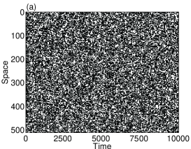
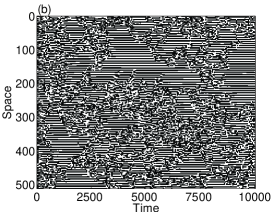
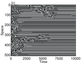
Figure 1: Space-time plots of the coarse-grained variable $s_{n}^{i}=\mbox{sign}(x_{n}^{i}-x^{*})$ for (a) $r=4$, (b) $r=3.82$, and (c) $r=3.8$.

5.2 Analysis of $\eta(x,t)$

5.2.1 The noisy aspect.

Before studying the properties of $\eta$ in the CML let us recall some properties of this quantity in the single map. Choosing the parameter $r$ to be $r=4$, i.e. well in the chaotic regime, we obtain the histogram of $x_{n}$ over a time window of length $T=10^{6}$ shown in Fig. 2(a). The figure demonstrates that the numerical precision chosen is good enough for our purposes since the data are rather well described by the analytic prediction for the probability distribution function (PDF)

$$p(x)=\frac{1}{\pi\sqrt{x(1-x)}}\;.$$ (20)

The divergence of the peaks at $x=0$ and $x=1$ is however suppressed due to the floating point precision of the numerical data. The histogram is symmetric around $x=1/2$ and, consequently, the mean is given by $\langle\,x\,\rangle\equiv T^{-1}\sum_{n-1}^{T}x_{n}=1/2$.

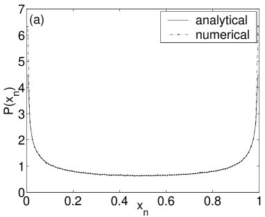
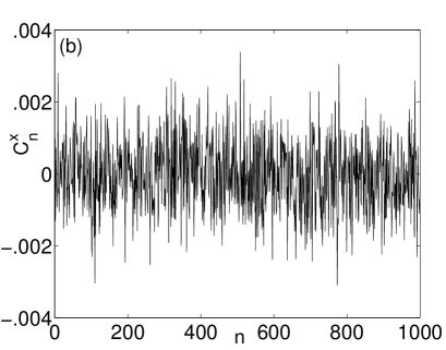
Figure 2: (a) The PDF of a single map $x_{n}$, and (b) the evolution of its autocorrelation function $C_{n}^{x}$ defined in eq. (21).

In Fig. 2(b) we show the connected correlation over time,

$$C_{n}^{x}\equiv\langle\,\Delta x_{k+n}\Delta x_{k}\,\rangle=\frac{1}{T-n}\sum_{k=0}^{T-n}\Delta x_{k+n}\Delta x_{k}\;,$$ (21)

for a single run using a randomly chosen seed. $\Delta x_{k}\equiv x_{k}-1/2$ and the average is taken over all pairs of data obtained with a time delay $n$ on a single run of length $T=10^{6}$. No correlations can be identified from this plot though we know, however, that some time-structure might be present [35] (see, e.g. the return map in Fig. 8).

We now turn to the study of

$$\eta_{n}\equiv(r-1)x_{n}-rx_{n}^{2}\;.$$ (22)

By definition, $\eta_{n}$ takes values in the interval $[-1,(r-1)^{2}/(4r)]$ that for $r=4$ becomes $[-1,9/16]$. In Fig. 3(a) we show the histogram of $\eta_{n}$ corresponding to the same data shown in Fig. 2. Actually, using the PDF of $x_{n}$ in eq. (20) we derive the PDF of $\eta_{n}$ that is given by

$$p\left(\eta\right) = \frac{1}{{2\pi\sqrt{\frac{3}{4}-\sqrt{\frac{9}{{16}}-\eta}}\sqrt{\frac{5}{4}+\sqrt{\frac{9}{{16}}-\eta}}\sqrt{\frac{9}{{16}}-\eta}}}\;\theta\left(\eta\right)$$ (23)

$$+\frac{1}{{2\pi\sqrt{\frac{3}{4}+\sqrt{\frac{9}{{16}}-\eta}}\sqrt{\frac{5}{4}-\sqrt{\frac{9}{{16}}-\eta}}\sqrt{\frac{9}{{16}}-\eta}}}\;.$$

where $\theta(\eta)$ is the Heaviside (step) function. The numerical histogram is well-described by this analytic function with the proviso that the divergences are replaced by the peaks in the figure. Using this expression for $p(\eta)$ one finds that the average of $\eta$ vanishes

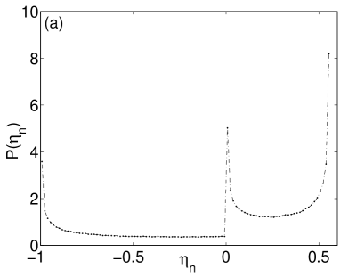
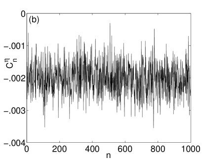
Figure 3: (a) The PDF of the ‘noise’ term in a single map $\eta_{n}$. (b) The evolution of its connected autocorrelation function, $C_{n}^{\eta}$, over time.

$$\langle\,\eta\,\rangle=(r-1)\langle\,x\,\rangle-r\langle\,x^{2}\,\rangle=3\times\frac{1}{2}-4\times\frac{3}{8}=0\;.$$ (24)

A vanishing mean is recovered by computing the average numerically. Similarly we get

$$\mbox{Skewness}=\frac{\langle\eta^{3}\rangle}{\langle\eta^{2}\rangle^{3/2}}=-\frac{3}{4}\;,\qquad\mbox{Kurtosis}=\frac{\langle\eta^{4}\rangle}{\langle\eta^{2}\rangle^{2}}=\frac{9}{4}\;.$$ (25)

The time dependence of the connected autocorrelations, $C^{\eta}_{n}\equiv\langle\,\Delta\eta_{k+n}\Delta\eta_{k}\,\rangle\equiv{(T-n)}^{-1}\sum_{k=0}\Delta\eta_{k+n}\Delta\eta_{k}=$${(T-n)}^{-1}\sum_{k=0}\eta_{k+n}\eta_{k}$, are shown in Fig. 3(b) and again no obvious structure is observed.

Next, we study the noise term in the CML. In Fig. 4(a) we show a representative histogram of the individual units $x_{n}^{i}$. This PDF is clearly smoother than the one of the independent map shown in Fig. 2(a). For the rather high value of the coupling strength used, $\nu=0.4$, all units behave statistically in the same way. The average is $\langle\,x\,\rangle\approx 0.67$. In Fig. 4(b) we show a representative histogram of the individual noise terms. Apart from a high peak at $\eta\approx 0.5625$ (which is just the maximum allowed value $9/16$ within our numerical accuracy) the plot is almost flat. The average is $\langle\,\eta\,\rangle\approx 0$.

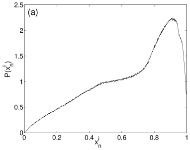
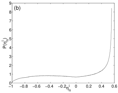
Figure 4: The PDF of (a) a typical map $x^{i}_{n}$ and (b) a typical noise term in the fully chaotic regime ($r=4$).

Since the connected correlation over time of a single map is rather noisy we prefer to show its average over all sites in the system. More precisely, in Fig. 5 we show the time decay of

$$[\,C^{\eta}_{n}\,]\equiv[\langle\,\Delta\eta_{k+n}\,\Delta\eta_{k}\,\rangle]=\frac{1}{N}\sum_{i=1}^{N}\left(\frac{1}{T-n}\sum_{k=0}^{T-n}\eta^{i}_{k}\,\eta^{i}_{k+n}\right)\;,$$ (26)

where we used $\langle\,\eta_{k}\,\rangle\approx 0$. Here and in what follows we use square brackets to denote an average over space. We chose the scaling with $n^{2/3}$ of the time axis and a logarithmic scale of the vertical axis to make clear that the time-correlations decay as a stretched exponential:

$$[\,C^{\eta}_{n}\,]\approx e^{-\alpha n^{2/3}}\;.$$ (27)

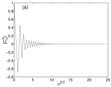
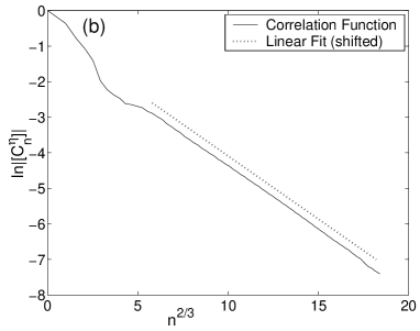
Figure 5: Decay in time of the auto-correlation of the noise on a site averaged over all sites in the sample, $[\,C_{n}^{\eta}\,]$, as a function of $n^{2/3}$ [(a) linear plot, (b) linear-logarithmic scale].

Even though we cannot exclude an additional power law dependence on time this result demonstrates that the time correlations of the noise $\eta$ are very short-ranged. Note the oscillations at short times in Fig. 5(a) that are not visible in Fig. 5(b) due to the absolute value.

We also studied the spatial correlations of $\eta$. In Fig. 6 we display the equal time correlation

$$\overline{C^{\eta}_{i}}\equiv\frac{1}{T}\sum_{k=1}^{T}\left(\frac{1}{N-i}\sum_{j=0}^{N-i}\eta^{j}_{k}\,\eta^{j+i}_{k}\right)\;.$$ (28)

Here and in what follows the overline indicates an average over time. The line is a guide-to-the-eye showing the exponential decay

$$\overline{C^{\eta}_{i}}\approx e^{-i/\xi}\;,\qquad\qquad\xi\sim 46\;,$$ (29)

defining a ‘correlation length’, $\xi$, which is finite but rather long. The oscillations can also be taken into account, but we omit their precise functional description here.

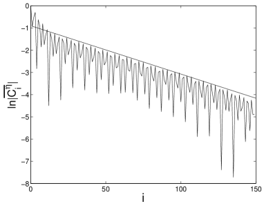
Figure 6: Decay of the equal-time spatial correlations - $\overline{C^{\eta}_{i}}$ defined in eq. (28) (in linear-logarithmic scale). The line corresponds to $e^{-i/\xi}$ with $\xi\approx 46$.

The short-range correlations in time and space shown in Figs. 5 and 6 are confirmed by an analysis of the PDFs of space and time averages of the noise itself,

$$\overline{\eta^{i}}\equiv\frac{1}{T}\sum_{n=1}^{T}\eta_{n}^{i}\;,\qquad\qquad[\,\eta_{n}\,]\equiv\frac{1}{N}\sum_{i=1}^{N}\eta_{n}^{i}\;,$$ (30)

that are quite Gaussian, as shown in Fig. 7(a) and Fig. 7(b), respectively. The data used to draw the histograms are taken from the horizontal average at fixed vertical position, and the vertical average at fixed horizontal position, respectively, of the original continuous value of $x_{n}^{i}$ that gave rise to the space-time map of Fig. 1(a).

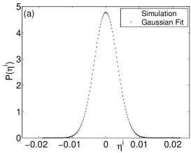
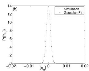
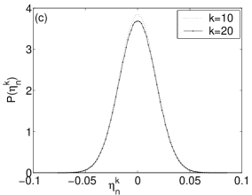
Figure 7: The PDFs of (a) $\overline{\eta^{i}}$, (b) $[\,\eta_{n}\,]$, and (c) Re$\left[\eta^{k}_{n}\right]$ for $k=10,\,20$.

One can also draw the histograms of different Fourier components $\overline{\eta^{k}}$ [the case $k=0$ actually corresponds to Fig. 7(a)] which turn out to be also Gaussian, as can be seen in Fig 7(c) where the cases $k=10$ and $k=20$ are displayed.

5.2.2 The confining aspect.

In the previous subsection we studied the statistical properties of the values taken by $\eta_{n}^{i}$ along a dynamical run. We here analyse the effect of $\eta_{n}^{i}$ as a deterministic force deriving from the potential (19).

The fact that $\eta_{n}^{i}$ is not really a perfect noise can be seen from the study of the return maps. Figure 8(a) shows the first return map, i.e. the plot of $\eta^{j}_{n+1}$ as a function of $\eta^{j}_{n}$ for many values of $n$ and a chosen site on the lattice. The information encoded in this plot is not included in the analysis of the temporal correlations.

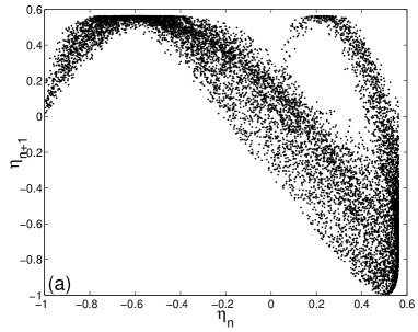
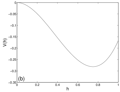
Figure 8: (a) First return map, $\eta_{n+1}^{j}$ against $\eta_{n}^{j}$, for a typical site in the fully chaotic regime ($r=4$). (b) The confining potential $V(h)$ given in eq. (19).

Even though the map is not a simple one-dimensional line, but rather occupies some non-vanishing area, it does not fill phase space. In other words, the return map is not structureless and therefore in some sense not completely chaotic/stochastic (see ref. [4]). This plot demonstrates that unpredictability (i.e. no correlations) does not imply randomness.

The bound on the original logistic map variables should translate onto a confinement of the surface fluctuations $h$. The interpretation of $\eta$ as a force deriving from the potential $V(h)$ shown in Fig. 8(b) allows one to identify this term as an important one providing the confinement of the fluctuations. For small $h$, more precisely, $h<(r-1)/r$ ($=3/4$ for $r=4$) the force is positive and it tends to increase the value of $h$. Instead, for large $h$, $h>(r-1)/r$ the force is negative and it pushes the fluctuation to take smaller values [a similar confining effect is produced in the KS equation (3) by the term $-\kappa h$].

5.2.3 The non-linear aspect.

$\eta$ has the same structure as the non-linear terms in the diffusive and otherwise linear FKPP equation. It is then clear that eq. (15) admits the same spatially uniform and constant fixed points $h=0$ and $h=(r-1)/r$. One can then expect to find travelling wave solutions when special initial conditions are chosen. We present some examples in Sect. 6 but we delay their detailed numerical study to [56].

5.3 The CML against KPZ: observables

We here translate the definition of the observables of interest in the KPZ framework to that of the CML and we confront their behaviour in the two system.

5.3.1 Confinement.

In the CML the variables are bounded and the mean-square displacement cannot be larger than $1$. In Fig. 9 we show a snapshot of a CML (a), a KPZ surface (b) and a confined KPZ surface (c). At face value these figures look different, although one can find similarities between the CML and confined KPZ surfaces. Also, these figures are very different from the KPZ surface being confined between two ‘soft’ walls [36].

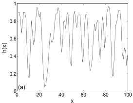
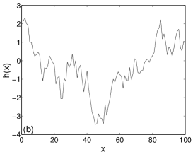
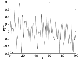
Figure 9: (a) A CML interface, (b) a KPZ interface and (c) a confined KPZ interface (with a confining potential of $-\frac{1}{20}h^{2}$).

Let us now compare the space and time dependence of these surfaces in more detail.

5.3.2 Roughness.

Stochastic surface growth from a flat initial configuration is usually characterised in terms of the mean-square displacement $w^{2}$. In a one dimensional discrete model $w^{2}$ reads

$$w_{\eta}^{2}(L,t)\equiv\frac{1}{L}\sum_{i=1}^{L}\left[h^{i}(t)-\frac{1}{L}\sum_{j=1}^{L}h^{j}(t)\right]^{2}\;.$$ (31)

The square root of the noise averaged displacement, $w(L,t)\equiv\sqrt{\langle\,w_{\eta}^{2}(L,t)\,\rangle}$ has the scaling behaviour [26]

$$w(L,t)\sim L^{\alpha}f\left(\frac{t}{L^{z}}\right)\;,\qquad f(u)\sim\left\{\begin{array}[]{ll}u^{\frac{\alpha}{z}}\;,&u\ll 1\;\;(\mbox{growth})\;,\\ {\mbox{c}onst}\;,&u\gg 1\;\;(\mbox{saturation})\;,\end{array}\right.$$ (34)

with $\alpha$ and $z$ the roughness and dynamic exponents, respectively.

Since the CML surface is necessarily bounded, if the scaling form (34) holds, $\alpha$ must be identically zero. If we wish to check $z$ numerically we need to specify the initial conditions. In the CML a flat configuration $x_{0}^{i}=x$ for all sites remains the same at all later times. In order to generate a rough configuration we need to introduce some disorder initially. This can be done in a number of ways. For example, one can analyse the motion of an initial localised bump on an otherwise flat configuration or one can add some small random noise on a flat state. In Fig. 10 we present results of a simulation of the CML, with random, though very small, initial condition and for several system sizes.

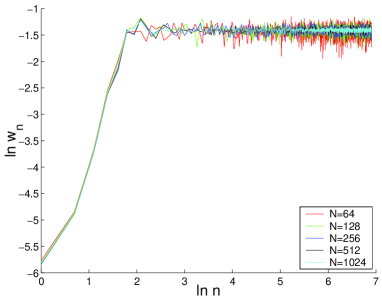
Figure 10: Roughening of a CML with small random initial conditions for various system sizes given in the key.

As can be seen in the figure, the saturation time does not depend on the size of the system, and occurs after $\sim 10$ time steps in all cases. Also, the width in the steady-state (i.e. $w_{n}$ for large $n$’s) is also independent of system size. These findings are consistent with vanishing exponents $z=0$ and $\alpha=0$ [see eq. (34)]. Actually, vanishing $\alpha$ and $z$ is also consistent with a simple scaling argument applied to the confined KPZ equation, with a confining potential of $-\frac{\kappa}{2}h^{2}$ (at this point it is worthwhile mentioning that some confined KPZ systems have been studied in the past [36] though, as far as we know, non is directly relevant here).

The non-trivial character of the PDF of mean-square displacements found in several unbounded surface growth problems [37] is completely erased by the confinement.

5.3.3 Stretched exponential relaxation.

The decay in time of the field-field correlations is still non-trivial in this system and very similar to the one found for the (usual and unbounded) KPZ equation. In Fig. 11 we show the space averaged, time correlation of the field $[\,\langle\,h_{m+n}\,h_{m}\,\rangle]$.

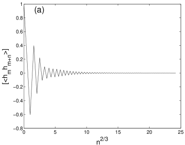
Figure 11: The correlation function $[\,\langle\,h_{m+n}\,h_{m}\,\rangle]$ as a function of $n^{2/3}$ [(a) linear plot, (b) linear-logarithmic scale).

The linear dependence in the linear-logarithmic scale used in panel (b) indicates the stretched exponential decay

$$C_{n}^{h}(t)\approx e^{-n^{\zeta}}\;,\qquad\mbox{with}\qquad\zeta=2/3\;,$$ (35)

The panel (a) shows that the decay occurs in an oscillatory way.

A stretched exponential relaxation of the dynamical structure factor in the $d=1$-KPZ growth,

$$C(k,t)\equiv\langle\,h(k,t)h^{*}(k,0)\,\rangle\sim Ae^{-Bkt^{1/z}}$$ (36)

with $z$ the dynamic exponent was found by solving the KPZ equation within the mode-coupling approximation [38], with a self-consistent expansion [39] and with a direct numerical integration in $d=1$ [40]. An oscillatory superimposed dependence on time was obtained numerically [38, 40] and can also be obtained analytically from the self-consistent expansion [41]. Some doubt on this result was shed by the solution to a polynuclear growth problem that is in the same universality class as $d=1$ KPZ [42] with a dynamic structure factor with a simple exponential decay. This discrepancy may be due to the fact that defining universality classes out of equilibrium might tricky: some models may share the static exponents but differ in their overall dynamical behaviour [40].

We thus found that the dynamic structure factor of the CML of logistic units in their deep chaotic regime ($r=4$) and the $d=1$ KPZ equation have the same stretched exponential relaxation. Surprisingly enough, the dynamic exponent $z=3/2$ is reproduced in the CML model where it does not have the interpretation of relating spatial and time fluctuations: the study of the mean-square fluctuations yields a trivial size independent result ($z=0$) due to confinement. The dependence of the exponent $\zeta$ on the non-linear parameter $r$ is weak, as demonstrated in Fig. 12 where we display the decay of the dynamic structure factor at $k=0$ for several values of $r$.

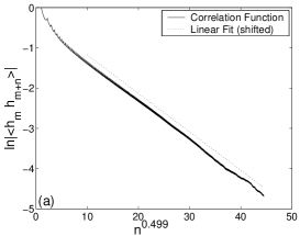
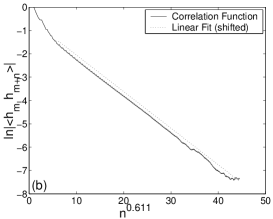
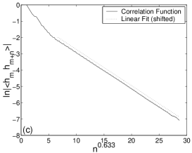
Figure 12: The $r$ dependence of the stretched exponential relation for (a) $r=3.83$, (b) $r=3.87$ and (c) $r=3.9$.

In a sense, it is not surprising that the bound on the values of the fluctuating field does not affect the time decay of the correlations. In the context of glassy systems stretched exponential relaxations of correlation functions were searched and found in kinetically constrained models [49] in which the dynamic variables are naturally bounded (they are spins).

It would be very interesting to test whether a similar stretched exponential relaxation occurs in the confined continuous KPZ equation but this check goes beyond the scope of this article.

5.4 The Lyapunov vector

It was conjectured by Pikovsky et al [27] that the evolution of linear perturbations in the chaotic regime of a CML of logistic elements is well described by the KPZ stochastic dynamics. The notion of a Lyapunov vector is one of the ways to extend the notion of Lyapunov exponent to space-time chaos. One solves simultaneously the original nonlinear dynamical system, and the linearized equation for a perturbation. The Lyapunov exponent is then determined from the norm of the Lyapunov vector.

In the case of the CML, it is convenient to write the linearisation of eq. (2) in the following way

$$\tilde{\omega}({x,t})=f^{\prime}\left[{h({x,t})}\right]\omega({x,t})\;,$$ (37)

$$\omega({x,t+1})=\left({1-\nu}\right)\tilde{\omega}({x,t})+\frac{\nu}{2}\left[\tilde{\omega}({x-1,t})+\tilde{\omega}({x+1,t})\right]\;,$$ (38)

where $\omega(x,t)$ is the Lyapunov vector. using the continuum limit (11)-(14) we obtain the following continuum equation for $\tilde{\omega}(x,t)$:

$$\frac{\partial\tilde{\omega}}{\partial t}=\frac{\nu}{2}\frac{\partial^{2}\tilde{\omega}}{\partial x^{2}}+\left\{f^{\prime}\left[h({x,t+1})\right]-1\right\}\;\left[\tilde{\omega}({x,t})+\frac{\nu}{2}\frac{\partial^{2}\tilde{\omega}}{\partial x^{2}}\right]\;.$$ (39)

We are then led to identify a ‘multiplicative noise’

$$\xi_{\times}\left({x,t}\right)\equiv f^{\prime}\left[{h\left({x,t+1}\right)}\right]-1\;.$$ (40)

(The fact that $f^{\prime}\left[{h\left({x,t+1}\right)}\right]$ is strictly speaking evaluated at time $t+1$ is not a real problem since the process does not depend on the evolution of $\omega(x,t)$, as it does not feed into the equation for the $h$’s. Therefore, one can say that intrinsically the noise in our system should be understood in the Itô sense.)

At this point, since the variable $\tilde{\omega}(x,t)$ is not bounded, a simple scaling argument can convince us that the coupling of the second derivative to the noise $\xi_{x}$ is less relevant (in the RG sense) than the coupling to $\tilde{\omega}(x,t)$ itself. Therefore, we neglect the last term inside the square brackets. The equation we are left with is just a diffusion equation in the presence of multiplicative noise. This motivates the application of the Hopf-Cole transformation, $\tilde{H}=\ln\tilde{\omega}$, which yields

$$\frac{{\partial\tilde{H}}}{{\partial t}}=\frac{\nu}{2}\frac{{\partial^{2}\tilde{H}}}{{\partial x^{2}}}+\frac{\nu}{2}\left({\frac{{\partial\tilde{H}}}{{\partial x}}}\right)^{2}+\xi_{\times}\left({x,t}\right).$$ (41)

Now, we have to figure out the dynamics of $H\equiv\ln\omega$, i.e. the Lyapunov vector. This is easily done by taking the $\ln$ of eq. (37)

$$H\left({x,t}\right)=\tilde{H}({x,t})-\ln f^{\prime}\left[{h\left({x,t}\right)}\right]$$ (42)

This means that $H$ will be just $\tilde{H}$ up to an additional ‘additive noise’, $\xi_{+}\left({x,t}\right)$, defined as

$$\xi_{+}({x,t})\equiv-\ln f^{\prime}\left[{h\left({x,t}\right)}\right]\;.$$ (43)

The roughness of the ‘interface’ $H({x,t})$ is given by the equal-time autocorrelation function of $H({x,t})$. Therefore, we need to check the statistical properties of $\xi_{+}({x,t})$, that is to say, its autocorrelation function and its correlations with $\tilde{H}({x,t})$. We checked that since the term is exponentially distributed, with very short-range correlations in space-time and vanishing correlations with $\tilde{H}({x,t})$, the dominant contribution to the autocorrelation function of $\tilde{H}({x,t})$ comes from $H({x,t})$, and is therefore described by the KPZ exponents. This is not surprising, since the noise $\xi_{+}(x,t)$ does not accumulate in $H(x,t)$, but rather it just adds a random number to $\tilde{H}(x,t)$ with a small amplitude.

This establishes the hypothesis of Pikovsky et al [27] but, more importantly, it allows us to make a step forward relating known quantities in the KPZ literature to features of the Lyapunov exponent. The Lyapunov exponent is obtained from the norm of the Lyapunov vector. If one uses the so-called $0$-norm,

$$N_{0}(t)=\exp\left[\frac{1}{L}\int_{0}^{L}h(x,t)dx\right]\;,$$ (44)

it is then assured to be a self-averaging quantity. In addition, the Lyapunov exponent is given by

$$\lambda=\mathop{\lim}\limits_{T\to\infty}\frac{{\ln N_{0}\left(T\right)-\ln N_{0}\left(0\right)}}{T}\;,$$ (45)

and this is no other than the large-deviation function for the Asymmetric Exclusion Process (ASEP). calculated previously by Derrida and Appert [43]. The ASEP is a discrete model in the universality class as KPZ in one dimension. In terms of the ASEP, the Lyapunov exponent is given by

$$\lambda=\rho\left({1-\rho}\right)+\sqrt{\frac{{\rho\left({1-\rho}\right)}}{{2\pi L^{3}}}}G\left({\sqrt{2\pi\rho\left({1-\rho}\right)L}}\right)$$ (46)

where $L$ is the system size, $\rho$ is a the density of particles (a parameter in ASEP), and $G(\beta)$ is a scaling function independent of $L$ and $\rho$ and known is an implicit form (see [43] for more details).

What is left now is to relate the parameters of the ASEP model to those of the the KPZ equation we derived for $H(x,t)$ (41). Using ref. [44] we see that $\rho(1-\rho)=D/32$ where $D$ is the noise amplitude characterizing $\xi_{\times}(x,t)$. In general, $D$ would be a complicated function of $r$ and $\nu$, and is unknown at the moment. Still, the expression for the Lyapunov exponent (46) could be useful to study finite size effects. As an exercise, we try to estimate $D$ using the known PDF of a single (uncoupled) map, in the fully chaotic regime ($r=4$), given by eq. (20). In that limit $\xi_{\times}=3-8x$, and is known to be uncorrelated in time. Therefore, $D=\langle\xi_{\times}^{2}\rangle=9$. Plugging this into eq. (46) yields $\lambda=9/32\simeq 0.28$. In numerical simulations Pikovsky and Politi found $\lambda\simeq 0.38$ [27] which is of the same order of magnitude as our result. The difference is certainly related to the fact that we approximated $\xi_{\times}$ by that of a single map. In addition, we neglected $\xi_{+}$, and this could have influenced as well.

6 Travelling wave solutions

Let us now briefly analyse the coupled map lattice model and its continuum limit from the viewpoint of front propagation and look for travelling wave configurations linking the two stationary solutions:

$$h=0\;,\qquad\mbox{and}\;\qquad h=\frac{r-1}{r}\;.$$ (47)

The non-linear term $\eta$ renders the solution $h=0$ linearly unstable: $d\eta/dh(h=0)=(r-1)>0$ and the solution $h=(r-1)/r$ stable $d\eta/dh(h=(r-1)/r)<0$ if $r>1/2$. Introducing the travelling wave Ansatz (9) in the linearized version of eq. (15) in which we drop the terms proportional to $F^{2}$, $FF^{\prime\prime}$ and $(F^{\prime})^{2}$ we find

$$v\geq v_{min}\qquad\mbox{with}\qquad v_{min}=\sqrt{2\nu r(r-1)}\;,$$ (48)

and $\gamma_{min}=\sqrt{2(r-1)/(\nu r)}$. The combined effect of the diffusion and non-linear term of KPZ type are not obvious but one may expect that if we start with a localized initial condition with, e.g., the form of a bump with $h\neq 0$ in a finite region of the one dimensional space, the non-linear term will drive the border of the bump into the unstable state $h=0$. The front may then advance as a travelling wave.

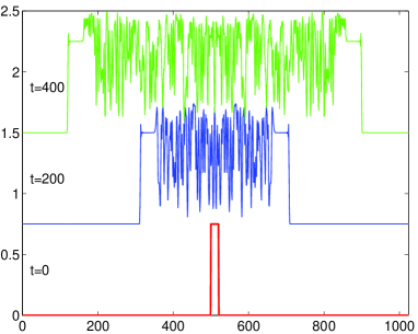
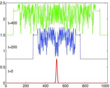
Figure 13: Evolution of the initial configurations for (a) a step-like initial condition and (b) a Gaussian bump.

In Fig. 13 (a) and (b) we show the evolution of the CML starting from localized configurations with a step-like initial condition in panel (a) and a Gaussian form in panel (b). The configuration $x_{n}^{i}$ at three times, $n=0$, $n=200$ and $n=400$ are shown with different lines. They have been translated vertically to render the identification of the curves simpler. For both initial conditions, after a very short transient the configuration acquires rather sharp borders with a ‘random’-like form within the step. More precisely, the value at the plateau close to the borders is well described by the stable solution $x^{i}_{n}\sim(r-1)/r=3/4$ while the values of the random-looking peaks on this plateau have an average $\langle\,x\,\rangle\sim 0.67$ as in Sect. 5.2. For these times the decay to zero at the edges is very sharp, it occurs in less than 10 lattice spacings.

In Fig. 14 we display the evolution of the CML starting now from a more extended initial conditions; more precisely, we took an exponentially decaying form $e^{-x/\xi}$ with $\xi=8$, and we show the configuration $x_{n}^{i}$ at three times $n=0$, $n=20$, and $n=40$. It is clear that the front travels much faster in this case than in the examples studied in Fig. 13. Moreover, the interface is not as sharp.

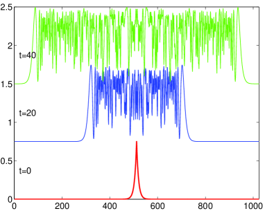
Figure 14: Evolution of the initial configurations for an exponentially decaying initial condition.

We delay for future work [54] a quantitative analysis of the velocity of propagation. One might expect that additional non-linearities, as the KPZ-like term, can only increase (or leave unchanged) the velocity with respect to $v_{min}$. A sufficient condition to have a pulled front is that all non-linear terms should suppress growth for a front that propagates into a linearly unstable state. In our modified FKPP equation it is not obvious a priori whether this holds.

7 Conclusions

We have shown that in the continuum space and time limits the CML of logistic units in $d=1$ becomes an equation of the KPZ type. We argued that some non-linear terms have a triple effect. These terms can be interpreted as a noise source with short-range correlations in time and space, an assumption that we supported with the statistical analysis of numerically generated configurations. But they also provide a source for confinement thus reducing considerably the roughness of the surface: the positive roughness exponent $\alpha$ found in conventional KPZ is reduced to a vanishing value. On the other hand, the same non-linear terms have the form encountered in the FKPP equation for the diffusion of advantageous genes and one can then expect to find travelling wave configurations in the discrete model. We also argued that the field-dependent viscosity appearing in the partial differential equation has no special effect.

As regards to time-dependent observables in the CML, we found that the correlations in time of the local fluctuations have a stretched exponential decay as recently claimed to arise for surfaces generated by the conventional (unbounded) KPZ equation [38]-[40].

We have shown results for the pair of parameters $\nu=0.4$ and $r=4$ where the system is deep in the chaotic regime. A detailed analysis of the phase diagram is beyond the scope of this article. We just mention that the stretched exponential decay persists when keeping the value of $\nu$ fixed and reducing $r$ until reaching the ‘critical’ value $r\approx 3.83$. Interestingly enough, long periods of local blocking are not necessary to find such a slow relaxation since we find it even when the space-time plots look extremely chaotic. Time correlations are hidden in these plots.

A number of authors have signalled the possible relevance of CMLs in describing different aspects of glassy relaxation. Recently, Mousseau et al [45, 46] studied the same model in its intermittent regime ($\nu=0.4,\;r\approx 3.83$) with the aim of relating the 10 orders of magnitude stretched exponential decay of its distribution of trapping times (times in which an element remains locked into one of the coarse-grained values $s_{n}^{i}=\pm 1$) to the one observed in super-cooled liquids. Simdyankin and Mousseau  [46] associated this stretched exponential decay to the one of the correlation function. As we have already stressed, we also obtain a stretched exponential relaxation for larger value of $r$ where trapping intervals for the coarse-grained variables $s_{n}^{i}$ do not exist (see Fig. 1). In a similar spirit to the works of Mousseau, Garrahan and Chandler associated [50] the slow dynamics and glass transition to the structure of trajectories, in the form of the space-time maps, of the spin-like variables in kinetically constrained lattice gases (see [51] for a review of these models). A fully-connected model of logistic maps was studied from the glassy point of view by a number of authors; a range of values of $r$ with a large number of ‘macroscopic states’ and ‘ergodicity breaking’ [47] and the possibility of an analog of replica-symmetry-breaking [48] were reported. With the baggage gained from the current understanding of the dynamics of glassy systems [52] we intend to revisit the generation of an effective temperature [8, 10, 53] and its possible appearance in a fluctuation relation [54, 55] in chaotic systems [56].

Finally, we also briefly analysed the resulting partial differential equation in comparison with the FKPP and we showed that the CML has travelling wave solutions with similar qualitative properties to the ones in FKPP. A more detailed analysis is necessary to understand the main characteristics of the front and, in particular, classify its velocity depending on the initial conditions and other parameters.

Acknowledgements We thank H. Chaté, B. Derrida, J. A. González, J. Kurchan, S. Majumdar, N. Mousseau, I. Procaccia, L. Trujillo and F. Zamponi for very helpful discussions. L.F.C. is a member of the Institut Universitaire de France.

References

- [1] See, for instance, Y. Pesin and A. Yurchenko, Some Physical Models of The Reaction-Diffusion Equation and Coupled Map Lattice, Russian Math. Surveys 59 n. 3 (2004). D. R. Orendovici and Ya. B. Pesin, Proceedings of the IMA Volumes in Mathematics and its Applications, Numerical Methods for Bifurcation Problems and Large-scale Dynamical Systems (Springer-Verlag) 119, 327 (1999).
- [2] S. Ulam and J. von Neumann, Bull. Am. Math. Soc. 53, 1120 (1947).
- [3] See, e.g. P. Collet and J.-P. Eckmann, Iterated maps on the interval as dynamical systems, Birkhaeuser, 1980. R. L. Devaney, An introduction to chaotic dynamical systems, 2nd. Ed., Benjamin/Cummings, 1989. C. Preston, Iterates of maps on an interval, Lecture Notes in Mathematics 999, Springer-Verlag, 1983.
- [4] J. A. González, L. I. Reyes, J. J. Suárez, L. E. Guerrero, G. Gutiérrez, Physica A 316, 259 (2002); Physica D 178, 26 (2003).
- [5] Theory and applications of coupled map lattices, K. Kaneko ed., Wiley, New York. Physica D 103, 97 (1993), Chaos 2 (3) (1992).
- [6] L. A. Bunimovich, Physica D 86, 248 (1995).
- [7] L. A. Bunimovich and Ya G. Sinai, Nonlinearity 1, 491 (1988). J. Bricmont and A. Kupiainen, Nonlinearity 8, 379 (1995).
- [8] P. C. Hohenberg and B. I. Shraiman, Physica D 37, 109 (1989).
- [9] B. I. Shraiman, A. Pumir, W. van Saarlos, P. C. Hohenbergm H. Chaté, and M. Holen, Physica D 57, 241 (1992).
- [10] M. S. Bourzutschky and M. C. Cross, Chaos 2, 173 (1992).
- [11] P. Grassberger and T. Schreiber, Physica D 50, 177 (1991).
- [12] J. Miller and D. Huse, Phys. Rev. E 48, 2528 (1993).
- [13] P. Marc, H. Chaté and P. Manneville, Phys. Rev. E 55, 2606 (1997).
- [14] V. Yakhot, Phys. Rev. A 24, 642 (1981).
- [15] V. S. L’vov, V. V. Lebedev, M. Paton, and I. Procaccia, Nonlinearity 6, 25 (1993).
- [16] V. S. L’vov and I. Procaccia, Phys. Rev. Lett. 69, 3543 (1992).
- [17] I. Procaccia, V. S. L’vov, M. H. Jensen, K. Sneppen, and R. Zeitak, Phys. Rev. A 46, 3220 (1992).
- [18] J. M. Hyman, B. Nicolaenko, and S. Zaleski, Physica D 23, 265 (1986). S. Zaleski, Physica D 34, 427 (1989).
- [19] K. Sneppen, J. Krug, M. H. Jensen, C. Jayaprakash, and T. Bohr, Phys. Rev. A 46, R7351 (1992).
- [20] T. Bohr, G. Grinstein, C. Jayaprakash, M. H. Jensen, and D. Mukamel, Phys. Rev. A 46, 4791 (1992).
- [21] R. Kapral, R. Livi, G. Oppo, and A. Politi, Phys. Rev. E 49, 2009 (1994).
- [22] Y. Kuramoto, Chemical oscillations, waves and turbulence (Springer, Berlin, 1984).
- [23] G. I. Sivashinsky, Acta Astron. 4, 1177 (1977).
- [24] M. Kardar, G. Parisi, and Y-C Zhang, Phys. Rev. Lett. 56, 889 (1986).
- [25] J. M. Burgers, The non-linear diffusion equation (Rindel, Boston, 1974).
- [26] A-L Barábasi and H. E. Stanley, Fractal concepts in surface growth (Cambridge University Press, Melbourne, 1992).
- [27] A. S. Pikovsky and J. Kurths, Phys. Rev. E 49, 898 (1994). A. S. Pikovsky and A. Politi, Nonlinearity 11, 1049 (1998). L. Baroni, R. Livi, and A. Torcini, Phys. Rev. E 63, 036226 (2001).
- [28] R. A. Fisher, Ann. of Eugenics 7, 355 (1937).
- [29] A. N. Kolmogorov, I. G. Petrovskii, N. S. Piscounov, A study of the diffusion equation with increase in the amount of substance, and its application to a biological problem, Bull. Moscow Univ. Math. Mech 1, 1 (1937) and in selected works of A. N. Kolmogorov, vol. 1, 242 (Kluwer Academic Pub.).
- [30] W. Van Saaloos, Phys. Rep. 386, 29 (2003). D. Panja, Phys. Rep. 393 87 (2004). E. Brunet and B. Derrida, Computer Physics Communications 121, 376 (1999).
- [31] S. Wolfram, A new kind of science, Wolfram Media Inc., 2002.
- [32] S. M. Ulam, A collection of mathemaical problems, Interscience, New York, 1960. P. Stein and S. Ulam, Rosprawy Matematyczne 39, 401 (1964).
- [33] U. Frisch, S. Che, and O. Thual, in Macroscopic modelling of turbulent flows, U. Frisch ed. (Springer, Berlin, 1985).
- [34] H. Chaté and P. Manneville, Europhys. Lett. 17, 291 (1992); Prog. Theor. Phys. 87, 1 (1992). Chaos 2 (3), 307 (1992).
- [35] N. R. Wagner, The logistic lattice in random number generation, Proceedings of the Thirtieth Annual Allerton Conference on Communications, Control, and Computing, University of Illinois at Urbana-Champaign, 1993, 922-931.
- [36] The effect of lower and/or upper walls on the dynamics of interfaces was considered in G. Grinstein, M. A. Muñoz, and Y. Tu, Phys. Rev. Lett. 76, 4376 (1996). Y. Tu, G. Grinstein, and M. A. Muñoz, Phys. Rev. Lett. 78, 274 (1997). M. A. Muñoz and T. Hwa, Europhys. Lett. 41, 147 (1998). O. Al Hammal, D. de los Santos, and M. A. Muñoz, cond-mat/0510038.
- [37] Z. Racz, SPIE Proceedings, Vol. 5112, pp. 248-258 (2003) and references therein. E. Marinari, A. Pagnani, G. Parisi, Z. Racz, Phys. Rev. E 65, 026136 (2002). S.T. Bramwell, J.-Y. Fortin, P.C.W. Holdsworth, S. Peysson, J.-F. Pinton, B. Portelli, M. Sellitto, Phys. Rev. E 63 (2001) 041106.
- [38] F. Colaiori and M. Moore, Phys. Rev. E 63, 057103 (2001); ibid 65, 017105 (2001).
- [39] M. Schwartz and S. F. Edwards, Physica A 312, 363 (2002).
- [40] E. Katzav and M. Schwartz, Phys. Rev. E 69, 052603 (2004).
- [41] E. Katzav and M. Schwartz, unpublished.
- [42] M. Prähofer and H. Spohn, J. Stat. Phys. 115, 255 (2004).
- [43] B. Derrida and C. Appert, J. Stat. Phys. 94, 1 (1999). C. Appert, Phys. Rev. E 61, 2092 (2000).
- [44] B. Derrida and K. Mallick, J. Phys. A: Math. Gen. 30, 1031 (1997).
- [45] E. R. Hunt, P. Gade, and N. Mousseau, Europhys. Lett. 60, 827 (2002). S. I. Simdyankin and N. Mousseau, and E. R. Hunt, Phys. Rev. E 66, 066205 (2002).
- [46] S. I. Simdyankin and N. Mousseau, Phys. Rev. E 68, 041110 (2003).
- [47] A. Crisanti, M. Falcioni, and A. Vulpiani, Phys. Rev. Lett. 76, 612 (1996).
- [48] S. C. Manrubia and A. S. Mikhailov, Europhys. Lett. 53, 451 (2001).
- [49] A. Buhot and J. P. Garrahan, Phys. Rev. E 64, 021505 (2001).
- [50] J. P. Garrahan and D. Chandler, Phys. Rev. Lett. 89, 035704 (2002).
- [51] F. Ritort and P. Sollich, Adv. in Phys. 52 219 (2003).
- [52] L. F. Cugliandolo, in ‘Slow Relaxation and non equilibrium dynamics in condensed matter’, Les Houches Session 77 July 2002, J-L Barrat, J Dalibard, J Kurchan, M V Feigel’man eds.; cond-mat/0210312.
- [53] L. F. Cugliandolo, J. Kurchan, and L. Peliti, Phys. Rev. E 55, 3898 (1997).
- [54] F. Zamponi, F. Bonetto, L. F. Cugliandolo, and J. Kurchan, J. Stat. Mech. P09013 (2005).
- [55] S-I Sasa, nlin.CD/0010026.
- [56] L. F. Cugliandolo, E. Katzav, and F. Zamponi, in preparation.