Survey-propagation decimation through distributed local computations

Abstract

We discuss the implementation of two distributed solvers of the random K-SAT problem, based on some development of the recently introduced Survey Propagation (SP) algorithm. The first solver, called the “SP diffusion algorithm” diffuses as dynamical information the maximum bias over the system, so that variables-nodes can decide to freeze in a self-organized way, each variable taking its decision on the basis of purely local information. The second solver, called the “SP reinforcement algorithm”, makes use of time-dependent external forcings on each variable, which are adapted in time in such a way that the algorithm approaches its estimated closest solution. Both methods allow to find a solution of the random 3-SAT problem in a range of parameters comparable with the best previously described serialized solvers. The simulated time of convergence towards a solution ( if these solvers were implemented on a fully parallel device) grows as $log(N)$.

I Introduction

Recent progress in the statistical physics of disordered systems has provided results of algorithmic interest: the connection between the geometrical structure of the space of solutions in random NP-complete constraint satisfaction problems (CSP) and the onset of exponential regimes in search algorithms TCS ; MPZ has been at least partially clarified. More important, the analytical methods have been converted into a new class of algorithms MZ with very good performance BMZ .

Similarly to statistical physics models, a generic CSP is composed of many discrete variables which interact through constraints, where each constraint involves a small number of variables. When CSPs are extracted at random from non trivial ensembles there appear phase transitions as the constraint density (the ratio of constraints to variables) increases: for small densities the problems are satisfiable with high probability whereas when the density is larger than a critical value the problems become unsatisfiable with high probability. Close to the phase boundary on the satisfiable side, most of the algorithms are known to take (typically) exponential time to find solutions. The physical interpretation for the onset of such exponential regimes in random hard CSP consists in a trapping of local search processes in metastable states. Depending on the models and on the details of the process the long time behaviour may be dominated by different types of metastable states. However a common feature which can be observed numerically is that for simulation times which are sub-exponential in the size of the problem there exists an extensive gap in the number of violated constraints which separates the blocking configurations from the optimal ones. Such behavior can be tested on concrete random instances which therefore constitute a computational benchmark for more general algorithms.

In the last few years there has been a great progress in the study of phase transitions in random CSP which has produced new algorithmic tools: problems which were considered to be algorithmically hard for local search algorithms, like for instance random K-SAT close to a phase boundary, turned out to be efficiently solved by the so called Survey Propagation (SP) algorithm MZ arising from the replica symmetry broken (RSB) cavity approach to CSP. According to the statistical physics analysis, close to the phase transition point the solution space breaks up into many smaller clusters MPZ ; MZ . Solutions in separate clusters are generally far apart. This picture has been confirmed by rigorous results, first on the simple case of the XORSAT problem cocco ; MRZ , and more recently for the satisfiability problem MMZ ; AR . Moreover, the physics analysis indicates that clusters which correspond to partial solutions —which satisfy some but not all of the constraints— are exponentially more numerous than the clusters of complete solutions and act as dynamical traps for local search algorithms. SP turns out to be able to deal efficiently with the proliferation of such clusters of metastable states.

The SP algorithm consists in a message-passing technique which is tightly related to the better known Belief Propagation algorithm (BP) BP —recently applied with striking success in the decoding of error-correcting codes based on sparse graphs encodings M ; RicUrb ; G ; KFL ; LTS ; luby — but which differs from it in some crucial point. The messages sent along the edges of the graph underlying the combinatorial problem describe in a probabilistic way the cluster-to-cluster fluctuations of the optimal assignment for a variable; while BP performs a “white” average over all the solutions, SP tells us which is the probability of picking up a cluster at random and finding a given variable forced to take a specific value within it (“frozen” variable). Once the iterative equations have reached a fixed-point of such probability distributions (called “surveys” because they capture somehow the distribution of the expectation in the different clusters), it becomes possible in general to identify the variables which can be safely fixed and to simplify the problem accordingly MZ ; BMZ . This procedure, which is intrinsically serial, is known as the SP-inspired decimation algorithm (SID).

From the experimental point of view, the SID has been efficiently used to solve many instances in the hard region of different satisfiability problems and of the graph coloring problem, including instances too large for any earlier method MZ . For example, for random 3-SAT, instances close to the threshold, up to sizes of order $10^{7}$ variables were solved and the computational time in this regime was found experimentally to scale roughly as $N(\log N)^{2}$.

In the present manuscript, we show how the SP decimation algorithm can be made fully distributed. This opens the possibility of a parallel implementation which would lead to a further drastic reduction in the computational cost.

The paper is organized as follows: in part II we introduce some notation and the K-SAT problem, in part III we recall the SP algorithm along with the serial decimation procedure, and parts IV and V are devoted to explaining our new parallel solvers, respectively the first one based on information diffusion and the second one based on external forcing on the variables.

II The SAT problem and its factor graph representation

Though the results we shall discuss are expected to hold for many types of CSP, here we consider just one representative case : the K-SAT problem.

A K-SAT formula consists of $N$ boolean variables $x_{i}\in\{0,1\}$ , $i\in\{1,\ldots,N\}$, with $M$ constraints, in which each constraint is a clause, which is the logical OR ($\vee$) of the variables it contains or of their negations.

Solving the K-SAT formula means finding an assignment of the $x_{i}\in\{0,1\}=\{$directed,negated$\}$ which is such that all the $M$ clauses are true. In the literature, such an assignment can indifferently be called solution, satisfying assignment or ground state if one uses the statistical physics jargon.

In the case of randomly generated K-SAT formulas (variables appearing in the clauses chosen uniformly at random without repetitions and negated with probabiliy $1/2$) a sophisticated phase transition phenomenon sets in : when the number of constraints $M=\alpha N$ is small, the solutions of the K-SAT formulas are distributed close one to each other over the whole $N-$dimensional space, and the problem can easily be solved by the use of classical local search algorithms. Conversely, when $\alpha$ is included in a narrow region $\alpha_{d}<\alpha<\alpha_{c}$, the problem is still satisfiable but the now limited solution phase breaks down into an exponential number of clustered components. Solutions become grouped together into clusters which are fart apart one from the other. This range of parameters is known as the hard-SAT phase: classical local search algorithms get trapped by strictly positive energy configurations which are exponentially more numerous than the ground state ones.

A clause $a$ is characterized by the set of variables $i_{1},...,i_{K}$ which it contains, and the list of those which are negated, which can be characterized by a set of $K$ numbers $J^{a}_{i_{r}}\in\{\pm 1\}$ as follows. The clause is written as

$$\left(z_{i_{1}}\vee...\vee z_{i_{r}}\vee...\vee z_{i_{K}}\right)$$ (1)

where $z_{i_{r}}=x_{i_{r}}$ if $J^{a}_{i_{r}}=-1$ and $z_{i_{r}}=\bar{x}_{i_{r}}$ if $J^{a}_{i_{r}}=1$ (note that a positive literal is represented by a negative $J$). The problem is to find whether there exists an assignment of the $x_{i}\in\{0,1\}$ which is such that all the $M$ clauses are true. We define the total cost $C$ of a configuration ${\bf x}=(x_{1},...,x_{N})$ as the number of violated clauses.

In the so called ”factor graph” representation, the SAT problem can be schemed as follows (see Fig. 1). Each of the $N$ variables is associated to a vertex in the graph, called a “variable node” (circles in the graphical representation), and each of the $M$ clauses is associated to another type of vertex in the graph, called a “function node” (squares in the graphical representation). A function node $a$ is connected to a variable node $i$ by an edge whenever the variable $x_{i}$ (or its negation) appears in the clause $a$. In the graphical representation, we use a full line between $a$ and $i$ whenever the variable appearing in the clause is $x_{i}$ (i.e. $J^{a}_{i}=-1$), a dashed line whenever the variable appearing in the clause is $\bar{x}_{i}$ (i.e. $J^{a}_{i}=1$).

Throughout this paper, the variable nodes indices are taken in $i,j,k,...$, while the function nodes indices are taken in $a,b,c,...$. For every variable node $i$, we denote by $V(i)$ the set of function nodes $a$ to which it is connected by an edge, by $n_{i}=|V(i)|$ the degree of the node, by $V_{+}(i)$ the subset of $V(i)$ consisting of function nodes $a$ where the variable appears un-negated –the edge $(a,i)$ is a full line–, and by $V_{-}(i)$ the complementary subset of $V(i)$ consisting of function nodes $a$ where the variable appears negated –the edge $(a,i)$ is a dashed line–. $V(i)\setminus b$ denotes the set V(i) without a node $b$. Similarly, for each function node $a$, we denote by $V(a)=V_{+}(a)\cup V_{-}(a)$ the set of neighboring variable nodes, decomposed according to the type of edge connecting $a$ and $i$, and by $n_{a}$ its degree. Given a function node $a$ and a variable node $j$, connected by an edge, it is also convenient to define the two sets: $V^{s}_{a}(j)$ and $V^{u}_{a}(j)$, where the indices $s$ and $u$ respectively refer to the neighbors which tend to make variable $j$ respectively satisfy or unsatisfy the clause $a$, defined as (see Fig. 1):

if $$J_{j}^{a}=1\;:\;\ V^{u}_{a}(j)=V_{+}(j)\ \ ;\ \ V^{s}_{a}(j)=V_{-}(j)\setminus a$$ (2)

if $$J_{j}^{a}=-1:\;\ V^{u}_{a}(j)=V_{-}(j)\ \ ;\ \ V^{s}_{a}(j)=V_{+}(j)\setminus a$$ (3)

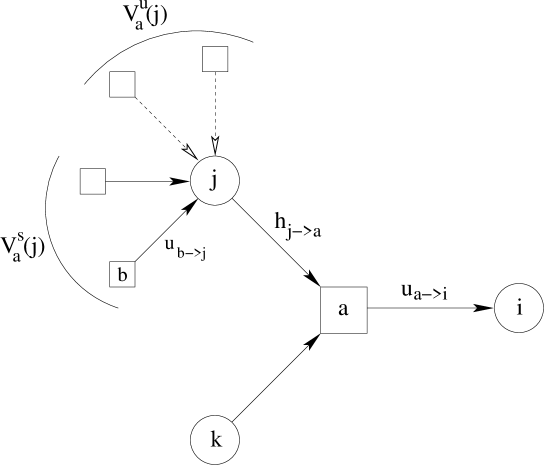
Figure 1: A function node $a$ and its neighborhood. The survey of the cavity-bias $u_{a\to i}$ can be computed from the knowledge of the joint probability distribution for all the cavity-biases in the set $U$, i.e. those coming onto all variable nodes $j$ neighbors of $a$ (except $j=i$).

III Survey Propagation

The survey propagation algorithm (SP) is a message passing algorithm in which the messages passed between function nodes and variable nodes have a probabilistic interpretation. Every message is the probability distribution of some warnings. In this section we provide a short self-contained introduction to SP, starting with the definition of warnings. We refer to refs. MPZ ; MZ ; BMZ for the original derivation of SP from statistical physics tools.

III.1 Warnings

The basic elementary message passed from one function node $a$ to a variable $i$ (connected by an edge) is a Boolean number $u_{a\to i}\in\{0,1\}$ called a ‘warning’.

Given a function node $a$ and one of its variable nodes $i$, the warning $u_{a\to i}$ is determined from the warnings $u_{b\to j}$ arriving on all the variables $j\in V(a)\setminus i$ according to:

$$u_{a\to i}=\prod_{j\in V(a)\setminus i}\theta\left(-J^{a}_{j}\left(\sum_{b\in V(j)\setminus a}J^{b}_{j}u_{b\to j}\right)\right)\ ,$$ (4)

where $\theta(x)=0$ if $x\leq 0$ and $\theta(x)=1$ if $x>0$.

A warning $u_{a\to i}=1$ can be interpreted as a message sent from function node $a$, telling the variable $i$ that it should adopt the correct value in order to satisfy clause $a$. This is decided by $a$ according to the warnings which it received from all the other variables $j$ to which it is connected: if $\left(\sum_{b\in V(j)\setminus a}J^{b}_{j}u_{b\to j}\right)J^{a}_{j}<0$, this means that the tendency for site $j$ (in the absence of $a$) would be to take a value which does not satisfy clause $a$. If all neighbors $j\in V(a)\setminus i$ are in this situation, then $a$ sends a warning to $i$.

The simplest message passing algorithm one can think of is just the propagation of warnings, in which the rule (4) is used as an update rule which is implemented sequentially. The interest in WP largely comes from the fact that it gives the exact solution for tree-problems. In more complicated problems where the factor graph is not a tree, it turns out that WP is unable to converge whenever the density of constraints is so large that the solution space is clustered. This has prompted the development of the more elaborate SP message passing procedure.

III.2 The algorithm

A message of SP, called a survey, passed from one function node $a$ to a variable $i$ (connected by an edge) is a real number $\eta_{a\to i}\in[0,1]$. The interpretation of the survey $\eta_{a\to i}$ is a probability among all clusters of satisfying assignments that a warning is sent from $a$ to $i$.

The SP algorithm uses a random sequential update (see Alg. 1), which calls the local update rule SP-UPDATE (Alg. 2):

Algorithm 1 : SP

Algorithm 2 : subroutine SP-UPDATE$(\eta_{a\to i})$

Whenever the SP algorithm converges to a fixed-point set of messages $\eta_{a\to i}^{*}$, one can use it in a decimation procedure in order to find a satisfiable assignment, if such an assignment exists. This procedure, called the survey inspired decimation (SID) is described in Alg. 3.

Algorithm 3 : SID

There exist several variants of this algorithm. In the code which is available at webserie , for performance reasons we update simultaneously all $\eta$ belonging to the same clause. The clauses to be updated are chosen in a random permutation order at each iteration step. The algorithm can also be randomized by fixing, instead of the most biased variables, one variable randomly chosen in the set of the x percent variables with the largest bias. This strategy allows to use some restart in the case where the algorithm has not found a solution. A fastest decimation can also be obtained by fixing in the step $12$, instead of one variable, a fraction $f$ of the $N_{t}$ variables (the most polarized ones) which have not yet been fixed (going back to $1$ variable when $fN_{t}<1$).

In Ref. BMZ , experimental results are reported which show that SID is able to solve efficiently huge SAT instances very close to the threshold. More specifically, the data discussed in Ref. BMZ show that if SID fixes at each step only one variable, it converges in $\Theta(N^{2}\log N)$ operations (the time taken by walksat Selman to solve the simplified sub-formula seems to grow more slowly). When a fraction of variables is fixed at each time step, we get a further reduction of the cost to $O(N(\log N)^{2})$ (the second $\log$ comes from sorting the biases).

In the following sections we show how the SP procedures can be made fully distributed and hence amenable to a parallel implementation.

IV Distributed SP I: Diffusion algorithm

IV.1 Simulating SP in parallel

The SP algoriths described in the preceeding section is by constructions distributed algorithms, since updates of nodes are performed using message passing procedures from nearest neighbors. However when one uses the surveys in order to find the SAT assignments, in the SID procedure, the decimation process breaks this local information exchange design: it requires a global information, namely the maximally polarization field, used to decide which node has to be frozen at first. It is the purpose of this section to define a procedure able to diffuse such a global information, by using the message passing procedure.

In the present distributed implementation of SP (see Alg. 4), each node is responsible for its own information, any sort of centralized information is prohibited. The information stored at a given function node $a$ is the set of surveys $\{\eta_{a\to i},i\in V(a)\}$. In turn, a given variable node $i$, keeps an information which is the set of cavity-fields $\{\Pi_{i\to a},a\in V(i)\}$. The scheme amounts to implement a message passing procedure such that function nodes send their $\{\eta\}$ values to neigbouring variables nodes, and variable nodes send their fields values in return. Each time a node receives a message from its neighbours, it has to update its own information, accordingly to the survey propagation equations. The broadcasting of information for each individual node is supposed to occur at random. Our simulation proceeds by random updating of each variable or function node. The update time-scale, that is the rate at which nodes in a distributed implementation are able to collect new information and perform their own update will be denoted by $\tau$. Typically, as we shall see the full decimation process is of the order of $10^{4}\tau$, which means that in average each node has to update $10^{4}$ time before the process is completed.

Algorithm 4 : diffusive decimation algorithm

Algorithm 5 : subroutine VARIABLE-NODE-UPDATE

Algorithm 6 : subroutine FUNCTION-NODE-UPDATE

IV.2 Propagation of information

Messages can contain additional information to the one needed to run sp. In the present case, the decimation procedure diffuses the information concerning the highest polarization fields $H_{max}=\text{Max}(|W^{+}-W^{-}|)$ in the system, in order that the variable node, being aware to be the most polarized one, can decide to freeze its assignment to the one given by the orientation of the polarization field.

A static information can freely propagate by simply diffusing in the network, and any component of the network should be informed by a time which has to be proportional to $\log(N)$, $N$ being the size (number of variables nodes) of the system. The difficulty is that the information to be broadcasted may still vary with time before the system has reached equilibrium. The difficulty in propagating a signal saying that the system has converged, might be even more severe. Indeed this amounts to propagate the maximum displacement from the last update of each individual node, which is by essence a transient information.

To take advantage of the basic message-passing procedure, in the case in which the information to be diffused can vary with time, we have to add a mechanism able to suppress obsolete information. The way we propose to do this is to incorporate some damping factor in the broadcasted values.

Let us call $\delta\ll 1$ this damping factor. The procedure goes as follows (see Alg. 5) Each node ($a$ for a function node or $i$ for a variable node) stores its own estimate of the max polarization field $H_{max}$ in a local variable $H_{max}(i)$ or $H_{max}(a)$. Consider first a variable node $i$. When this updates, in addition to the set $\{\eta_{b\to i}\}$ from its neighbour function nodes $b$, it collects also the information $H_{max}(b)$ about the maximum, coming from these nodes, compare it to its own estimation $H_{max}(i)$, and also to its own field value $W_{i}=|W_{i}^{+}-W_{i}^{-}|$. In case the new $H_{max}(i)$ estimation indicates that $i$ is not the most polarized variable node ($H_{max}(i)>W_{i}$), $H_{max}(i)$ is multiplied by a factor $(1-\delta)$. If instead, it appears that $i$ might be the most polarized node ($H_{max}(i)=W_{i}$), then $H_{max}(i)$ is kept as it stands, with no damping correction. For a function node, when it updates, we apply this damping factor anyway. The virtue of this damping effect, is to eliminate any false information. Suppose indeed, that at a given time, a strongly polarized variable node diffuses in the network a very high value of $H_{max}$; if after some time this value is not confirmed (because this node converges to a less polarized state), which means that all local fields $W_{i}$ will be smaller than $H_{max}$, and no unit in the network can pretend to be the most polarized one. Then, mechanically the estimation on the maximum will decay at a rate $\delta$, until when a variable node presents a polarization field higher than the decaying false information.
The counterpart is that the damping takes effect spatially on the network. So typically, since the radius of the network scales like $\log(N)$, the distribution of the estimated maximum given by the set $\{H_{max}(i),H_{max}(a)\}$ taken over the network, will be enlarged by some factor $\delta\log(N)$.
As a result when playing with the parameter $\delta$, two contradictory effects are at work:

• either the information diffuses rapidly with a poor precision (large $\delta$),

• either it takes a long time, before a precise information is diffused (small $\delta)$.

When it comes to the decimation procedure, this can be actually turned into an advantage, since it provides us directly with a parameter able to fix, in an heuristic manner, the rate at which the decimation is performed. Each variable node is equipped with a counting variable $n_{su}(i)$ initially set to zero and counting successive updates with the following two conditions:

• the variation since last updtate of the $\Pi_{i}$’s is less than $\epsilon$ (convergence criteria, typically $\epsilon\simeq 10^{-3}$),

• $i$ may consider itself to be the most polarized variable ($H_{max}(i)=|W_{i}^{+}-W_{i}^{-}|$).

When one of these conditions is not satisfied, $n_{su}(i)$ is set to zero. If $n_{su}(i)$ is greater than a parameter $n_{su}(i)$, the variable is allowed to freeze in the direction given by $W_{i}^{+}-W_{i}^{-}$.

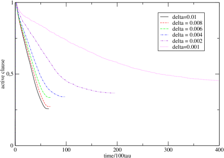
Figure 2: Number of active clauses as a function of time for different values of $\delta$ for a 3-sat problem of size $N=10^{5}$ at $\alpha=4.2$ and $n_{su}=20$.

IV.3 Experimental results

We have simulated the behavior of the algorithm using a standard computer, which allows to monitor how much progress in computing time would be brought by its fully parallel implementation, and to optimize the choices of parameters.

We use the random 3-sat formulas as a benchmark problem. Let N denote the number of variables nodes and $\alpha=M/N$ the ratio of the number of function nodes $M$ over the number of variable nodes. The range of interest is $\alpha\in[4,4.25]$. Simulations are performed with samples of $10^{5}$ function nodes. Figures ( 2, 3, 4, 5) present some average over numerous decimation runs, with various parameters. The runs stop when a paramagnetic state is reached, or when the entropy becomes negative. In order to assess the performance of the algorithm, we measure the simulated time (the time it would take if the computation was really distributed) to reach a paramagnetic state, which can be handled afterwards by walksat in order to find a solution.

The observables which we consider are

• $N_{a}$ the number of active (unfrozen) variables nodes.

• $M_{a}$ the number of active function nodes.

• $\alpha_{2}$ the ratio $M_{a2}/N_{a}$ where $M_{a2}$ is the number of active two-clauses.

• $\alpha_{3}$ the ratio $M_{a3}/N_{a}$ where $M_{a3}$ is the number of active three-clauses. Since we start from a $3-$SAT problem we have of course $M_{a}=M_{a2}+M_{a3}$.

• the entropy of the system, computed from the expression given in BMZ

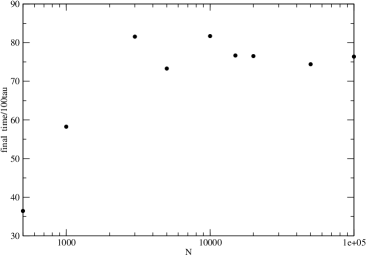
Figure 3: Decimation time up to the paramagnetic state as a function of the size of the system, for a 3-sat problem at $\alpha=4.2$, $\delta=0.005$ and $n_{su}=20$.

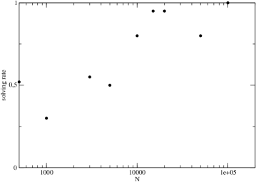
Figure 4: Rate of succesfull decimation process as a function of N for a 3-sat problem at $\alpha=4.2$, $\delta=0.005$ and $n_{su}=20$.

IV.3.1 Orders of magnitude for the tunning parameters

The algorithm depends on two tunable parameters

• the damping factor $\delta$ on the diffusion of information. We find that $\delta\in[0.001,0.01]$ is roughly the range of effectiveness of this parameter for $N=10^{5}$. This actually gives essentially the decimation rate between two convergences of sp. For $\delta\geq 0.01$, too many variables ($\simeq 10^{3}$) are frozen at the same time, and the algorithm ceases to find a paramagnetic state. Instead, when $\delta<0.001$, variables are decimated one by one. The time-dependence of the decimation process with this parameter is illustrated in fig. 2.

• $n_{su}$ the number of successive successful updates needed for a variable, to get frozen. It depends on the precision $\epsilon$ which is required. For $\epsilon=10^{-3}$ it is found that the range of validity of this parameter is between $10$ and $50$. Above $50$, sp converges before the next decimation cascade. Below $20$ the decimation process is essentially continuous. Below $10$ the algorithm ceases to converge to a paramagnetic state.

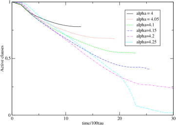
Figure 5: Number of active clauses as a function of time during the decimation process for different values of $\alpha$, for a 3-sat problem of size $N=10^{5}$ at $\delta=0.01$ and $n_{su}=10$.

A reasonable choice for the selection of parameters leading to a fast but still successful decimation procedure is around $\delta=0.01$ and $n_{su}=10$.

IV.3.2 Dependence with the size of the system

Once the typical value for the tunable parameter are determined, it is possible to study the behavior of the algorithm with the sixe of the problem, $N$. Fig. 3, shows that the dependence in $N$ is of the order of $\log N$, which is the best performance one could have with such an algorithm. Another expected result is that rate of successful decimation should increase when $N$ increases, since finite size effect are known to alter efficiency of algorithms for solving 3-sat formulas. This is what is effectively observed in fig. 4

IV.3.3 Dependence with $\alpha$

Depending on $\alpha$ we observe that when we approach the transition point $\alpha_{c}\simeq 4.26$, the final decimation rate increases, (see fig. 5) which is consistent with the hypothesis that the size of the backbone of solutions clusters increases when we approach the critical value of $\alpha$. This can be also visualized when looking at the phase space trajectory of the decimation process (see fig. 6. During the process 2-clauses are generated, which leads to represent the trajectory in the plane $(\alpha_{2},\alpha_{3})$. The trajectory is shorter when we go away from $\alpha_{c}$.

Figure 6: Trajectories in the phase space $(\alpha_{2},\alpha_{3})$ during the decimation process for various values of $\alpha$ for a 3-sat problem of size $N=10^{5}$ at $\delta=0.01$ and $n_{su}=10$. ($5$ samples for each value of $\alpha$, all decimations processes where succesfull up to $\alpha=4.2$, and all failed for $\alpha=4.25$) The slope of the linear part of the trajectories is $\simeq-2.4$.

V Distributed SP II: ’Reinforcement algorithm’

V.1 SP with external forcing field

The SP procedure has recently been generalized to allow the retrieval of a large number of different solutions thanks to the introduction of probability preconditionings BBCZ ; BBCZ2 . The original factor graph is modified applying onto each variable $i$ a constant external forcing survey in direction $\xi_{i}\in\{-1,1\}$ and intensity $\eta_{i}^{ext}=\pi$. An a priori probability $\pi$ of assuming the value $\pm 1$ is being thus assigned to the variable $i$. The components of the forcing modify the usual SP equation (LABEL:eta2) in the following way :

$$\Pi^{\pm}_{j\to a} = \left[1-\left(1-\pi\delta_{\xi_{j},\pm}\right)\prod_{b\in V_{\pm}(j)\setminus a}\left(1-\eta_{b\to j}\right)\right]\cdot$$ (11)

$$\cdot\left(1-\pi\delta_{\xi_{j},\mp}\right)\prod_{b\in V_{\mp}(j)}\left(1-\eta_{b\to j}\right)$$

$$\Pi^{0}_{j\to a} = \left(1-\pi\delta_{\xi_{j},+}\right)\left(1-\pi\delta_{\xi_{j},-}\right)\prod_{b\in V(j)\setminus a}\left(1-\eta_{b\to j}\right)$$

These relations, together with (LABEL:eta1), form the SP equations with external messages (SP-ext). The quantities $\hat{\Pi}_{i}^{+},\hat{\Pi}_{i}^{-},\hat{\Pi}_{i}^{0}$ used to define the local biases on each variable $i$ (see Eq. LABEL:hatpidef) are modified in a similar manner and expressed as a function of the new probabilities $\eta^{*}_{b\to j}$ at the fixed point :

$$\hat{\Pi}^{\pm}_{j\to a} = \left[1-\left(1-\pi\delta_{\xi_{j},\pm}\right)\prod_{b\in V_{\pm}(j)}\left(1-\eta^{*}_{b\to j}\right)\right]\cdot$$ (12)

$$\cdot\left(1-\pi\delta_{\xi_{j},\mp}\right)\prod_{b\in V_{\mp}(j)}\left(1-\eta^{*}_{b\to j}\right)$$

$$\hat{\Pi}^{0}_{j\to a} = \left(1-\pi\delta_{\xi_{j},+}\right)\left(1-\pi\delta_{\xi_{j},-}\right)\prod_{b\in V(j)}\left(1-\eta^{*}_{b\to j}\right)$$

The external messages drive the value of the surveys $\eta^{*}_{a\to i}$ towards the clusters maximally aligned with the external vector field. $\pi=0$ corresponds to the case in which the external messages are absent ; in the case $\pi=1$, the system is fully forced in the direction $\vec{\xi}$. When $\pi$ is correctly chosen, this enables to address more specifically (compared to the SID algorithm, which permits to retrieve only one solution) clusters close to a given region of the $N$-dimensional space. Thus, a right choice of the a priori probability $\pi$, and the use of alternative random directions $\vec{\xi}$ invariably permit to retrieve many solutions in many different clusters.

The criterion used to decimate towards a solution is still the global criterion of the maximum of the magnetization over all variables. So, the decimation based on the SP-ext equations is not yet a distributed solver of the K-SAT formulas.

V.2 Presentation of the method

In order to make the decimation procedure fully distributed, we may adopt time-dependent external messages which are updated according to a reinforcement strategy. More precisely, good properties of convergence are obtained adopting the following scheme :

• in one time step (sweep), all the $\eta$s are parallely updated using the SP equations with external messages(LABEL:eta1, 11), which in this scheme are time-dependent,

• every second time step, one calculates all temporary local fields $\{W_{i}^{(+)},W_{i}^{(-)},W_{i}^{(0)}\}$ using the equations (LABEL:wdef1, LABEL:wdef2, LABEL:wdef3, V.1) —note that these are also functions of the external messages—. The directions $\xi_{i},\>\forall i\in\{1,\ldots,\>N\}$ of the temporary local messages, which are now time-dependent, are parallely updated to equal $sign(W_{i}^{+}-W_{i}^{-})$, i.e. to align itself with the local bias $W_{i}^{+}-W_{i}^{-}$.

As we shall see, with an appropriate choice of the intensity $\pi$ of the forcing, most variables are completely polarized at the end of a single convergence. A solution of the K-SAT formula is finally found by fixing each variable in the direction of its local bias. The reinforcement algorithm (RA) defined above is purely local and hence gives an efficient distributed solver for random K-SAT formulas in the hard-SAT phase.

The algorithm is precisely described in Alg. (7). Its interpretation and a preliminary study of some of its properties are discussed in the subsequent sections.

Algorithm 7 : reinforcement algorithm

Algorithm 8 : subroutine CBS-UPDATE$(\eta_{a\to i})$

Algorithm 9 : subroutine FORC-UPDATE$(\xi_{i})$

To understand how the reinforcement strategy is working, one has to look back at the interpretation of the SP equations with an external forcing survey : imposing an external forcing survey of direction $\xi_{i}\in\{-1,1\}$ on the variable $i$ tries to drive the solution of the cavity biases distributions towards the clusters with a local orientation matching the externally imposed direction $\xi_{i}$.

Then, choosing $\vec{\xi}$ parallel to the vector of the temporary local fields is a strategy which typically guarantees that, if the intensity $\pi$ of the forcing is small enough, the overlap between the forcing vector field $\vec{\xi}$ and the closest solution is continuously increasing, in a stronger way than in the case of the usual SP equations.

When $\pi$ is correctly chosen, some satisfying assignments tend to become stable fixed points of the RA dynamics. The optimal value of $\pi$ is a trade-off between the need for convergence of the SP equations with external forcing survey, the strength of the stabilization induced on the satisfying assignments by the update rule and the amplitude of the perturbation brought by the external forcing. There is a priori no guarantee that there exists a particular value of the intensity $\pi$ for which the algorithm, starting from random initial conditions, gets trapped by a single cluster, and eventually converges to a single solution inside this cluster, without any further decimation. But, our experimental results show that, for $N$ big enough and for almost all values of the parameter $\alpha$ corresponding to the SAT phase, there exists an intensity $\pi$ for which the overlap between the set of local fields and the closest satisfying assignment increases until when it eventually reaches $1$ at the end of a unique convergence.

V.3 Results

V.3.1 Determination of the optimal intensity of the forcing $\pi$

Figure 7: Scaling of the optimized $\pi$ against the complexity $\Sigma$. The optimized $\pi$, which is the intensity of the forcing permitting to find a satisfying assignment in the minimum number of steps, is recalculated for each formula : it depends in average linearly on the complexity : $\pi=11.1\times\Sigma$ ($N=10^{5}$, $K=3$, $4.0<\alpha<4.24$). Each point corresponds to a different formula ; note that the relationship $\pi_{opt}=f(\Sigma)$ becomes slightly sublinear for $\Sigma<0.003$. The subplot shows the evolution of the energy of the dump solution (in which each variable is fixed parallel to the temporary local field) that would be obtained if the convergence was stopped at time $t$ ($\alpha=4.24$).

The efficiency of the method is tested on random 3-SAT formulas. One first determines the optimal intensity $\pi_{opt}$, which is the intensity of the forcing which permits to find a satisfying assignment in the minimum number of steps. When the density of ground states clusters increases (for lower values of $\alpha$), $\pi_{opt}$ should be set at a higher value to be able to bias the convergence towards a unique cluster ; however, a too high value of $\pi$ may let the algorithm converge too rapidly in different parts of the graph towards assignments belonging to different clusters. The algorithm would then loop without convergence among these clusters. For these two reasons, $\pi_{opt}$ should be positively correlated with the complexity $\Sigma=\frac{log(N_{Cl})}{N}$.

One observes that the reinforcement process diverges if the parallel update of the forcings is performed at a too high frequency with respect to the frequency of the parallel updates of the $\eta$s ; the local loops in which the algorithm gets trapped are likely due to simultaneous convergence towards different satisfying assignments in different parts of the graph. A good strategy, systematically used for the experiments of the present paper, is to perform the parallel updates of the forcings once every second parallel update of the $\eta$s.

In the hard-SAT phase, one determines $\pi_{opt}$ as a function of the calculated complexity MZ . As predicted, the experiments show that, for $\alpha_{D}<\alpha<4.245$, $\pi_{opt}$ is positively correlated, and in average scales linearly, with $\Sigma$ ($\pi_{opt}=11.1\times\Sigma$, c.f. Fig. 7, each point representing a different formula), and that the probability of converging towards a satisfying assignment using this value tends to $1$ ($N=10^{5}$, $\epsilon=10^{-3}$, $t_{max}=1000$, c.f. Fig. 8).

V.3.2 Range of validity of the method

Figure 8: Percentage of successful runs (convergence leading to a satisfying assignment) as a function of $\alpha$. The subplot shows the same percentage as a function of the calculated complexity $\Sigma$. The cut-off complexity, for which the RA is successful in half of the cases tested, is $\Sigma_{1/2}=0.0013$ ($N=10^{5}$,$\epsilon=10^{-3}$,$t_{max}=1500)$. The range of validity of the reinforcement algorithm thus matches the one of the SID (see text).

In this section we compare RA with the so-called serialized survey propagation-inspired decimation (SID).

The figure 8 plots the percentage of successful runs (i.e. of convergence towards a satisfying assignment after a single run) of both the synchronous and the asynchronous RA as a function of $\alpha$. One calls synchronous RA the algorithm previously described (Alg. 7) in which the update of all $\eta$s, as well as respectively the update of all forcings, are performed simultaneously. Conversely, in the asynchronous RA, the updates are performed sequentially in a random permutation order (note, that, in the latter case, forcings can be updated as frequently as the $\eta$s). For $\alpha=4.24$, both algorithms invariably permit to retrieve a solution. This is in accordance with the result presented in Ref. BMZ , in which the classical SID has been shown to always find a solution by fixing $0.125\%$ of variables after each convergence of the SP equations.

The cut-off value of the complexity $\Sigma$, for which the decimation converges in half of the cases, is $\Sigma_{1/2}=0.0013$ (subplot of Fig. 8). $\Sigma_{1/2}$ was constant for all sizes of the graph $N>2.10^{4}$. When the complexity decreases, the decimation progressively fails. Depending on the value of $\pi$, either it converges towards a set of local fields, which corresponds to a weighted average of the contributions of numerous clusters of solutions ; or, it loops among low energy configurations (usually, for $N=10^{5}$, $\alpha=4.25$, one finally finds assignments of energy $E=0-50$).

Moreover, asymptotically, the numerical critical $\alpha$ above which the SID, without backtracking, should not permit to find a satisfying assignment has been estimated to be $\alpha_{A}=4.252$ P1 , substantially smaller than the theoretical critical value $\alpha_{C}=4.2667$ (for the improvement brought by the backtracking procedure, see P2 ; BMZ ).

One may study the behavior of the RA at $\alpha_{A}$ for $N=10^{6}$. The calculated complexity of the formulas with $N=10^{6}$ and $\alpha=4.252$ equals $\Sigma=0.00133\pm 0.00013$, in agreement with the cut-off complexity determined for formulas of size $N=10^{5}$ (Fig. 8). For $N=10^{6}$ and $\alpha=4.252$, one then sets $\pi_{opt}=10.5\times\Sigma$ (in agreement with the curve of Fig. 7 for $N=10^{5}$). The “reinforcement algorithm” using these parameters nicely permits to converge towards a solution in $10$ out of the $15$ formulas tested.

One concludes that the present algorithm is valid at least in the same range of parameters as the classical SID BMZ .

V.3.3 Which solutions are addressed?

The satisfying assignments found by the present algorithm are highly dependent on the initial conditions, i.e. on the initial random values imposed on the $\eta$s. For different random initial conditions, one converges towards solutions belonging to different clusters.

To know where the found solutions are located, one chooses an instance from a random graph ensemble in which the number of clauses where any given variable appears negated or directed are kept strictly equal (bar-balanced formulas). For such an instance ($N=30000$, $\alpha=3.33$), the clusters of solutions are expected (and have been observed) to be uniformly distributed over the whole N-dimensional space BBCZ2 . The RA is launched in such an instance $800$ times starting from different random conditions. The histogram of the Hamming distances $d(S_{1},S_{2})=\frac{1}{2}(1-\frac{1}{N}\sum_{i}x_{i}^{(S_{1})}x_{i}^{(S_{2})})$ between any two of the 800 solutions peaks at $0.4995$ (with a standard deviation of $0.0118$).

There is no guarantee that the present algorithm is able to address all clusters of solutions, but the fact that the distance distribution among the found solutions of a bar-balanced formula peaks at $0.5$ with a standard deviation expected from a random distribution (i.e. $\frac{2}{\sqrt{N}}=0.0115$), suggests that the addressable solutions could be homogeneously distributed over the space of the clusters of solutions.

V.3.4 Logarithmic dependence of time on the size of the graph

Figure 9: The number of parallel sweeps needed to find a solution depends logarithmically on $N$ ($\alpha=4.22$, $\pi=0.04$). The examples in which the convergence fails (due to finite size effects, and which have not been observed for $N>30000$) are not represented.

One now analyses the evolution of the convergence time as a function of the size of the graph. For this, one determines, for a fixed value of $\alpha=4.22$, the simulated time that the convergence would take if implemented on a distributed device, as a function of the size $N$ of the graph (Fig. 9). For $N$ ranging from $9000$ to $9.10^{5}$, the time of convergence is well approximated by a logarithmic fit [$t=-315+67*log(N)$]. The unit of time is one parallel update of all $\eta$s. Each point corresponds to a different random formula. Note that, above $N>3.10^{4}$, all trials were successful, and the RA invariably leads to a satisfying assignment. For smaller graphs, due to finite-size effects, the algorithm either fails to converge or converges to an assignment with a few contradictions (generally 1 to 4) in few cases: at most $5\%$ of the experiments for $N=9000$ and none for $N>30000$.

As local messages need a logarithmic time to reach all parts of the graph, and as, in the hard-SAT phase, the assignment of a value to a given variable $i$ does not depend on purely local constraints but on the state of the whole graph, one expects that, by the use of purely local messages on a distributed device, the problem can not be solved faster than in a logarithmic time.

V.3.5 Performance of the reinforcement algorithm on a serialized implementation

Numerical experiments show that RA scales as $N\times\log(N)$ when implemented on a serialized computer. In the scheme of the classical SID, a slightly slower scaling, in $N\times(\log(N))^{2}$, can be achieved by fixing after each convergence a given percentage of the total amount of variable BMZ .

Moreover, Ref. BMZ reports that, for $\alpha=4.24$ and $N=10^{5}$, by fixing at least $f=0.125\%$ of the $N$ variables at the end of each convergence, the SID reaches a paramagnetic state after an average of $7460$ sweeps, i.e. $7460$ updates of all remaining $\eta$s. Conversely, the synchronous RA only needs $600$ parallel updates of the $\eta$s plus $300$ parallel updates of the forcings to converge towards a solution. Its asynchronous version requires $450-500$ complete updates of the $\eta$s and of the forcings to arrive at a solution. This means that, in a serialized computer, close to the critical point, the present algorithm performs faster than the classical SID by a factor of $5$. This can be checked by running the two algorithms on a 2.4 GHz PC : the formula ($N=10^{5}$ and $\alpha=4.24$) is solved in average in $30$ minutes using the SID with $f=0.125\%$ and in $7$ minutes using the “reinforcement algorithm” (either asynchronous or synchronous).

We finally characterize the slowing down of the RA when approaching the critical value $\alpha_{C}=4.2667$ (Fig. 10). Far away from the critical point, the time of convergence is highly reliable. Close to the critical point, the algorithm gets slower and the time of convergence becomes more variable. Setting the intensity of the forcing at its optimal value, one finds that, for $\alpha<\alpha_{A}$, the time of convergence is inversely proportional to the complexity $\Sigma$ : $t=\frac{t_{0}^{\Sigma}}{\Sigma}$ ($t_{0}^{\Sigma}=1.474$, Fig. 10, left panel) ; moreover, as expected from the pseudo-linear relationship between $\Sigma$ and $\alpha$, the time of convergence also scales with $\frac{1}{\alpha-\alpha_{C}}$ : $t=\frac{t_{0}^{\alpha}}{\alpha-\alpha_{C}}$ ($t_{0}^{\alpha}=3.02$, Fig. 10, right panel).

Very close to $\alpha_{C}$ ($\alpha>\alpha_{A}$), the RA is unable to find ground states and only explores quasi-optimal assignments.

Figure 10: Time of convergence as a function of $\Sigma$ (left) or $\alpha$ (right), using for $\pi$ the optimal intensity of the forcing ($N=10^{5}$). Close to the critical point, the time of convergence is shown to be inversely proportional either to $\Sigma$ or to $1-\frac{\alpha}{\alpha_{C}}$. The fit of the datas $t=t_{0}^{\Sigma}\times\Sigma^{-\beta}$ over $\Sigma\in[0,0.008]$ gives $t_{0}^{\Sigma}=1.474$ and $\beta=0.9994$. The fit $t=t_{0}^{\alpha}\times(1-\frac{\alpha}{\alpha_{C}})^{-\gamma}$ over $\alpha\in[4.14,4.25]$ gives $t_{0}^{\alpha}=3.02$ and $\gamma=1.057$.

VI Conclusion

This study aimed at making fully distributed the Survey Propagation decimation algorithm.

The first distributed solver, the “SP diffusion algorithm” diffuses as dynamical information the maximum bias over the system, so that variable-nodes can decide to freeze in a self-organized way. Its properties (solving rate, final number of active clauses when it reaches the paramagnetic state) are comparable with the previously described serialized “SP Inspired Decimation”. The new feature is that the simulated time of convergence towards a solution, if this was implemented on a fully distributed device, goes as $\log(N)$, i.e. scales optimally with the size of the graph.

The second solver, the “SP reinforcement algorithm”, makes use of time-dependent local external forcings, which let the variables get completely polarized in the direction of a solution at the end of a single convergence. The estimated time of convergence of this solver, when implemented on a distributed device, also goes as $\log(N)$.

The present algorithm is the fastest existing solver of the K-SAT formulas, when implemented either on a distributed device chavas or on a serialized computer.

Moreover, the strategies proposed in the present manuscript are not specific to the K-SAT problem, but are likely to apply to many types of NP-complete constraint satisfaction problems (CSP) with direct applications (e.g. data compression algorithm CMZ ).

The different codes are available at (webcyril , webserie ).

Acknowledgements: This work was supported by EVERGROW, integrated project No. 1935 in the complex systems initiative of the Future and Emerging Technologies directorate of the IST Priority, EU Sixth Framework. We thank Demian Battaglia and Alfredo Braunstein for very helpful discussions.

References

- (1) S. Ciliberti, M. Mézard, R. Zecchina, Lossy data compression with random gates, 2005, cond-mat/0504509
- (2) S. Cocco, O. Dubois, J. Mandler, R. Monasson, Rigorous decimation-based construction of ground pure states for spin glass models on random lattices, 2003 Phys. Rev. Lett. 90, 047205
- (3) O. Dubois , R. Monasson, B. Selman and R. Zecchina (Eds.), Phase Transitions in Combinatorial Problems, 2001 Theor. Comp. Sci. 265, 1
- (4) M. Mézard, T. Mora, R. Zecchina, Clustering of solutions in the random satisfiability problem, 2005, cond-mat/0504070
- (5) M. Mézard, F. Ricci-Tersenghi, R. Zecchina, Two solutions to diluted p-spin models and XORSAT problems, 2003 J. Stat. Phys. 111, 505
- (6) D. Achlioptas and F. Ricci-Tersenghi, in preparation
- (7) T. Richardson and R. Urbanke, The capacity of low-density parity-check codes under message-passing decoding, 2001 IEEE Trans Inf. Theory 47 599
- (8) M.G. Luby, M. Mitzenmacher, M.A. Shokrollahi and D.A. Spielman, 2001, 2001 IEEE Trans Inf. Theory 47 585
- (9) D. Battaglia, A. Braunstein, J.Chavas and R.Zecchina, Source Coding by Efficient Selection of Ground States, 2004 submitted to Phys. Rev. E, cond-mat/0412652.
- (10) D.Battaglia, A.Braunstein, J.Chavas and R.Zecchina, Exact Probing of Glassy States by Survey Propagation, 2004 Proceedings of the conference SPDSA-2004, Hayama, Japan.
- (11) A. Braunstein, M. Mézard and R. Zecchina, Survey propagation: an algorithm for satisfiability, 2002 preprint, Random Structures and Algorithms, published on-line in March 2005, cs.CC/0212002
- (12) R.G. Gallager, Low Density Parity Check Codes, 1962 IRE Trans. Inform. Theory 8 21–28
- (13) F.R. Kschischang, B.J. Frey and H.-A. Loeliger, Factor graph and the sum-product algorithm, 2001 IEEE Trans. Inform. Theory 47 498–519
- (14) B. Levine, R.R. Taylor and H. Schmit, Implementation of near Shannon limit error-correcting codes using reconfigurable hardware, 2000 Proc. of the IEEE Symposium on Field-Programmable Custom Computing Machines 217–226
- (15) D.J.C. MacKay, Good error-correcting codes based on very sparse matrices, 1999 IEEE Trans. Inform. Theory 45 399–431
- (16) M. Mézard, G. Parisi and R. Zecchina, Analytic and Algorithmic Solution of Random Satisfiability Problems, 2002 Science 297 812
- (17) M. Mézard and R. Zecchina, The Random K-satisfiability problem : from an analytic solution to an efficient algorithm, 2002 Phys. Rev. E 66, cs.CC/056126
- (18) B. Selman, H. Kautz and B. Cohen, 1994 Proc. AAAI-94 (Seattle, WA), 337–43
- (19) G.Parisi, Some Remarks on the Survey Decimation Algorithm for K-satisfiability, 2003, cs.CC/0301015
- (20) G.Parisi, A backtracking Survey-Propagation Algorithm for K-Satisfiability, 2003, cond-mat/0308510
- (21) J.S. Yedidia, W.T. Freeman and Y. Weiss, Generalized Belief Propagation, 2001 Advances in Neural Information Processing Systems 13 , 689–695, MIT Press
- (22) J. Chavas, D. Battaglia, A. Cicuttin and R. Zecchina, Construction and VHDL implementation of a fully local network with godd reconstruction properties of the inputs, 2005 IWINAC(2) Lecture Notes in Computer Science 3562/2005, 385
- (23) The diffusion code : http://ipnweb.in2p3.fr/~lptms/membres/furtlehn/
- (24) The asynchronous and the synchronous reinforcement code : http://www.ictp.trieste.it/~zecchina/SP/