Nonequilibrium steady states in sheared binary fluids

Abstract

We simulate by lattice Boltzmann the steady shearing of a binary fluid mixture undergoing phase separation with full hydrodynamics in two dimensions. Contrary to some theoretical scenarios, a dynamical steady state is attained with finite domain lengths $L_{x,y}$ in the directions ($x,y)$ of velocity and velocity gradient. Apparent scaling exponents are estimated as $L_{x}\sim\dot{\gamma}^{-2/3}$ and $L_{y}\sim\dot{\gamma}^{-3/4}$. We discuss the relative roles of diffusivity and hydrodynamics in attaining steady state.

Systems that are not in thermal equilibrium play a central role in modern statistical physics, and arise in areas ranging from soap manufacture to subcellular biology SFM . Such systems include two important classes: those that are evolving towards Boltzmann equilibrium (e.g., by phase separation following a temperature quench), and those that are maintained in nonequilibrium by continuous driving (such as a shear flow). Of fundamental interest, and surprising physical subtlety, are systems combining both features — such as a binary fluid undergoing phase separation in the presence of shear. Here it is not known Onuki02 ; Cates99 whether coarsening continues indefinitely, as it does without shear, or whether a steady state is reached, in which the characteristic length scales $L_{x,y,z}$ of the fluid domain structure attain finite $\dot{\gamma}$-dependent values at late times. (We define the mean velocity as $u_{x}=\dot{\gamma}y$ so that $x,y,z$ are velocity, velocity gradient and vorticity directions respectively; $\dot{\gamma}$ is the shear rate.)

Experimentally, saturating length scales are reportedly reached after a period of anisotropic domain growth Hashimoto888994 ; Onuki02 . However, the extreme elongation of domains along the flow direction means that, even in experiments, finite size effects could play an essential role in such saturation Bray03 . Theories in which the velocity does not fluctuate, but does advect the diffusive fluctuations of the concentration field, predict instead indefinite coarsening, with length scales $L_{y,z}$ scaling as $\dot{\gamma}$-independent powers of the time $t$ since quench, and (typically) $L_{x}\sim\dot{\gamma}tL_{y}$ Bray03 . In real fluids, however, the velocity fluctuates strongly in nonlinear response to the advected concentration field, and hydrodynamic scaling arguments, balancing either interfacial and viscous or interfacial and inertial forces, predict saturation (e.g., $L\sim\dot{\gamma}^{-1}$ or $L\sim\dot{\gamma}^{-2/3}$) DoiM91 ; Onuki97 ; Cates99 . Given these experimental and theoretical differences of opinion, computer simulations of sheared binary fluids, with full hydrodynamics, are of major interest.

The aforementioned scaling arguments cannot really distinguish one Cartesian direction from another, but even in theories that can do so, a two dimensional (2D) representation, suppressing $z$, is expected to capture the main physics Bray03 . (Without shear, subtle non-scaling effects arise in 2D from the formation of disconnected droplets WagnerYeomans98 , but shear seems to suppress these WagnerYeomans99 .) Performing simulations in 2D is therefore a fair compromise, especially given the extreme computational demands of the full 3D problem Cates99 ; CatesPT . But, apart from WagnerYeomans99 ; Gonnella01 , most numerical studies of binary fluids under steady shear, even in 2D, neglect hydrodynamics altogether CorberiGL98 ; Lamura01b ; Berthier01 . Among fully hydrodynamic simulations (e.g., WagnerYeomans99 ; Gonnella01 ), only Wagner and Yeomans WagnerYeomans99 make a strong case for dynamical steady states. In some cases these authors found complete remixing of the fluids ($L\rightarrow 0$); in the remainder, finite size effects could not be excluded. (To do so requires $L_{x,y}\ll\Lambda_{x,y}$ for a $\Lambda_{x}\times\Lambda_{y}$ simulation box.) The existence of nonequilibrium steady states, with finite $L_{x,y}$ in an infinite system, therefore remains an open question.

In this letter we extend the hydrodynamic lattice Boltzmann (LB) studies of Refs.WagnerYeomans99 ; Gonnella01 to much larger systems, which we then study over several decades of non-dimensionalized shear rate. Unlike previous authors, we are able to give clear evidence of true dynamical steady states, uncontaminated by finite size effects or other artifacts. (Finite size effects typically result in quasi-laminar stripe domains which connect with themselves after one or more circuits of the periodic boundary conditions WagnerYeomans99 ; CatesPT .) We then combine datasets using a quantitative scaling methodology developed for the unsheared problem in Kendon01 ; this allows scaling exponents to be estimated using combined multi-decade fits. By this method we find apparent scaling exponents $L_{x}\sim\dot{\gamma}^{-2/3},L_{y}\sim\dot{\gamma}^{-3/4}$, sustained over six decades of shear rate.

Our basic LB algorithm for binary fluids is essentially as reported in Kendon01 (see also Swift96 ) on a D2Q9 lattice. Additionally we exploit recent algorithmic advances WagPag ; Adhikari05 that overcome the intrinsic fluid velocity limit of LB by using blockwise translating lattice slabs connected by multiple Lees-Edwards boundary conditions WagPag . (Details of our boundary conditions, with validation data, appear in Adhikari05 .) One technical problem that remains within our LB scheme concerns the role of order parameter diffusivity. In the hydrodynamic coarsening regimes of main interest (late times, modest shear rates) this diffusivity should always maintain local equilibrium across fluid interfaces, but never transport significant material across the interior of domains Kendon01 . Under shear when domains are extremely anisotropic, compromise becomes inevitable. We discuss below the implications of this for the interpretation of our apparent scaling exponents.

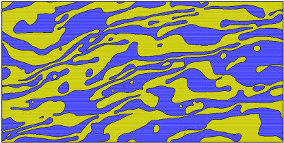
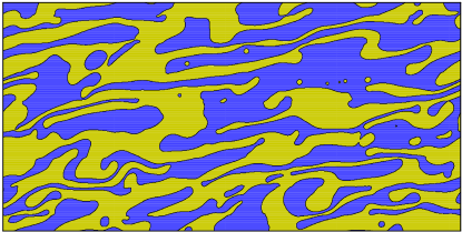
Figure 1: Snapshots of the steady-state order-parameter for R020 with $\dot{\gamma}=0.0005$ at dimensionless times $t\dot{\gamma}=60$ and $255$ (upper and lower).

The governing equations that our LB scheme approximates are the Cahn-Hilliard equation for the compositional order parameter $\varphi$, and the incompressible ($\nabla_{\alpha}u_{\alpha}=0$) Navier-Stokes equation for the velocity $u_{\alpha}$ in an isothermal fluid of unit mass density:

$$\left(\partial_{t}u_{\alpha}+u_{\beta}\nabla_{\beta}u_{\alpha}\right)+\nabla_{\alpha}p-\nu\nabla^{2}u_{\alpha}-\phi\nabla_{\alpha}\mu = 0$$ (1)

$$\partial_{t}\varphi+\nabla_{\alpha}\left(\varphi u_{\alpha}-M\nabla_{\alpha}\mu\right) = 0$$ (2)

Here $p$ is pressure (related in LB to density fluctuations, which remain small, by an ideal gas equation of state Kendon01 ); $\nu$ is the kinematic viscosity; $M$ is the order-parameter mobility, and $\mu=B\varphi\left(\varphi^{2}-1\right)-\kappa\nabla^{2}\varphi$, the chemical potential. $B$ and $\kappa$ are positive constants; the interfacial tension is $\sigma=(8\kappa B/9)^{1/2}$ and the interfacial width is $\xi_{0}=(2\kappa/B)^{1/2}$ Kendon01 . LB control parameters are $B$, $\kappa$, $M$ and $\nu$ alongside the steady shear rate $\dot{\gamma}$.

Blockwise sheared boundary conditions are imposed Adhikari05 such that $\int_{0}^{\Lambda_{y}}\nabla u_{x}\,dy=\Lambda_{y}\dot{\gamma}$. A fluctuating local velocity field can then arise by nonlinearity, as in experiments WagPag . (We neglect thermal fluctuations in our fluid, as appropriate for dynamics near a zero-temperature fixed point Bray94 .) Under shear we define length scales $L_{x,y}$ using a gradient statistic for $\varphi$ that measures the mean distance between interfaces lying across to the chosen direction WagnerYeomans99 . We also define $L_{\|,\bot}$, with $L_{\|}>L_{\bot}$ by reference to appropriate principal axes. (Ref. Berthier01 finds universality, in a related but nonhydrodynamic system, when lengths are scaled with $L_{\|,\bot}$ but not with $L_{x,y}$.)

The physics of binary fluid demixing, with no shear and low enough diffusivity $M$, can be nondimensionalized via a single length scale $L_{0}=\nu^{2}/\sigma$ and time scale $T_{0}=\nu^{3}/\sigma^{2}$. These are, up to dimensionless prefactors Kendon01 , the domain size and time after quench at which an interfacial/viscous balance in the coarsening dynamics (viscous hydrodynamic regime, VH) crosses over to an interfacial/inertial balance (inertial hydrodynamic, IH). By scaling the domain length $L$ and times $t$ by $L_{0}$ and $T_{0}$, multiple datasets were shown to merge, giving a universal crossover between VH and IH regimes Kendon01 ; Pagonabarraga02 .

Accordingly, in our search for nonequilibrium steady states, we nondimensionalize the shear rate as $\dot{\gamma}T_{0}$ and domain sizes as $L_{x,y,\|,\bot}/L_{0}$. One can then expect plots of length against strain rate (or its inverse, as used below) to show data collapse whenever diffusivity is small. One possibility Cates99 is that all such plots might exhibit the same crossover from VH to IH behaviour as would be found by substituting $t=\dot{\gamma}^{-1}$ in the universal scaling plot of $L/L_{0}$ against $t/T_{0}$. This would give $L_{x,y,\|,\bot}\sim L$ with $L/L_{0}\sim(\dot{\gamma}T_{0})^{-1}$ at large shear rates and $L/L_{0}\sim(\dot{\gamma}T_{0})^{-2/3}$ at small ones. Alternatively, some single power law could persist at all $\dot{\gamma}T_{0}$ DoiM91 ; Cates99 ; and/or there could be different exponents in the different directions; or there might be no steady state at all Bray03 .

All simulations reported here were done for fully symmetric quenches on a $\Lambda_{x}\times\Lambda_{y}=1024\times 512$ lattice, with up to $t=6\times 10^{5}$ updates. Parameters $\xi_{0},\sigma,M,\nu$ (Table 1) and $\dot{\gamma}$ were chosen, following Kendon01 , so that: interfaces are wide enough to be resolved (restrictions on $\xi_{0}$); fluid flow is slow enough for advected interfaces to be in local equilibrium (restrictions on $\sigma$ and $\dot{\gamma}$); the diffusivity is low enough not to contaminate steady-state length scales, e.g., detectable as a strong residual $M$ dependence (restriction on $M$). Also, these steady-state lengths must be sufficiently small to avoid finite size effects (quantified below) and the code must run stably for long enough to achieve steady state, typically $t\geq 10^{5}$ updates.

Acceptable shear rates were found to be $1.25\times 10^{-4}\leq\dot{\gamma}\leq 2\times 10^{-3}$ (in lattice units). Higher values gave inaccuracies as listed above; lower values gave unacceptably long run times. As in the unsheared case Kendon01 judicious combinations of $\xi_{0}$, $\sigma$, $M$ and $\nu$ allow systems spanning several decades in $L/L_{0}$ and $\dot{\gamma}T_{0}$ to be accurately studied, by exploiting LB’s ability to vary $L_{0}$ and $T_{0}$ alongside $\dot{\gamma}$.

Name	$\nu$	$M$	$\sigma_{\textrm{theory}}$	$\sigma_{\textrm{meas}}$	$L_{0}$	$T_{0}$
R028	1.41	0.05	0.063	0.055	36.1	927
R022	0.5	0.25	0.047	0.042	5.95	70.9
R029	0.2	0.15	0.047	0.042	0.952	4.54
R020	0.025	2	0.0047	0.0042	0.149	0.886
R030	0.00625	1.25	0.0047	0.0042	0.00930	0.0138
R019	0.0014	4	0.0024	0.0021	0.000933	0.000622
R032	0.0005	5	0.00094	0.00083	0.000301	0.000181

Table 1: Parameter sets used in simulations, along with $L_{0}$ and $T_{0}$. In all cases $\xi_{0}=1.13$. (See Kendon01 for discussion on the difference between the theoretical and measured values of $\sigma$; the measured ones are used to determine $L_{0},T_{0}$).

Fig. 1 shows two snapshots of the order-parameter field for R020 with $\dot{\gamma}=5\times 10^{-4}$ after a steady state had been reached. The snapshots are at dimensionless times $t\gamma=60$ and $t\gamma=255$, for the upper and lower plots respectively. Fig. 2 shows unscaled time-series for $L_{x}$ and $L_{y}$ from a representative set of simulations with $\dot{\gamma}=5\times 10^{-4}$. Both figures show decisive evidence of length-scale saturation in a regime that seems safely clear of any finite size effects. A number of tests were performed in which all run parameters were held constant except the lattice dimensions which were changed in the ranges $\Lambda_{x}=512$ to $2048$ and $\Lambda_{y}=256$ to $1024$. From the results of these tests we conclude that finite-size effects are fully under control when $L_{x,y}\leq\Lambda_{x,y}/4$, a criterion extensively benchmarked in unsheared systems Kendon01 . At the same time, $L_{x,y}\geq 30$ in lattice units, well clear of discretisation artifacts. However, the thin fluid threads visible in Fig. 1 mean that residual diffusion cannot entirely be ruled out; we return to this point below.

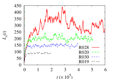
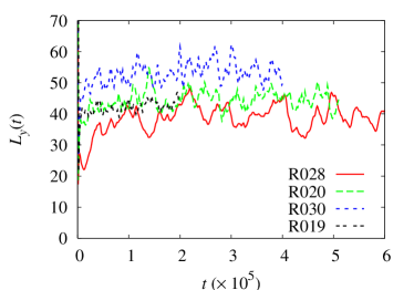
Figure 2: Plots of $L_{x}(t)$ and $L_{y}(t)$ in lattice units, for various runs with $\dot{\gamma}=5\times 10^{-4}$.

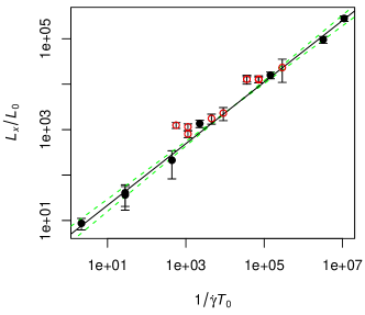
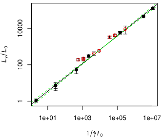
Figure 3: Dimensionless scaling plots of lengths vs shear rate. Error bars as shown give the 95% confidence limits (dashed lines) on the fitted linear regression (solid line). Solid symbols: $\dot{\gamma}=5\times 10^{-4}$. Open symbols have $\dot{\gamma}$ one of, from left to right, $2\times 10^{-3}$, $10^{-2}$, $2.5\times 10^{-4}$ or $1.25\times 10^{-4}$. The fit used only the data for $\dot{\gamma}=5\times 10^{-4}$. Points with two symbols at the same $1/\dot{\gamma}T_{0}$ denote variations in the diffusivity $M$.

Fig. 3 shows dimensionless scaling plots of steady-state length scales $L_{x,y}$ against shear rate, for a series of runs in which $\dot{\gamma}=5\times 10^{-4}$ with variable $L_{0},T_{0}$ (solid symbols). $L_{x,y}$ were obtained as the temporal means of the time-series data $L_{x}(t)$ and $L_{y}(t)$, after discarding data for which $t<10^{5}$. Uncertainties in $L_{x,y}$ (also $L_{\|,\bot}$) were found using 999 bootstrap replicas of the time-series data. These uncertainties, which provide the relative error bars indicated in the scaling plots, were then used to weight the individual data-points in a linear least-squares regression from which estimates were obtained of the intercept and gradient of the straight lines shown on the log-log plots. Fitted exponents for $L_{x}$ and $L_{x}$ are $-0.678\pm 0.042$ and $-0.759\pm 0.029$; and for $L_{\|}$ and $L_{\bot}$, $-0.678\pm 0.039$ and $-0.756\pm 0.030$ (data not shown) footint . The $95$% confidence level admits the appealing ansatz of fractional power laws $L_{x}\sim L_{\|}\sim\dot{\gamma}^{-2/3}$ and $L_{y}\sim L_{\bot}\sim\dot{\gamma}^{-3/4}$.

However, caution is warranted in presenting these apparently clean scaling laws. Firstly, were the dynamic length scales to be found by substituting $t=\dot{\gamma}^{-1}$ in the shear-free coarsening plot as suggested above Cates99 , then a slow crossover from VH ($L\sim\dot{\gamma}^{-1}$) to IH ($L\sim\dot{\gamma}^{-2/3}$) would affect this entire range of $\dot{\gamma}T_{0}$ Kendon01 . Fitting $L_{x,y}$ data to simple power laws might therefore be misleading. Secondly, we also show in Fig. 3 two datasets found by varying $\dot{\gamma}$ with other parameters fixed. For both $L_{x}$ and $L_{y}$, if taken in isolation these sets would suggest smaller slopes than seen for the main plot. Such deviations were found previously in the unsheared case Kendon01 , and argued to be a signature of residual diffusion, with each dataset asymptoting onto the global trend line from above left.

The upward curvature of these two datasets, and the fact that they appear to asymptote onto (rather than cross) the best fit line found for $\dot{\gamma}=5\times 10^{-4}$, offers some reassurance, but no guarantee, that the latter is uncontaminated by residual diffusion at the domain scale. If so, our stationary states stem not from diffusion (although that would itself be interesting) but from the hydrodynamic balance between the stretching, breaking and coalescence of domains. Further evidence for this comes from study of the evolving $\varphi$ field, in which all of these effects are visible but (with our parameters) large-scale diffusion is not. Also, all the simulations reported here quench at $t=0$ from a noisy but uniform state. The system then passes through, and apparently leaves, a diffusive regime prior to the hydrodynamic one that gets cut off by the presence of shear. As a final check, we show directly the effect of varying $M$ in two runs shown in Fig. 3 (where more than one symbol occurs at the same $\dot{\gamma}T_{0}$). The lower data-points were found by reducing $M$ by a factor 2 or more from nearby runs. The resulting shifts are modest, although not entirely negligible — particularly towards the bottom left of the plots. Thus it remains possible that further reduction in $M$ (not practical numerically at present) could reveal a significant kink on these plots, as might be expected near a VH to IH crossover.

In conclusion, although the apparent scaling exponents reported above are interesting and merit both theoretical investigation and experimental tests, the main significance of our work is in the unambiguous demonstration of nonequilibrium steady states in sheared binary fluids. Since theories that neglect velocity fluctuations do not predict such states Bray03 , hydrodynamics appears to play an essential role. (This remains true even if diffusion is not negligible as considered above.) A key question is whether such steady states persist in three dimensions. Although the physics of stretching, breakup and coalescence is captured in 2D, in 3D there can remain tubular connections between domains in the vorticity direction; these could remain relatively unaffected by shear. This might leave open a route to continuous coarsening that is topologically absent in two dimensions. We hope to address the 3D case in future simulations.

Acknowledgements: We thank Ignacio Pagonabarraga and Alexander Wagner for discussions. Work funded by EPSRC GR/S10377 and GR/R67699 (RealityGrid). One of us (JCD) would like to acknowledge the Irish Centre for High-End Computing for access to their computing facilities (SFI grant 04/HEC/I584s1) and support.

References

- (1) M. E. Cates and M. R. Evans (Eds.), Soft and Fragile Matter, Nonequilibrium Dynamics, Metastability and Flow, IOP Publishing, Bristol 2000.
- (2) A. Onuki, Phase Transition Dynamics, Cambridge University Press, Cambridge 2002.
- (3) M. E. Cates, V. M. Kendon, P. Bladon and J-C. Desplat, Faraday Disc. 112, 1 (1999).
- (4) T. Hashimoto, T. Takene and S. Suehiro, J. Chem. Phys. 88, 5875 (1988); C. K. Chan, F. Perrot and D. Beysens, Phys. Rev. A 43, 1826 (1991); A. H. Krall, J. V. Sengers and K. Hamano, Phys. Rev. Lett. 69, 1963 (1992); T. Hashimoto, K. Matsuzaka, E. Moses and A. Onuki, Phys. Rev. Lett. 74, 126 (1995).
- (5) A. J. Bray, Phil. Trans. Roy. Soc. A 361, 781 (2003); A. J. Bray, A. Cavagna and R. D. M. Travasso, Phys. Rev. E 62, 4702 (2000); A. J. Bray and A. Cavagna, J. Phys. A 33, L305 (2000).
- (6) A. Onuki, J. Phys. Cond. Mat. 9, 6119 (1997).
- (7) M. Doi and T. Ohta, J. Chem. Phys. 95, 1241 (1991).
- (8) A. J. Wagner and J. Yeomans, Phys. Rev. Lett. 80, 1429 (1998).
- (9) A. J. Wagner and J. Yeomans, Phys. Rev. E 59, 4366 (1999).
- (10) M. E. Cates, J.-C. Desplat, P. Stansell, A. J. Wagner, K. Stratford, I. Pagonabarraga and R. Adhikari, Phil. Trans. Roy. Soc. A 363, 1917 (2005).
- (11) A. Lamura and G. Gonnella, Physica A 294, 295 (2001).
- (12) F. Corberi, G. Gonnella and A. Lamura Phys. Rev. Lett. 81, 3852 (1998); Phys. Rev. Lett. 83, 4057 (1999); Phys. Rev. E 61, 6621 (2000); Phys. Rev. E 62, 8064 (2000).
- (13) L. Berthier, Phys. Rev. E 63, 051503 (2001).
- (14) A. Lamura, G. Gonnella and F. Corberi, Eur. Phys. J. B 24, 251 (2001).
- (15) V. M. Kendon, M. E. Cates, I. Pagonabarraga, J.-C. Desplat and P. Bladon, J. Fluid Mech. 440, 147 (2001); V. M. Kendon, J.-C. Desplat, P. Bladon and M. E. Cates, Phys. Rev. Lett. 83, 576 (1999).
- (16) M. R. Swift, E. Orlandini, W. R. Osborn and J. M. Yeomans, Phys. Rev. E 54, 830 (1996).
- (17) R. Adhikari, J-C. Desplat and K. Stratford, cond-mat/0503175 (2005).
- (18) A. J. Wagner and I. Pagonabarraga, J. Stat. Phys. 107, 521 (2002).
- (19) A. J. Bray, Adv. Phys. 43, 357 (1994).
- (20) I. Pagonabarraga, A. J. Wagner and M. E. Cates, J. Stat. Phys. 107, 98 (2002).
- (21) The fitted values for the intercepts on the log-log scaling plots are: for , for , for , and for , where the estimated errors represent 95% confidence intervals.