Field Theory Approaches to Nonequilibrium Dynamics

Abstract

It is explained how field-theoretic methods and the dynamic renormalisation group (RG) can be applied to study the universal scaling properties of systems that either undergo a continuous phase transition or display generic scale invariance, both near and far from thermal equilibrium. Part 1 introduces the response functional field theory representation of (nonlinear) Langevin equations. The RG is employed to compute the scaling exponents for several universality classes governing the critical dynamics near second-order phase transitions in equilibrium. The effects of reversible mode-coupling terms, quenching from random initial conditions to the critical point, and violating the detailed balance constraints are briefly discussed. It is shown how the same formalism can be applied to nonequilibrium systems such as driven diffusive lattice gases. Part 2 describes how the master equation for stochastic particle reaction processes can be mapped onto a field theory action. The RG is then used to analyse simple diffusion-limited annihilation reactions as well as generic continuous transitions from active to inactive, absorbing states, which are characterised by the power laws of (critical) directed percolation. Certain other important universality classes are mentioned, and some open issues are listed.

1 Critical Dynamics

Field-theoretic tools and the renormalisation group (RG) method have had a tremendous impact in our understanding of the universal power laws that emerge near equilibrium critical points (see, e.g., Refs. Ramond ; Amit ; ItzDro ; Bellac ; Zinn ; Cardy ), including the associated dynamic critical phenomena HohHalp ; Janssen . Our goal here is to similarly describe the scaling properties of systems driven far from thermal equilibrium, which either undergo a continuous nonequilibrium phase transition or display generic scale invariance. We are then confronted with capturing the (stochastic) dynamics of the long-wavelength modes of the ‘slow’ degrees of freedom, namely the order parameter for the transition, any conserved quantities, and perhaps additional relevant variables. In these lecture notes, I aim to briefly describe how a representation in terms of a field theory action can be obtained for (1) general nonlinear Langevin stochastic differential equations Janssen ; BaJaWa ; and (2) for master equations governing classical particle reaction–diffusion systems JCardy ; MatGlas ; TauHowLee . I will then demonstrate how the dynamic (perturbative) RG can be employed to derive the asymptotic scaling laws in stochastic dynamical systems; to infer the upper critical dimension $d_{c}$ (for dimensions $d\leq d_{c}$, fluctuations strongly affect the universal scaling properties); and to systematically compute the critical exponents as well as to determine further universal properties in various intriguing dynamical model systems both near and far from equilibrium. (For considerably more details, especially on the more technical aspects, the reader is referred to Ref. UCT .)

1.1 Continuous phase transitions and critical slowing down

The vicinity of a critical point is characterised by strong correlations and large fluctuations. The system under investigation is then behaving in a highly cooperative manner, and as a consequence, the standard approximative methods of statistical mechanics, namely perturbation or cluster expansions that assume either weak interactions or short-range correlations, fail. Upon approaching an equilibrium continuous (second-order) phase transition, i.e., for $|\tau|\ll 1$, where $\tau=(T-T_{c})/T_{c}$ measures the deviation from the critical temperature $T_{c}$, the thermal fluctuations of the order parameter $S(x)$ (which characterises the different thermodynamic phases, usually chosen such that the thermal average $\langle S\rangle=0$ vanishes in the high-temperature ‘disordered’ phase) are, in the thermodynamic limit, governed by a diverging length scale

$$\xi(\tau)\sim|\tau|^{-\nu}\ .$$ (1)

Here, we have defined the correlation length via the typically exponential decay of the static cumulant or connected two-point correlation function $C(\vec{x})=\langle S(\vec{x})\,S(0)\rangle-\langle S\rangle^{2}\sim\mathrm{e}^{-|\vec{x}|/\xi}$, and $\nu$ denotes the correlation length critical exponent. As $T\to T_{c}$, $\xi\to\infty$, which entails the absence of any characteristic length scale for the order parameter fluctuations at criticality. Hence we expect the critical correlations to follow a power law $C(x)\sim|x|^{-(d-2+\eta)}$ in $d$ dimensions, which defines the Fisher exponent $\eta$. The following scaling ansatz generalises this power law to $T\not=T_{c}$, but still in the vicinity of the critical point,

$$C(\tau,\vec{x})=|\vec{x}|^{-(d-2+\eta)}\,{\widetilde{C}}_{\pm}(\vec{x}/\xi)\ ,$$ (2)

with two distinct regular scaling functions ${\widetilde{C}}_{+}(\vec{y})$ for $T>T_{c}$ and ${\widetilde{C}}_{-}(\vec{y})$ for $T<T_{c}$, respectively. For its Fourier transform $C(\tau,\vec{q})=\int\!\mathrm{d}^{d}x\,\mathrm{e}^{-{\rm i}\vec{q}\cdot\vec{x}}\,C(\tau,\vec{x})$, one obtains the corresponding scaling form

$$C(\tau,\vec{q})=|\vec{q}|^{-2+\eta}\,{\hat{C}}_{\pm}(\vec{q}\,\xi)\ ,$$ (3)

with new scaling functions ${\hat{C}}_{\pm}(\vec{p})=|\vec{p}|^{2-\eta}\int\!\mathrm{d}^{d}y\,\mathrm{e}^{-{\rm i}\vec{p}\cdot\vec{y}}\,|\vec{y}|^{-(d-2+\eta)}\,{\widetilde{C}}_{\pm}(\vec{y})$.

As we will see in Section 1.5, there are only two independent static critical exponents. Consequently, it must be possible to use the static scaling hypothesis (2) or (3), along with the definition (1), to express the exponents describing the thermodynamic singularities near a second-order phase transition in terms of $\nu$ and $\eta$ through scaling laws. For example, the order parameter in the low-temperature phase ($\tau<0$) is expected to grow as $\langle S\rangle\sim(-\tau)^{\beta}$. Let us consider Eq. (2) in the limit $|\vec{x}|\to\infty$. In order for the $|\vec{x}|$ dependence to cancel, ${\widetilde{C}}_{\pm}(\vec{y})\propto|\vec{y}|^{d-2+\eta}$ for large $|\vec{y}|$, and therefore $C(\tau,|\vec{x}|\to\infty)\sim\xi^{-(d-2+\eta)}\sim|\tau|^{\nu(d-2+\eta)}$. On the other hand, $C(\tau,|\vec{x}|\to\infty)\to-\langle S\rangle^{2}\sim-(-\tau)^{2\beta}$ for $T<T_{c}$; thus we identify the order parameter critical exponent through the hyperscaling relation

$$\beta=\frac{\nu}{2}\,(d-2+\eta)\ .$$ (4)

Let us next consider the isothermal static susceptibility $\chi_{\tau}$, which according to the equilibrium fluctuation–response theorem is given in terms of the spatial integral of the correlation function $C(\tau,\vec{x})$: $\chi_{\tau}(\tau)=(k_{\rm B}T)^{-1}\lim_{\vec{q}\to 0}C(\tau,\vec{q})$. But ${\hat{C}}_{\pm}(\vec{p})\sim|\vec{p}|^{2-\eta}$ as $\vec{p}\to 0$ to ensure nonsingular behaviour, whence $\chi_{\tau}(\tau)\sim\xi^{2-\eta}\sim|\tau|^{-\nu(2-\eta)}$, and upon defining the associated thermodynamic critical exponent $\gamma$ via $\chi_{\tau}(\tau)\sim|\tau|^{-\gamma}$, we obtain the scaling relation

$$\gamma=\nu\,(2-\eta)\ .$$ (5)

The scaling laws (2), (3) as well as scaling relations such as (4) and (5) can be put on solid foundations by means of the RG procedure, based on an effective long-wavelength Hamiltonian ${\cal H}[S]$, a functional of $S(\vec{x})$, that captures the essential physics of the problem, namely the relevant symmetries in order parameter and real space, and the existence of a continuous phase transition. The probability of finding a configuration $S(\vec{x})$ at given temperature $T$ is then given by the canonical distribution

$${\cal P}_{\rm eq}[S]\propto\exp\left(-{\cal H}[S]/k_{\rm B}T\right)\ .$$ (6)

For example, the mathematical description of the critical phenomena for an $O(n)$-symmetric order parameter field $S^{\alpha}(\vec{x})$, with vector index $\alpha=1,\ldots,n$, is based on the Landau–Ginzburg–Wilson functional Ramond ; Amit ; ItzDro ; Bellac ; Zinn ; Cardy

$${\cal H}[S] = \int\!\mathrm{d}^{d}x\sum_{\alpha}\biggl{[}\frac{r}{2}\,[S^{\alpha}(\vec{x})]^{2}+\frac{1}{2}\,[\nabla S^{\alpha}(\vec{x})]^{2}$$ (7)

$$\qquad\qquad+\frac{u}{4!}\,[S^{\alpha}(\vec{x})]^{2}\sum_{\beta}[S^{\beta}(\vec{x})]^{2}-h^{\alpha}(\vec{x})\,S^{\alpha}(\vec{x})\biggr{]}\ ,$$

where $h^{\alpha}(\vec{x})$ is the external field thermodynamically conjugate to $S^{\alpha}(\vec{x})$, $u>0$ denotes the strength of the nonlinearity that drives the phase transformation, and $r$ is the control parameter for the transition, i.e., $r\propto T-T_{c}^{0}$, where $T_{c}^{0}$ is the (mean-field) critical temperature. Spatial variations of the order parameter are energetically suppressed by the term $\sim[\nabla S^{\alpha}(\vec{x})]^{2}$, and the corresponding positive coefficient has been absorbed into the fields $S^{\alpha}$.

We shall, however, not pursue the static theory further here, but instead proceed to a full dynamical description in terms of nonlinear Langevin equations HohHalp ; Janssen . We will then formulate the RG within this dynamic framework, and therein demonstrate the emergence of scaling laws and the computation of critical exponents in a systematic perturbative expansion with respect to the deviation $\epsilon=d-d_{c}$ from the upper critical dimension.

In order to construct the desired effective stochastic dynamics near a critical point, we recall that correlated region of size $\xi$ become quite large in the vicinity of the transition. Since the associated relaxation times for such clusters should grow with their extent, one would expect the characteristic time scale for the relaxation of the order parameter fluctuations to increase as well as $T\to T_{c}$, namely

$$t_{c}(\tau)\sim\xi(\tau)^{z}\sim|\tau|^{-z\nu}\ ,$$ (8)

which introduces the dynamic critical exponent $z$ that encodes the critical slowing down at the phase transition; usually $z\geq 1$. Since the typical relaxation rates therefore scale as $\omega_{c}(\tau)=1/t_{c}(\tau)\sim|\tau|^{z\nu}$, we may utilise the static scaling variable $\vec{p}=\vec{q}\,\xi$ to generalise the crucial observation (8) and formulate a dynamic scaling hypothesis for the wavevector-dependent dispersion relation of the order parameter fluctuations Ferretal ; HalpHoh ,

$$\omega_{c}(\tau,\vec{q})=|\vec{q}|^{z}\,{\hat{\omega}}_{\pm}(\vec{q}\,\xi)\ .$$ (9)

We can then proceed to write down dynamical scaling laws by simply postulating the additional scaling variables $s=t/t_{c}(\tau)$ or $\omega/\omega_{c}(\tau,\vec{q})$. For example, as an immediate consequence we find for the time-dependent mean order parameter

$$\langle S(\tau,t)\rangle=|\tau|^{\beta}\,{\hat{S}}(t/t_{c})\ ,$$ (10)

with ${\hat{S}}(s\to\infty)={\rm const.}$, but ${\hat{S}}(s)\sim s^{-\beta/z\nu}$ as $s\to 0$ in order for the $\tau$ dependence to disappear. At the critical point ($\tau=0$), this yields the power-law decay $\langle S(t)\rangle\sim t^{-\alpha}$, with

$$\alpha=\frac{\beta}{z\,\nu}=\frac{1}{2\,z}\,(d-2+\eta)\ .$$ (11)

Similarly, the scaling law for the dynamic order parameter susceptibility (response function) becomes

$$\chi(\tau,\vec{q},\omega)=|\vec{q}|^{-2+\eta}\,{\hat{\chi}}_{\pm}(\vec{q}\,\xi,\omega\,\xi^{z})\ ,$$ (12)

which constitutes the dynamical generalisation of Eq. (3), for $\chi(\tau,\vec{q},0)=(k_{\rm B}T)^{-1}C(\tau,\vec{q})$. Upon applying the fluctuation–dissipation theorem, valid in thermal equilibrium, we therefrom obtain the dynamic correlation function

$$C(\tau,\vec{q},\omega)=\frac{2k_{\rm B}T}{\omega}\ {\rm Im}\,\chi(\tau,\vec{q},\omega)=|\vec{q}|^{-z-2+\eta}\,{\hat{C}}_{\pm}\left(\vec{q}\,\xi,\omega\,\xi^{z}\right)\ ,$$ (13)

and for its Fourier transform in real space and time,

$$C(\tau,\vec{x},t)=\int\!\frac{\mathrm{d}^{d}q}{(2\pi)^{d}}\!\int\!\frac{\mathrm{d}\omega}{2\pi}\,\mathrm{e}^{{\rm i}(\vec{q}\cdot\vec{x}-\omega t)}\,C(\tau,\vec{q},\omega)=|\vec{x}|^{-(d-2+\eta)}\,{\widetilde{C}}_{\pm}\left(\vec{x}/\xi,t/\xi^{z}\right)\ ,$$ (14)

which reduces to the static limit (2) if we set $t=0$.

The critical slowing down of the order parameter fluctuations near the critical point provides us with a natural separation of time scales. Assuming (for now) that there are no other conserved variables in the system, which would constitute additional slow modes, we may thus resort to a coarse-grained long-wavelength and long-time description, focusing merely on the order parameter kinetics, while subsuming all other ‘fast’ degrees of freedom in random ‘noise’ terms. This leads us to a mesoscopic Langevin equation for the slow variables $S^{\alpha}(\vec{x},t)$ of the form

$$\frac{\partial S^{\alpha}(\vec{x},t)}{\partial t}=F^{\alpha}[S](\vec{x},t)+\zeta^{\alpha}(\vec{x},t)\ .$$ (15)

In the simplest case, the systematic force terms here just represent purely relaxational dynamics towards the equilibrium configuration HaHoMa ,

$$F^{\alpha}[S](\vec{x},t)=-D\,\frac{\delta{\cal H}[S]}{\delta S^{\alpha}(x,t)}\ ,$$ (16)

where $D$ represents the relaxation coefficient, and ${\cal H}[S]$ is again the effective Hamiltonian that governs the phase transition, e.g. given by Eq. (7). For the stochastic forces we may assume the most convenient form, and take them to simply represent Gaussian white noise with zero mean, $\left\langle\zeta^{\alpha}(\vec{x},t)\right\rangle=0$, but with their second moment in thermal equilibrium fixed by Einstein’s relation

$$\left\langle\zeta^{\alpha}(\vec{x},t)\,\zeta^{\beta}(\vec{x}^{\prime},t^{\prime})\right\rangle=2k_{\rm B}T\,D\,\delta(\vec{x}-\vec{x}^{\prime})\,\delta(t-t^{\prime})\,\delta^{\alpha\beta}\ .$$ (17)

As can be verified by means of the associated Fokker–Planck equation for the time-dependent probability distribution ${\cal P}[S,t]$, Eq. (17) guarantees that eventually ${\cal P}[S,t\to\infty]\to{\cal P}_{\rm eq}[S]$, the canonical distribution (6). The stochastic differential equation (15), with (16), the Hamiltonian (7), and the noise correlator (17), define the relaxational model A (according to the classification in Ref. HohHalp ) for a nonconserved $O(n)$-symmetric order parameter.

If, however, the order parameter is conserved, we have to consider the associated continuity equation $\partial_{t}\,S^{\alpha}+\vec{\nabla}\cdot\vec{J}^{\alpha}=0$, where typically the conserved current is given by a gradient of the field $S^{\alpha}$: $\vec{J}^{\alpha}=-D\,\vec{\nabla}S^{\alpha}+\ldots$; as a consequence, the order parameter fluctuations will relax diffusively with diffusion coefficient $D$. The ensuing model B HaHoMa ; HohHalp for the relaxational critical dynamics of a conserved order parameter can be obtained by replacing $D\to-D\,\vec{\nabla}^{2}$ in Eqs. (16) and (17). In fact, we will henceforth treat both models A and B simultaneously by setting $D\to D\,({\rm i}\vec{\nabla})^{a}$, where $a=0$ and $a=2$ respectively represent the nonconserved and conserved cases. Explicitly, we thus obtain

$$\frac{\partial S^{\alpha}(\vec{x},t)}{\partial t} = -D\,({\rm i}\vec{\nabla})^{a}\,\frac{\delta{\cal H}[S]}{\delta S^{\alpha}(\vec{x},t)}+\zeta^{\alpha}(\vec{x},t)$$ (18)

$$= -D\,({\rm i}\vec{\nabla})^{a}\Bigl{[}r-\vec{\nabla}^{2}+\frac{u}{6}\sum_{\beta}[S^{\beta}(\vec{x})]^{2}\Bigr{]}S^{\alpha}(\vec{x},t)$$

$$+D\,({\rm i}\vec{\nabla})^{a}\,h^{\alpha}(\vec{x},t)+\zeta^{\alpha}(\vec{x},t)\ ,$$

with

$$\left\langle\zeta^{\alpha}(\vec{x},t)\,\zeta^{\beta}(\vec{x}^{\prime},t^{\prime})\right\rangle=2k_{\rm B}T\,D\,({\rm i}\vec{\nabla})^{a}\,\delta(\vec{x}-\vec{x}^{\prime})\,\delta(t-t^{\prime})\,\delta^{\alpha\beta}\ .$$ (19)

Notice already that the presence or absence of a conservation law for the order parameter implies different dynamics for systems described by identical static behaviour. Before proceeding with the analysis of the relaxational models, we remark that in general there may exist additional reversible contributions to the systematic forces $F^{\alpha}[S]$, see Sec. 1.6, and / or dynamical mode-couplings to additional conserved, slow fields, which effect further splitting into several distinct dynamic universality classes Cardy ; HohHalp ; UCT .

Let us now evaluate the dynamic response and correlation functions in the Gaussian (mean-field) approximation in the high-temperature phase. To this end, we set $u=0$ and thus discard the nonlinear terms in the Hamiltonian (7) as well as in Eq. (18). The ensuing Langevin equation becomes linear in the fields $S^{\alpha}$, and is therefore readily solved by means of Fourier transforms. Straightforward algebra and regrouping some terms yields

$$\left[-{\rm i}\omega+D\vec{q}^{a}\left(r+\vec{q}^{2}\right)\right]S^{\alpha}(\vec{q},\omega)=D\vec{q}^{a}\,h^{\alpha}(\vec{q},\omega)+\zeta^{\alpha}(\vec{q},\omega)\ .$$ (20)

With $\left\langle\zeta^{\alpha}(\vec{q},\omega)\right\rangle=0$, this gives immediately

$$\chi_{0}^{\alpha\beta}(\vec{q},\omega)=\frac{\partial\langle S^{\alpha}(\vec{q},\omega)\rangle}{\partial h^{\beta}(\vec{q},\omega)}\bigg{|}_{h=0}=D\vec{q}^{a}\,G_{0}(\vec{q},\omega)\,\delta^{\alpha\beta}\ ,$$ (21)

with the response propagator

$$G_{0}(\vec{q},\omega)=\left[-{\rm i}\omega+D\vec{q}^{a}\,(r+\vec{q}^{2})\right]^{-1}\ .$$ (22)

As is readily established by means of the residue theorem, its Fourier backtransform in time obeys causality,

$$G_{0}(\vec{q},t)=\Theta(t)\,\mathrm{e}^{-D\vec{q}^{a}\,(r+\vec{q}^{2})\,t}\ .$$ (23)

Setting $h^{\alpha}=0$, and with the noise correlator (19) in Fourier space

$$\left\langle\zeta^{\alpha}(\vec{q},\omega)\,\zeta^{\beta}(\vec{q}^{\prime},\omega^{\prime})\right\rangle=2k_{\rm B}T\,D\vec{q}^{a}\,(2\pi)^{d+1}\delta(\vec{q}+\vec{q}^{\prime})\,\delta(\omega+\omega^{\prime})\,\delta^{\alpha\beta}\ ,$$ (24)

we obtain the Gaussian dynamic correlation function $\left\langle S^{\alpha}(\vec{q},\omega)\,S^{\beta}(\vec{q}^{\prime},\omega^{\prime})\right\rangle_{0}=C_{0}(\vec{q},\omega)\,(2\pi)^{d+1}\delta(\vec{q}+\vec{q}^{\prime})\,\delta(\omega+\omega^{\prime})$, where

$$C_{0}(\vec{q},\omega)=\frac{2k_{\rm B}TD\vec{q}^{a}}{\omega^{2}+[D\vec{q}^{a}(r+\vec{q}^{2})]^{2}}=2k_{\rm B}T\,D\vec{q}^{a}\,|G_{0}(\vec{q},\omega)|^{2}\ .$$ (25)

The fluctuation–dissipation theorem (13) is of course satisfied; moreover, as function of wavevector and time,

$$C_{0}(\vec{q},t)=\frac{k_{\rm B}T}{r+\vec{q}^{2}}\,\mathrm{e}^{-D\vec{q}^{a}(r+\vec{q}^{2})\,|t|}\ .$$ (26)

In the Gaussian approximation, away from criticality ($r>0$, $\vec{q}\not=0$) the temporal correlations for models A and B decay exponentially, with the relaxation rate $\omega_{c}(r,\vec{q})=D\vec{q}^{2+a}(1+r/\vec{q}^{2})$. Upon comparison with the dynamic scaling hypothesis (9), we infer the mean-field scaling exponents $\nu_{0}=1/2$ and $z_{0}=2+a$. At the critical point, a nonconserved order parameter relaxes diffusively ($z_{0}=2$) in this approximation, whereas the conserved order parameter kinetics becomes even slower, namely subdiffusive with $z_{0}=4$. Finally, invoking Eqs. (12), (13), (14), or simply the static limit $C_{0}(\vec{q},0)=k_{\rm B}T/(r+\vec{q}^{2})$, we find $\eta_{0}=0$ for the Gaussian model.

The full nonlinear Langevin equation (18) cannot be solved exactly. Yet a perturbation expansion with respect to the coupling $u$ may be set up in a slightly cumbersome, but straightforward manner by direct iteration of the equations of motion HaHoMa ; DDBrZJ . More elegantly, one may utilise a path-integral representation of the Langevin stochastic process Jan ; DeDom , which allows the application of all the standard tools from statistical and quantum field theory Ramond ; Amit ; ItzDro ; Bellac ; Zinn ; Cardy , and has the additional advantage of rendering symmetries in the problem more explicit Janssen ; BaJaWa ; UCT .

1.2 Field theory representation of Langevin equations

Our starting point is a set of coupled Langevin equations of the form (15) for mesoscopic, coarse-grained stochastic variables $S^{\alpha}(\vec{x},t)$. For the stochastic forces, we make the simplest possible assumption of Gaussian white noise,

$$\left\langle\zeta^{\alpha}(\vec{x},t)\right\rangle=0\ ,\quad\left\langle\zeta^{\alpha}(\vec{x},t)\,\zeta^{\beta}(\vec{x}^{\prime},t^{\prime})\right\rangle=2L^{\alpha}\,\delta(\vec{x}-\vec{x}^{\prime})\,\delta(t-t^{\prime})\,\delta^{\alpha\beta}\ ,$$ (27)

where $L^{\alpha}$ may represent a differential operator (such as the Laplacian $\vec{\nabla}^{2}$ for conserved fields), and even a functional of $S^{\alpha}$. In the time interval $0\leq t\leq t_{f}$, the moments (27) are encoded in the probability distribution

$${\cal W}[\zeta]\propto\exp\biggl{[}-\frac{1}{4}\int\!\mathrm{d}^{d}x\!\int_{0}^{t_{f}}\!\mathrm{d}t\sum_{\alpha}\zeta^{\alpha}(\vec{x},t)\left[(L^{\alpha})^{-1}\zeta^{\alpha}(\vec{x},t)\right]\biggr{]}\ .$$ (28)

If we now switch variables from the stochastic noise $\zeta^{\alpha}$ to the fields $S^{\alpha}$ by means of the equations of motion (15), we obtain

$${\cal W}[\zeta]\,{\cal D}[\zeta]={\cal P}[S]\,{\cal D}[S]\propto\mathrm{e}^{-{\cal G}[S]}\,{\cal D}[S]\ ,$$ (29)

with the statistical weight determined by the Onsager–Machlup functional BaJaWa

$${\cal G}[S]=\frac{1}{4}\int\!\mathrm{d}^{d}x\!\int\!\mathrm{d}t\sum_{\alpha}\left(\frac{\partial S^{\alpha}}{\partial t}-F^{\alpha}[S]\right)\left[(L^{\alpha})^{-1}\left(\frac{\partial S^{\alpha}}{\partial t}-F^{\alpha}[S]\right)\right]\ .$$ (30)

Note that the Jacobian for the nonlinear variable transformation $\{\zeta^{\alpha}\}\to\{S^{\alpha}\}$ has been omitted here. In fact, the above procedure is properly defined through appropriately discretising time. If a forward (Itô) discretisation is applied, then indeed the associated functional determinant is a mere constant that can be absorbed in the functional measure. The functional (30) already represents a desired field theory action. Since the probability distribution for the stochastic forces should be normalised, $\int\!{\cal D}[\zeta]\,W[\zeta]=1$, the associated ‘partition function’ is unity, and carries no physical information (as opposed to static statistical field theory, where it determines the free energy and hence the entire thermodynamics). The Onsager–Machlup representation is however plagued by technical problems: Eq. (30) contains $(L^{\alpha})^{-1}$, which for conserved variables entails the inverse Laplacian operator, i.e., a Green function in real space or the singular factor $1/\vec{q}^{2}$ in Fourier space; moreover the nonlinearities in $F^{\alpha}[S]$ appear quadratically. Hence it is desirable to linearise the action (30) by means of a Hubbard–Stratonovich transformation BaJaWa .

We shall follow an alternative, more general route that completely avoids the appearance of the inverse operators $(L^{\alpha})^{-1}$ in intermediate steps. Our goal is to average over noise ‘histories’ for observables $A[S]$ that need to be expressible in terms of the stochastic fields $S^{\alpha}$: $\langle A[S]\rangle_{\zeta}\propto\int\!{\cal D}[\zeta]\,A[S(\zeta)]\,W[\zeta]$. For this purpose, we employ the identity

$$1 = \int\!{\cal D}[S]\prod_{\alpha}\prod_{(\vec{x},t)}\,\delta\left(\frac{\partial S^{\alpha}(\vec{x},t)}{\partial t}-F^{\alpha}[S](\vec{x},t)-\zeta^{\alpha}(\vec{x},t)\right)$$ (31)

$$= \int\!{\cal D}[{\rm i}{\widetilde{S}}]\!\int\!{\cal D}[S]\exp\biggl{[}-\int\!\mathrm{d}^{d}x\!\int\!\mathrm{d}t\sum_{\alpha}{\widetilde{S}}^{\alpha}\left(\frac{\partial S^{\alpha}}{\partial t}-F^{\alpha}[S]-\zeta^{\alpha}\right)\biggr{]}\ ,\quad$$

where the first line constitutes a rather involved representation of the unity (in a somewhat symbolic notation; again proper discretisation should be invoked here), and the second line utilises the Fourier representation of the (functional) delta distribution by means of the purely imaginary auxiliary fields ${\widetilde{S}}$ (and factors $2\pi$ have been absorbed in its functional measure).

Inserting (31) and the probability distribution (28) into the desired stochastic noise average, we arrive at

$$\langle A[S]\rangle_{\zeta} \propto \int\!{\cal D}[{\rm i}{\widetilde{S}}]\!\int\!{\cal D}[S]\exp\!\biggl{[}-\!\int\!\mathrm{d}^{d}x\!\int\!\mathrm{d}t\sum_{\alpha}{\widetilde{S}}^{\alpha}\left(\frac{\partial S^{\alpha}}{\partial t}-F^{\alpha}[S]\right)\biggr{]}\,A[S]$$ (32)

$$\times \int\!{\cal D}[\zeta]\exp\biggl{(}-\int\!\mathrm{d}^{d}x\!\int\!\mathrm{d}t\sum_{\alpha}\biggl{[}\,\frac{1}{4}\,\zeta^{\alpha}(L^{\alpha})^{-1}\zeta^{\alpha}-{\widetilde{S}}^{\alpha}\,\zeta^{\alpha}\biggr{]}\biggr{)}\ .$$

We may now evaluate the Gaussian integrals over the noise $\zeta^{\alpha}$, which yields

$$\langle A[S]\rangle_{\zeta}=\int\!{\cal D}[S]\,A[S]\,{\cal P}[S]\ ,\quad{\cal P}[S]\propto\int\!{\cal D}[{\rm i}{\widetilde{S}}]\,\mathrm{e}^{-{\cal A}[{\widetilde{S}},S]}\ ,$$ (33)

with the statistical weight now governed by the Janssen–De Dominicis ‘response’ functional Jan ; DeDom ; BaJaWa

$${\cal A}[{\widetilde{S}},S]=\int\!\mathrm{d}^{d}x\!\int_{0}^{t_{f}}\!\mathrm{d}t\sum_{\alpha}\left[{\widetilde{S}}^{\alpha}\left(\frac{\partial S^{\alpha}}{\partial t}-F^{\alpha}[S]\right)-{\widetilde{S}}^{\alpha}\,L^{\alpha}\,{\widetilde{S}}^{\alpha}\right]\ .$$ (34)

Once again, we have omitted the functional determinant from the variable change $\{\zeta^{\alpha}\}\to\{S^{\alpha}\}$, and normalisation implies $\int\!{\cal D}[{\rm i}{\widetilde{S}}]\int\!{\cal D}[S]\,\mathrm{e}^{-{\cal A}[{\widetilde{S}},S]}=1$. The first term in the action (34) encodes the temporal evolution according to the systematic terms in the Langevin equations (15), whereas the second term specifies the noise correlations (27). Since the auxiliary variables ${\widetilde{S}}^{\alpha}$, often termed Martin–Siggia–Rose response fields MaSiRo , appear only quadratically here, they may be eliminated via completing the squares and Gaussian integrations; thereby one recovers the Onsager–Machlup functional (30).

The Janssen–De Dominicis functional (34) takes the form of a ($d+1$)-dimensional statistical field theory with two independent sets of fields $S^{\alpha}$ and ${\widetilde{S}}^{\alpha}$. We may thus bring the established machinery of statistical and quantum field theory Ramond ; Amit ; ItzDro ; Bellac ; Zinn ; Cardy to bear here; it should however be noted that the response functional formalism for stochastic Langevin dynamics incorporates causality in a nontrivial manner, which leads to important distinctions Janssen .

Let us specify the Janssen–De Dominicis functional for the purely relaxational models A and B HaHoMa ; DDBrZJ , see Eqs. (18) and (19), splitting it into the Gaussian and anharmonic parts ${\cal A}={\cal A}_{0}+{\cal A}_{\rm int}$ BaJaWa , which read

$${\cal A}_{0}[{\widetilde{S}},S] = \int\!\mathrm{d}^{d}x\!\int\!\mathrm{d}t\sum_{\alpha}\biggl{(}{\widetilde{S}}^{\alpha}\left[\frac{\partial}{\partial t}+D\,({\rm i}\vec{\nabla})^{a}\,(r-\vec{\nabla}^{2})\right]S^{\alpha}$$ (35)

$$\qquad\qquad\qquad\quad-D\,{\widetilde{S}}^{\alpha}\,({\rm i}\vec{\nabla})^{a}\,{\widetilde{S}}^{\alpha}-D\,{\widetilde{S}}^{\alpha}\,({\rm i}\vec{\nabla})^{a}\,h^{\alpha}\biggr{)}\ ,$$

$${\cal A}_{\rm int}[{\widetilde{S}},S] = D\,\frac{u}{6}\int\!\mathrm{d}^{d}x\!\int\!\mathrm{d}t\sum_{\alpha,\beta}{\widetilde{S}}^{\alpha}\,({\rm i}\vec{\nabla})^{a}\,S^{\alpha}\,S^{\beta}\,S^{\beta}\ .$$ (36)

Since we are interested in the vicinity of the critical point $T\approx T_{c}$, we have absorbed the constant $k_{\rm B}T_{c}$ into the fields. The prescription (33) tells us how to compute time-dependent correlation functions $\left\langle S^{\alpha}(\vec{x},t)\,S^{\beta}(\vec{x}^{\prime},t^{\prime})\right\rangle$. Using Eq. (35), the dynamic order parameter susceptibility follows from

$$\chi^{\alpha\beta}(\vec{x}-\vec{x}^{\prime},t-t^{\prime})=\frac{\delta\langle S^{\alpha}(\vec{x},t)\rangle}{\delta h^{\beta}(\vec{x}^{\prime},t^{\prime})}\bigg{|}_{h=0}=D\left\langle S^{\alpha}(\vec{x},t)\,({\rm i}\vec{\nabla})^{a}\,{\widetilde{S}}^{\beta}(\vec{x}^{\prime},t^{\prime})\right\rangle\ ;\quad$$ (37)

for the simple relaxational models (only), the response function is just given by a correlator that involves an auxiliary variable, which explains why the ${\widetilde{S}}^{\alpha}$ are referred to as ‘response’ fields. In equilibrium, one may employ the Onsager–Machlup functional (30) to derive the fluctuation–dissipation theorem BaJaWa

$$\chi^{\alpha\beta}(\vec{x}-\vec{x}^{\prime},t-t^{\prime})=\Theta(t-t^{\prime})\,\frac{\partial}{\partial t^{\prime}}\left\langle S^{\alpha}(\vec{x},t)\,S^{\beta}(\vec{x}^{\prime},t^{\prime})\right\rangle\ ,$$ (38)

which is equivalent to Eq. (13) in Fourier space.

In order to access arbitrary correlators, we define the generating functional

$${\cal Z}[{\tilde{j}},j]=\biggl{\langle}\exp\int\!\mathrm{d}^{d}x\!\int\!\mathrm{d}t\sum_{\alpha}\left({\tilde{j}}^{\alpha}\,{\widetilde{S}}^{\alpha}+j^{\alpha}\,S^{\alpha}\right)\biggr{\rangle}\ ,$$ (39)

wherefrom the correlation functions follow via functional derivatives,

$$\biggl{\langle}\prod_{ij}S^{\alpha_{i}}\,{\widetilde{S}}^{\alpha_{j}}\biggr{\rangle}=\prod_{ij}\frac{\delta}{\delta j^{\alpha_{i}}}\,\frac{\delta}{\delta{\tilde{j}}^{\alpha_{j}}}\,{\cal Z}[{\tilde{j}},j]\bigg{|}_{{\tilde{j}}=0=j}\ ,$$ (40)

and the cumulants or connected correlation functions via

$$\biggl{\langle}\prod_{ij}S^{\alpha_{i}}\,{\widetilde{S}}^{\alpha_{j}}\biggr{\rangle}_{c}=\prod_{ij}\frac{\delta}{\delta j^{\alpha_{i}}}\,\frac{\delta}{\delta{\tilde{j}}^{\alpha_{j}}}\,\ln{\cal Z}[{\tilde{j}},j]\bigg{|}_{{\tilde{j}}=0=j}\ .$$ (41)

In the harmonic approximation, setting $u=0$, ${\cal Z}[{\tilde{j}},j]$ can be evaluated explicitly (most directly in Fourier space) by means of Gaussian integration BaJaWa ; UCT ; one thereby recovers (with $k_{\rm B}T=1$) the Gaussian response propagator (22) and two-point correlation function (25). Moreover, as a consequence of causality, $\left\langle{\widetilde{S}}^{\alpha}(\vec{q},\omega)\,{\widetilde{S}}^{\beta}(\vec{q}^{\prime},\omega^{\prime})\right\rangle_{0}=0$.

1.3 Outline of dynamic perturbation theory

Since we cannot evaluate correlation functions with the nonlinear action (36) exactly, we resort to a perturbational treatment, assuming, for the time being, a small coupling strength $u$. The perturbation expansion with respect to $u$ is constructed by rewriting the desired correlation functions in terms of averages with respect to the Gaussian action (35), henceforth indicated with index ’$0$’, and then expanding the exponential of $-{\cal A}_{\rm int}$,

$$\biggl{\langle}\prod_{ij}S^{\alpha_{i}}\,{\widetilde{S}}^{\alpha_{j}}\biggr{\rangle} = \frac{\left\langle\prod_{ij}S^{\alpha_{i}}\,{\widetilde{S}}^{\alpha_{j}}\,\mathrm{e}^{-{\cal A}_{\rm int}[{\widetilde{S}},S]}\right\rangle_{0}}{\left\langle e^{-{\cal A}_{\rm int}[{\widetilde{S}},S]}\right\rangle_{0}}$$ (42)

$$= \biggl{\langle}\prod_{ij}S^{\alpha_{i}}\,{\widetilde{S}}^{\alpha_{j}}\sum_{l=0}^{\infty}\frac{1}{l!}\left(-{\cal A}_{\rm int}[{\widetilde{S}},S]\right)^{l}\biggr{\rangle}_{0}\ .$$

The remaining Gaussian averages, a series of polynomials in the fields $S^{\alpha}$ and ${\widetilde{S}}^{\alpha}$, can be evaluated by means of Wick’s theorem, here an immediate consequence of the Gaussian statistical weight, which states that all such averages can be written as a sum over all possible factorisations into Gaussian two-point functions $\bigl{\langle}S^{\alpha}\,{\widetilde{S}}^{\beta}\bigr{\rangle}_{0}$, i.e., essentially the response propagator $G_{0}$, Eq. (22), and $\bigl{\langle}S^{\alpha}\,S^{\beta}\bigr{\rangle}_{0}$, the Gaussian correlation function $C_{0}$, Eq. (25). Recall that the denominator in Eq. (42) is exactly unity as a consequence of normalisation; alternatively, this result follows from causality in conjunction with our forward descretisation prescription, which implies that we should identify $\Theta(0)=0$. (We remark that had we chosen another temporal discretisation rule, any apparent contributions from the denominator would be precisely cancelled by the in this case nonvanishing functional Jacobian from the variable transformation $\{\zeta^{\alpha}\}\to\{S^{\alpha}\}$.) At any rate, our stochastic field theory contains no ‘vacuum’ contributions.

Figure 1: Elements of dynamic perturbation theory for the $O(n)$-symmetric relaxational models: (a) response propagator; (b) noise vertex; (c) anharmonic vertex.

The many terms in the perturbation expansion (42) are most lucidly organised in a graphical representation, using Feynman diagrams with the basic elements depicted in Fig. 1. We represent the response propagator (22) by a directed line (here conventionally from right to left), which encodes its causal nature; the noise by a two-point ‘source’ vertex, and the anharmonic term in Eq. (36) as a four-point vertex. In the diagrams representing the different terms in the perturbation series, these vertices serve as links for the propagator lines, with the fields $S^{\alpha}$ being encoded as the ‘incoming’, and the ${\widetilde{S}}^{\alpha}$ as the ‘outgoing’ components of the lines. In Fourier space, translational invariance in space and time implies wavevector and frequency conservation at each vertex, see Fig. 2 below. An alternative, equivalent representation uses both the response and correlation propagators as independent elements, the latter depicted as undirected line, thereby disposing of the noise vertex, and retaining the nonlinearity in Fig. 1(c) as sole vertex.

Following standard field theory procedures Ramond ; Amit ; ItzDro ; Bellac ; Zinn , one establishes that the perturbation series for the cumulants (41) is given in terms of connected Feynman graphs only (for a detailed exposition of this and the following results, see Ref. UCT ). An additional helpful reduction in the number of diagrams to be considered arises when one considers the vertex functions, which generalise the self-energy contributions $\Sigma(\vec{q},\omega)$ in the Dyson equation for the response propagator, $G(\vec{q},\omega)^{-1}=D\vec{q}^{a}\,\chi(\vec{q},\omega)^{-1}=G_{0}(\vec{q},\omega)^{-1}-\Sigma(\vec{q},\omega)$. To this end, we define the fields ${\widetilde{\Phi}}^{\alpha}=\delta\ln{\cal Z}/\delta{\tilde{j}}^{\alpha}$ and $\Phi^{\alpha}=\delta\ln{\cal Z}/\delta j^{\alpha}$, and introduce the new generating functional

$$\Gamma[{\widetilde{\Phi}},\Phi]=-\ln{\cal Z}[{\tilde{j}},j]+\int\!\mathrm{d}^{d}x\!\int\!\mathrm{d}t\sum_{\alpha}\left({\tilde{j}}^{\alpha}\,{\widetilde{\Phi}}^{\alpha}+j^{\alpha}\,\Phi^{\alpha}\right)\ ,$$ (43)

wherefrom the vertex functions are obtained via the functional derivatives

$$\Gamma^{({\widetilde{N}},N)}_{\{\alpha_{i}\};\{\alpha_{j}\}}=\prod_{i}^{\widetilde{N}}\frac{\delta}{\delta{\widetilde{\Phi}}^{\alpha_{i}}}\,\prod_{j}^{N}\frac{\delta}{\delta\Phi^{\alpha_{j}}}\,\Gamma[{\widetilde{\Phi}},\Phi]\bigg{|}_{{\tilde{j}}=0=j}\ .$$ (44)

Diagrammatically, these quantities turn out to be represented by the possible sets of one-particle (1PI) irreducible Feynman graphs with $N$ incoming and ${\widetilde{N}}$ outgoing ‘amputated’ legs; i.e., these diagrams do not split into allowed subgraphs by simply cutting any single propagator line. For example, for the two-point functions a direct calculation yields the relations

$$\Gamma^{(1,1)}(\vec{q},\omega) = D\vec{q}^{a}\,\chi(-\vec{q},-\omega)^{-1}=G_{0}(-\vec{q},-\omega)^{-1}-\Sigma(-\vec{q},-\omega)\ ,$$ (45)

$$\Gamma^{(2,0)}(\vec{q},\omega) = -\,\frac{C(\vec{q},\omega)}{|G(\vec{q},\omega)|^{2}}=-\frac{2D\,\vec{q}^{a}}{\omega}\ {\rm Im}\,\Gamma^{(1,1)}(\vec{q},\omega)\ ,$$ (46)

where the second equation for $\Gamma^{(2,0)}$ follows from the fluctuation–dissipation theorem (13). Note that $\Gamma^{(0,2)}(\vec{q},\omega)=0$ vanishes because of causality.

Figure 2: One-loop diagrams for (a) $\Gamma^{(1,1)}$ and (b) $\Gamma^{(1,3)}$ in the time domain.

The perturbation series can then be organised graphically as an expansion in successive orders with respect to the number of closed propagator loops. As an example, Fig. 2 depicts the one-loop contributions for the vertex functions $\Gamma^{(1,1)}$ and $\Gamma^{(1,3)}$ in the time domain with all required labels. One may formulate general Feynman rules for the construction of the diagrams and their translation into mathematical expressions for the $l$th order contribution to the vertex function $\Gamma^{({\widetilde{N}},N)}$:

1. Draw all topologically different, connected one-particle irreducible graphs with ${\widetilde{N}}$ outgoing and $N$ incoming lines connecting $l$ relaxation vertices $\propto u$. Do not allow closed response loops (since in the Itô calculus $\Theta(0)=0$).

2. Attach wavevectors $\vec{q}_{i}$, frequencies $\omega_{i}$ or times $t_{i}$, and component indices $\alpha_{i}$ to all directed lines, obeying ‘momentum (and energy)’ conservation at each vertex.

3. Each directed line corresponds to a response propagator $G_{0}(-\vec{q},-\omega)$ or $G_{0}(\vec{q},t_{i}-t_{j})$ in the frequency and time domain, respectively, the two-point vertex to the noise strength $2D\,\vec{q}^{a}$, and the four-point relaxation vertex to $-D\,\vec{q}^{a}\,u/6$. Closed loops imply integrals over the internal wavevectors and frequencies or times, subject to causality constraints, as well as sums over the internal vector indices. Apply the residue theorem to evaluate frequency integrals.

4. Multiply with $-1$ and the combinatorial factor counting all possible ways of connecting the propagators, $l$ relaxation vertices, and $k$ two-point vertices leading to topologically identical graphs, including a factor $1/l!\,k!$ originating in the expansion of $\exp(-{\cal A}_{\rm int}[{\widetilde{S}},S])$.

Figure 3: One-particle irreducible diagrams for $\Gamma^{(1,1)}(\vec{q},\omega)$ to second order in $u$.

For later use, we provide the explicit results for the two-point vertex functions to two-loop order. After some algebra, the three diagrams in Fig. 3 give

$$\Gamma^{(1,1)}(\vec{q},\omega)={\rm i}\omega+D\vec{q}^{a}\biggl{[}r+\vec{q}^{2}+\frac{n+2}{6}\,u\int_{k}\frac{1}{r+\vec{k}^{2}}$$

$$\qquad\qquad\qquad-\left(\frac{n+2}{6}\,u\right)^{2}\int_{k}\frac{1}{r+\vec{k}^{2}}\int_{k^{\prime}}\frac{1}{(r+{\vec{k}^{\prime}}^{2})^{2}}$$

$$\qquad-\,\frac{n+2}{18}\,u^{2}\int_{k}\frac{1}{r+\vec{k}^{2}}\int_{k^{\prime}}\frac{1}{r+{\vec{k}^{\prime}}^{2}}\,\frac{1}{r+(\vec{q}-\vec{k}-\vec{k}^{\prime})^{2}}$$

$$\qquad\qquad\qquad\times\left(1-\frac{i\omega}{{\rm i}\omega+\Delta(\vec{k})+\Delta(\vec{k}^{\prime})+\Delta(\vec{q}-\vec{k}-\vec{k}^{\prime})}\right)\biggr{]}\ ,$$ (47)

where we have separated out the dynamic part in the last line, and introduced the abbreviations $\Delta(\vec{q})=D\vec{q}^{a}\,(r+\vec{q}^{2})$ and $\int_{k}=\int\!\mathrm{d}^{d}k/(2\pi)^{d}$ UCT .

Figure 4: (a) Two-loop diagram for $\Gamma^{(2,0)}(\vec{q},\omega)$; (b) one-loop graph for $\Gamma^{(1,3)}$.

For the noise vertex, Fig. 4(a) yields UCT

$$\Gamma^{(2,0)}(\vec{q},\omega)=-2D\vec{q}^{a}\biggl{[}1+D\vec{q}^{a}\,\frac{n+2}{18}\,u^{2}\int_{k}\frac{1}{r+\vec{k}^{2}}\int_{k^{\prime}}\frac{1}{r+{\vec{k}^{\prime}}^{2}}$$

$$\qquad\times\frac{1}{r+(\vec{q}-\vec{k}-\vec{k}^{\prime})^{2}}\ {\rm Re}\,\frac{1}{{\rm i}\omega+\Delta(\vec{k})+\Delta(\vec{k}^{\prime})+\Delta(\vec{q}-\vec{k}-\vec{k}^{\prime})}\biggr{]}\ ;\quad$$ (48)

notice that for model B, as a consequence of the conservation law for the order parameter and ensuing wavevector dependence of the nonlinear vertex, see Fig. 1(c), to all orders in the perturbation expansion

$$a=2\,:\ \Gamma^{(1,1)}(\vec{q}=0,\omega)={\rm i}\omega\ ,\quad\frac{\partial}{\partial\vec{q}^{2}}\,\Gamma^{(2,0)}(\vec{q},\omega)\bigg{|}_{\vec{q}=0}=-2D\ .$$ (49)

At last, with the shorthand notation ${\underline{k}}=(\vec{q},\omega)$, the analytical expression corresponding to the graph in Fig. 4(b) for the four-point vertex function at symmetrically chosen external wavevector labels reads

$$\Gamma^{(1,3)}(-3{\underline{k}}/2;\{{\underline{k}}/2\})=D\left(\frac{3}{2}\,\vec{q}\right)^{a}u\biggl{[}1-\frac{n+8}{6}\,u$$

$$\qquad\times\int_{k}\frac{1}{r+\vec{k}^{2}}\,\frac{1}{r+(\vec{q}-\vec{k})^{2}}\left(1-\frac{{\rm i}\omega}{{\rm i}\omega+\Delta(\vec{k})+\Delta(\vec{q}-\vec{k})}\right)\biggr{]}\ .$$ (50)

1.4 Renormalisation

Consider a typical loop integral, say the correction in Eq. (50) to the four-point vertex function $\Gamma^{(1,3)}$ at zero external frequency and momentum, whose ‘bare’ value, without any fluctuation contributions, is $u$. In dimensions $d<4$, one obtains, after introducing $d$-dimensional spherical coordinates and rendering the integrand dimensionless ($x=|\vec{k}|/\sqrt{r}$):

$$u\int\!\frac{\mathrm{d}^{d}k}{(2\pi)^{d}}\,\frac{1}{(r+\vec{k}^{2})^{2}}=\frac{u\,r^{-2+d/2}}{2^{d-1}\pi^{d/2}\Gamma(d/2)}\int_{0}^{\infty}\!\frac{x^{d-1}}{(1+x^{2})^{2}}\,\mathrm{d}x\ ,$$ (51)

where we have inserted the surface area $S_{d}=2\pi^{d/2}/\Gamma(d/2)$ of the $d$-dimensional unit sphere, with Euler’s Gamma function, $\Gamma(1+x)=x\,\Gamma(x)$. Note that the integral on the right-hand side is finite. Thus, we see that the effective expansion parameter in perturbation theory is not just $u$, but the combinaton $u_{\rm eff}=u\,r^{(d-4)/2}$. Far away from $T_{c}$, it is small, and the perturbation expansion well-defined. However, $u_{\rm eff}\to\infty$ as $r\to 0$ for $d<4$: we are facing infrared (IR) divergences, induced by the strong critical fluctuations that render the loop corrections singular. A straightforward application of perturbation theory will therefore not provide meaningful results, and we must expect the fluctuation contributions to modify the critical power laws.

Conversely, for dimensions $d\geq 4$, the integral in (51) develops ultraviolet (UV) divergences as the upper integral boundary is sent to infinity ($k=|\vec{k}|$),

$$\int_{0}^{\Lambda}\!\frac{k^{d-1}}{(r+k^{2})^{2}}\,\mathrm{d}k\sim\left\{\begin{array}[]{cc}\ln(\Lambda^{2}/r)&\quad d=4\\ \Lambda^{d-4}&\quad d>4\end{array}\right\}\to\infty\quad{\rm as}\ \Lambda\to\infty\ .$$ (52)

In lattice models, there is a finite wavevector cutoff, namely the Brillouin zone boundary, $\Lambda\sim(2\pi/a_{0})^{d}$ for a hypercubic lattice with lattice constant $a_{0}$, whence physically these UV problems do not emerge. Yet we shall see that a formal treatment of these unphysical UV divergences will allow us to infer the correct power laws for the physical IR singularities associated with the critical point. The borderline dimension that separates the IR and UV singular regimes is referred to as upper critical dimension $d_{c}$; here $d_{c}=4$. Note that at $d_{c}$, UV and IR singularities are intimately connected and appear in the form of logarithmic divergences, see Eq. (52). The situation is summarised in Table 1, where we have also stated that models with continuous order parameter symmetry, such as the Hamiltonian (7) with $n\geq 2$, do not allow long-range order in dimensions $d\leq d_{\rm lc}=2$ (Mermin–Wagner–Hohenberg theorem Wagner ; MerWag ; Hohenb ). Here, $d_{\rm lc}$ is called the lower critical dimension; for the Ising model represented by Eq. (7) with $n=1$, of course $d_{\rm lc}=1$.

Table 1: Mathematical and physical distinctions of the regimes $d<d_{c}$, $d=d_{c}$, and $d>d_{c}$, for the $O(n)$-symmetric models A and B (or static $\Phi^{4}$ field theory).

dimension	perturbation	model A / B or	critical
interval	series	$\Phi^{4}$ field theory	behaviour
$d\leq d_{lc}=2$	IR-singular	ill-defined	no long-range
	UV-convergent	$u$ relevant	order ($n\geq 2$)
$2<d<4$	IR-singular	super-renormalisable	nonclassical
	UV-convergent	$u$ relevant	exponents
$d=d_{c}=4$	logarithmic IR-/	renormalisable	logarithmic
	UV-divergence	$u$ marginal	corrections
$d>4$	IR-regular	nonrenormalisable	mean-field
	UV-divergent	$u$ irrelevant	exponents

The upper critical dimension can be obtained in a more direct manner through simple power counting. To this end, we introduce an arbitrary momentum scale $\mu$, i.e., define the scaling dimensions $[x]=\mu^{-1}$ and $[q]=\mu$. If in addition we choose $[t]=\mu^{-2-a}$, or $[\omega]=\mu^{2+a}$, then the relaxation constant becomes dimensionless, $[D]=\mu^{0}$. For the deviation from the critical point, we obtain $[r]=\mu^{2}$, and the positive exponent indicates that this control parameter constitutes a relevant coupling in the theory; as we shall see below, its renormalised counterpart grows under subsequent RG transformations. For the nonlinear coupling, one finds $[u]=\mu^{4-d}$, so it is relevant for $d<4$: nonlinear thermal fluctuations will qualitatively affect the physical properties at the phase transition; but $u$ becomes irrelevant for $d>4$: one then expects mean-field (Gaussian) critical exponents. At the upper critical dimension $d_{c}=4$, the nonlinear coupling $u$ is marginally relevant: this will induce logarithmic corrections to the mean-field scaling laws, see Table 1.

It is obviously not a simple task to treat the IR-singular perturbation expansion in a meaningful, well-defined manner, and thus allow nonanalytic modifications of the critical power laws (note that mean-field scaling is completely determined by dimensional analysis or power counting). The key of the success of the RG approach is to focus on the very specific symmetry that emerges near critical points, namely scale invariance. There are several (largely equivalent) versions of the RG method; we shall here formulate and employ the field-theoretic variant Ramond ; Amit ; ItzDro ; Bellac ; Zinn ; Cardy ; Janssen ; UCT . In order to proceed, it is convenient to evaluate the loop integrals in momentum space by means of dimensional regularisation, whereby one assigns finite values even to UV-divergent expressions, namely the analytically continued values from the UV-finite range. For example, even for noninteger dimensions $d$ and $\sigma$, we set

$$\int\!\frac{\mathrm{d}^{d}k}{(2\pi)^{d}}\,\frac{\vec{k}^{2\sigma}}{\left(\tau+\vec{k}^{2}\right)^{s}}=\frac{\Gamma(\sigma+d/2)\,\Gamma(s-\sigma-d/2)}{2^{d}\,\pi^{d/2}\,\Gamma(d/2)\,\Gamma(s)}\ \tau^{\sigma-s+d/2}\ .$$ (53)

The renormalisation program then consists of the following steps:

1. We aim to carefully keep track of formal, unphysical UV divergences. In dimensionally regularised integrals (53), these appear as poles in $\epsilon=d_{c}-d$; their residues characterise the asymptotic UV behaviour of the field theory under consideration.

2. Therefrom we may infer the (UV) scaling properties of the control parameters of the model under a RG transformation, namely essentially a change of the momentum scale $\mu$, while keeping the form of the action invariant. This will allow us to define suitable running couplings.

3. We seek fixed points in parameter space where certain marginal couplings ($u$ here) do not change anymore under RG transformations. This describes a scale-invariant regime for the model under consideration, where the UV and IR scaling properties become intimately linked. Studying the parameter flows near a stable RG fixed point then allows us to extract the asymptotic IR power laws.

As a preliminary step, we need to take into account that the fluctuations will also shift the critical point downwards from the mean-field phase transition temperature $T_{c}^{0}$; i.e., we expect the transition to occur at $T_{c}<T_{c}^{0}$. This fluctuation-induced $T_{c}$ shift can be determined by demanding that the inverse static susceptibility vanish at $T_{c}$: $\chi(\vec{q}=0,\omega=0)^{-1}=\tau=r-r_{c}$, where $\tau\sim T-T_{c}$ and thus $r_{c}=T_{c}-T_{c}^{0}$. Using our previous results (45) and (47), we find to first order in $u$ (and with finite cutoff $\Lambda$),

$$r_{c}=-\frac{n+2}{6}\,u\int_{k}^{\Lambda}\frac{1}{r_{c}+\vec{k}^{2}}+O(u^{2})=-\frac{n+2}{6}\,\frac{u\,S_{d}\,\Lambda^{d-2}}{(2\pi)^{d}\,(d-2)}+O(u^{2})\ .$$ (54)

Notice that this quantity depends on microscopic details (the lattice structure enters the cutoff $\Lambda$) and is thus not universal; moreover it diverges for $d\geq 2$ (quadratically near $d_{c}=4$) as $\Lambda\to\infty$. We next use $r=\tau+r_{c}$ to write physical quantities as functions of the true distance $\tau$ from the critical point, which technically amounts to an additive renormalisation; e.g., the dynamic response function becomes to one-loop order

$$\chi(\vec{q},\omega)^{-1}=-\frac{i\omega}{D\vec{q}^{a}}+\vec{q}^{2}+\tau\left[1-\frac{n+2}{6}\,u\int_{k}\frac{1}{\vec{k}^{2}(\tau+\vec{k}^{2})}\right]+O(u^{2})\ .$$ (55)

The remaining loop integral is UV-singular in dimensions $d\geq d_{c}=4$.

We may now formally absorb the remaining UV divergences into renormalised fields and parameters, a procedure called multiplicative renormalisation. For the renormalised fields, we use the convention

$$S_{R}^{\alpha}=Z_{S}^{1/2}\,S^{\alpha}\ ,\quad{\widetilde{S}}_{R}^{\alpha}=Z_{\widetilde{S}}^{1/2}{\widetilde{S}}^{\alpha}\ ,$$ (56)

where we have exploited the $O(n)$ rotational symmetry in using identical renormalisation constants ($Z$ factors) for each component. The renormalised cumulants with $N$ order parameter fields $S^{\alpha}$ and ${\widetilde{N}}$ response fields ${\widetilde{S}}^{\alpha}$ naturally involve the product $Z_{S}^{N/2}\,Z_{\widetilde{S}}^{{\widetilde{N}}/2}$, whence

$$\Gamma_{R}^{({\widetilde{N}},N)}=Z_{\widetilde{S}}^{-{\widetilde{N}}/2}\,Z_{S}^{-N/2}\,\Gamma^{({\widetilde{N}},N)}\ .$$ (57)

In a similar manner, we relate the ‘bare’ parameters of the theory via $Z$ factors to their renormalised counterparts, which we furthermore render dimensionless through appropriate momentum scale factors,

$$D_{R}=Z_{D}\,D\ ,\quad\tau_{R}=Z_{\tau}\,\tau\,\mu^{-2}\ ,\quad u_{R}=Z_{u}\,u\,A_{d}\,\mu^{d-4}\ ,$$ (58)

where we have separated out the factor $A_{d}=\Gamma(3-d/2)/2^{d-1}\,\pi^{d/2}$ for convenience. In the minimal subtraction scheme, the $Z$ factors contain only the UV-singular terms, which in dimensional regularisation appear as poles at $\epsilon=0$, and their residues, evaluated at $d=d_{c}$.

These renormalisation constants are not all independent, however; since the equilibrium fluctuation–dissipation theorem (38) or (13) must hold in the renormalised theory as well, we infer that necessarily

$$Z_{D}=\left(Z_{S}/Z_{\widetilde{S}}\right)^{1/2}\ ,$$ (59)

and consequently from Eq. (45)

$$\chi_{R}=Z_{S}\,\chi\ .$$ (60)

Moreover, for model B with conserved order parameter Eq. (49) implies that to all orders in the perturbation expansion

$$a=2\,:\ Z_{\widetilde{S}}\,Z_{S}=1\ ,\quad Z_{D}=Z_{S}\ .$$ (61)

For the following, it is crucial that the theory is renormalisable, i.e., a finite number of reparametrisations suffice to formally rid it of all UV divergences. Indeed, for the relaxational models A and B, and the static Ginzburg–Landau–Wilson Hamiltonian (7), all higher vertex function beyond the four-point function are UV-convergent near $d_{c}$, and there are only the three independent static renormalisation factors $Z_{S}$, $Z_{\tau}$, and $Z_{u}$, and in addition $Z_{D}$ for nonconserved order parameter dynamics. As we shall see, these directly translate into the two independent static critical exponents and the unrelated dynamic scaling exponent $z$ for model A; for model B with conserved order parameter, Eq. (61) will yield a scaling relation between $z$ and $\eta$.

In order to explicitly determine the renormalisation constants, we need to ensure that we stay away from the IR-singular regime. This is guaranteed by selecting as normalisation point either $\tau_{R}=1$ (i.e., $Z_{\tau}\,\tau=\mu^{2}$) or $q=\mu$. Inevitably therefore, the renormalised theory depends on the corresponding arbitrary momentum scale $\mu$. Since there are no fluctuation contributions to order $u$ to either $\partial\Gamma^{(1,1)}(\vec{q},0)/\partial\vec{q}^{2}$ or $\partial\Gamma^{(1,1)}(0,\omega)/\partial\omega$ (at $\tau_{R}=1$), we find $Z_{S}=1$ and $Z_{D}=1$ within the one-loop approximation. Expressions (55) and (50) then yield with the formula (53)

$$Z_{\tau}=1-\frac{n+2}{6}\,\frac{u_{R}}{\epsilon}\ ,\quad Z_{u}=1-\frac{n+8}{6}\,\frac{u_{R}}{\epsilon}\ .$$ (62)

To two-loop order, we may infer the field renormalisation $Z_{S}$ from the static susceptibility as the singular contributions to $\partial\chi_{R}(\vec{q},0)/\partial\vec{q}^{2}|_{\vec{q}=0}$, and $Z_{D}$ for model A, through a somewhat lengthy calculation UCT , from either $\Gamma^{(2,0)}_{R}(0,0)$ or $\Gamma^{(1,1)}_{R}(0,\omega)$, with the results

$$Z_{S}=1+\frac{n+2}{144}\,\frac{u_{R}^{2}}{\epsilon}\ ,\quad a=0\,:\ Z_{D}=1-\frac{n+2}{144}\Bigl{(}6\,\ln\,\frac{4}{3}-1\Bigr{)}\frac{u_{R}^{2}}{\epsilon}\ .$$ (63)

1.5 Scaling laws and critical exponents

We now wish to related the renormalised vertex functions at different inverse length scales $\mu$. This is accomplished by simply recalling that the unrenormalised vertex functions obviously do not depend on $\mu$,

$$0=\mu\,\frac{\mathrm{d}}{\mathrm{d}\mu}\Gamma^{({\widetilde{N}},N)}(D,\tau,u)=\mu\,\frac{\mathrm{d}}{\mathrm{d}\mu}\left[Z_{\widetilde{S}}^{{\widetilde{N}}/2}\,Z_{S}^{N/2}\,\Gamma_{R}^{({\widetilde{N}},N)}\left(\mu,D_{R},\tau_{R},u_{R}\right)\right]\ .$$ (64)

In the second step, the bare quantities have been replaced with their renormalised counterparts. The innocuous statement (64) then implies a very nontrivial partial differential equation for the renormalised vertex functions, the desired renormalisation group equation,

$$\biggl{[}\mu\,\frac{\partial}{\partial\mu}+\frac{{\widetilde{N}}\,\gamma_{\widetilde{S}}+N\,\gamma_{S}}{2}+\gamma_{D}\,D_{R}\,\frac{\partial}{\partial D_{R}}+\gamma_{\tau}\,\tau_{R}\,\frac{\partial}{\partial\tau_{R}}+\beta_{u}\,\frac{\partial}{\partial u_{R}}\biggr{]}$$

$$\qquad\times\ \Gamma_{R}^{({\widetilde{N}},N)}\left(\mu,D_{R},\tau_{R},u_{R}\right)=0\ .$$ (65)

Here we have defined Wilson’s flow functions (the index ‘0’ indicates that the derivatives with respect to $\mu$ are to be taken with fixed unrenormalised parameters)

$$\gamma_{\widetilde{S}} = \mu\,\frac{\partial}{\partial\mu}\bigg{|}_{0}\,\ln Z_{\widetilde{S}}\ ,\quad\gamma_{S}=\mu\,\frac{\partial}{\partial\mu}\bigg{|}_{0}\,\ln Z_{S}\ ,$$ (66)

$$\gamma_{\tau} = \mu\,\frac{\partial}{\partial\mu}\bigg{|}_{0}\,\ln(\tau_{R}/\tau)=-2+\mu\,\frac{\partial}{\partial\mu}\bigg{|}_{0}\ln Z_{\tau}\ ,$$ (67)

$$\gamma_{D} = \mu\,\frac{\partial}{\partial\mu}\bigg{|}_{0}\,\ln(D_{R}/D)=\frac{1}{2}\left(\gamma_{S}-\gamma_{\widetilde{S}}\right)\ ,$$ (68)

where we have used the relation (59); for model B, Eq. (61) gives in addition

$$\gamma_{D}=\gamma_{S}=-\gamma_{\widetilde{S}}\ .$$ (69)

We have also introduced the RG beta function for the nonlinear coupling $u$,

$$\beta_{u}=\mu\,\,\frac{\partial}{\partial\mu}\bigg{|}_{0}u_{R}=u_{R}\left(d-4+\mu\,\,\frac{\partial}{\partial\mu}\bigg{|}_{0}\ln Z_{u}\right)\ .$$ (70)

Explicitly, Eqs. (63) and (62) yield to lowest nontrivial order, with $\epsilon=4-d$,

$$\gamma_{S} = -\frac{n+2}{72}\,u_{R}^{2}+O(u_{R}^{3})\ ,$$ (71)

$$a=0\,:\ \gamma_{D} = \frac{n+2}{72}\left(6\ln\frac{4}{3}-1\right)u_{R}^{2}+O(u_{R}^{3})\ ,$$ (72)

$$\gamma_{\tau} = -2+\frac{n+2}{6}\,u_{R}+O(u_{R}^{2})\ ,$$ (73)

$$\beta_{u} = u_{R}\left[-\epsilon+\frac{n+8}{6}\,u_{R}+O(u_{R}^{2})\right]\ .$$ (74)

In the RG equation for the renormalised dynamic susceptibility, Eq. (60) tells us that the second term in Eq. (65) is to be replaced with $-\gamma_{S}$. Its explicit dependence on the scale $\mu$ can be factored out via $\chi_{R}(\mu,D_{R},\tau_{R},u_{R},\vec{q},\omega)=\mu^{-2}\,{\hat{\chi}}_{R}\left(\tau_{R},u_{R},\vec{q}/\mu,\omega/D_{R}\,\mu^{2+a}\right)$, see Eq. (55), whence

$$\biggl{[}-2-\gamma_{S}+\gamma_{D}\,D_{R}\,\frac{\partial}{\partial D_{R}}+\gamma_{\tau}\,\tau_{R}\,\frac{\partial}{\partial\tau_{R}}+\beta_{u}\,\frac{\partial}{\partial u_{R}}\biggr{]}{\hat{\chi}}_{R}(D_{R},\tau_{R},u_{R})=0\ .$$ (75)

This linear partial differential equation is readily solved by means of the method of characteristics, as is Eq. (65) for the vertex functions. The idea is to find a curve parametrisation $\mu(\ell)=\mu\,\ell$ in the space spanned by the parameters ${\widetilde{D}}$, ${\widetilde{\tau}}$, and ${\widetilde{u}}$ such that

$$\ell\,\frac{\mathrm{d}{\widetilde{D}}(\ell)}{\mathrm{d}\ell}={\widetilde{D}}(\ell)\,\gamma_{D}(\ell)\ ,\quad\ell\,\frac{\mathrm{d}{\widetilde{\tau}}(\ell)}{\mathrm{d}\ell}={\widetilde{\tau}}(\ell)\,\gamma_{\tau}(\ell)\ ,\quad\ell\,\frac{\mathrm{d}{\widetilde{u}}(\ell)}{\mathrm{d}\ell}=\beta_{u}(\ell)\ ,$$ (76)

with initial values $D_{R}$, $\tau_{R}$, and $u_{R}$, respectively at $\ell=1$. The first-order ordinary differential equations (76), with $\gamma_{D}(\ell)=\gamma_{D}\Bigl{(}{\widetilde{u}}(\ell)\Bigr{)}$ etc. define running couplings that describe how the parameters of the theory change under scale transformations $\mu\to\mu\,\ell$. The formal solutions for the ${\widetilde{D}}(\ell)$ and ${\widetilde{D}}(\ell)$ read

$${\widetilde{D}}(\ell)=D_{R}\,\exp\left[\int_{1}^{\ell}\!\gamma_{D}(\ell^{\prime})\,\frac{\mathrm{d}\ell^{\prime}}{\ell^{\prime}}\right]\ ,\quad{\widetilde{\tau}}(\ell)=\tau_{R}\,\exp\left[\int_{1}^{\ell}\!\gamma_{\tau}(\ell^{\prime})\,\frac{\mathrm{d}\ell^{\prime}}{\ell^{\prime}}\right]\ .$$ (77)

For the function ${\hat{\chi}}(\ell)={\hat{\chi}}_{R}\Bigl{(}{\widetilde{D}}(\ell),{\widetilde{\tau}}(\ell),{\widetilde{u}}(\ell)\Bigr{)}$, we then obtain another ordinary differential equation, namely

$$\ell\,\frac{\mathrm{d}{\hat{\chi}}(\ell)}{\mathrm{d}\ell}=\left[2+\gamma_{S}(\ell)\right]{\hat{\chi}}(\ell)\ ,$$ (78)

which is solved by

$${\hat{\chi}}(\ell)={\hat{\chi}}(1)\,\ell^{2}\,\exp\left[\!\int_{1}^{\ell}\gamma_{S}(\ell^{\prime})\,\frac{\mathrm{d}\ell^{\prime}}{\ell^{\prime}}\right]\ .$$ (79)

Collecting everything, we finally arrive at

$$\chi_{R}(\mu,D_{R},\tau_{R},u_{R},\vec{q},\omega) = (\mu\,\ell)^{-2}\,\exp\left[-\int_{1}^{\ell}\!\gamma_{S}(\ell^{\prime})\,\frac{\mathrm{d}\ell^{\prime}}{\ell^{\prime}}\right]$$ (80)

$$\times{\hat{\chi}}_{R}\left({\widetilde{\tau}}(\ell),{\widetilde{u}}(\ell),\frac{|\vec{q}|}{\mu\,\ell},\frac{\omega}{{\widetilde{D}}(\ell)\,(\mu\,\ell)^{2+a}}\right)\ .$$

The solution (80) of the RG equation (75), along with the flow equations (76), (77) for the running couplings tell us how the dynamic susceptibility depends on the (momentum) scale $\mu\,\ell$ at which we consider the theory. Similar relations can be obtained for arbitrary vertex functions by solving the associated RG equations (65) UCT . The point here is that the right-hand side of Eq. (80) may be evaluated outside the IR-singular regime, by fixing one of its arguments at a finite value, say $|\vec{q}|/\mu\,\ell=1$. The function ${\hat{\chi}}_{R}$ is regular, and can be calculated by means of perturbation theory. A scale-invariant regime is characterised by the renormalised nonlinear coupling $u_{R}$ becoming independent of the scale $\mu\,\ell$, or ${\widetilde{u}}(\ell)\to u^{*}={\rm const}$. For an RG fixed point to be infrared-stable, we thus require

$$\beta_{u}(u^{*})=0\ ,\quad\beta_{u}^{\prime}(u^{*})>0\ ,$$ (81)

since Eq. (76) then implies that ${\widetilde{u}}(\ell\to 0)\to u^{*}$. Taking the limit $\ell\to 0$ thus provides the desired mapping of physical observables such as (80) onto the critical region. In the vicinity of an IR-stable RG fixed point, Eq. (77) yields the power laws ${\widetilde{D}}(\ell)\approx D_{R}\,\ell^{\gamma_{D}^{*}}$, where $\gamma_{D}^{*}=\gamma_{D}(\ell\to 0)=\gamma_{D}(u^{*})$, etc. Consequently, Eq. (80) reduces to

$$\chi_{R}(\tau_{R},\vec{q},\omega)\approx\mu^{-2}\,\ell^{-2-\gamma_{S}^{*}}\,{\hat{\chi}}_{R}\!\left(\tau_{R}\,\ell^{\gamma_{\tau}^{*}},u^{*},\frac{|\vec{q}|}{\mu\,\ell},\frac{\omega}{D_{R}\,\mu^{2+a}\,\ell^{2+a+\gamma_{D}^{*}}}\right)\ ,$$ (82)

and upon matching $\ell=|\vec{q}|/\mu$ we recover the dynamic scaling law (12) with the critical exponents

$$\eta=-\gamma_{S}^{*}\ ,\quad\nu=-1/\gamma_{\tau}^{*}\ ,\quad z=2+a+\gamma_{D}^{*}\ .$$ (83)

To one-loop order, we obtain from the RG beta function (74)

$$u_{H}^{*}=\frac{6\,\epsilon}{n+8}+O(\epsilon^{2})\ .$$ (84)

Here we have indicated that our perturbative expansion for small $u$ has effectively turned into a dimensional expansion in $\epsilon=d_{c}-d$. In dimensions $d<4$, the Heisenberg fixed point $u_{H}^{*}$ is IR-stable, since $\beta_{u}^{\prime}(u_{H}^{*})=\epsilon>0$. With Eqs. (71) and (73), the identifications (83) then give us explicit results for the static scaling exponents, as mere functions of dimension $d=4-\epsilon$ and the number of order parameter components $n$,

$$\eta=\frac{n+2}{2\,(n+8)^{2}}\,\epsilon^{2}+O(\epsilon^{3})\ ,\quad\frac{1}{\nu}=2-\frac{n+2}{n+8}\,\epsilon+O(\epsilon^{2})\ .$$ (85)

For model A with nonconserved order parameter, the two-loop result (72) yields the independent dynamic critical exponent

$$a=0\,:\ z=2+c\,\eta\ ,\quad c=6\ln\frac{4}{3}-1+O(\epsilon)\ ;$$ (86)

for model B with conserved order parameter, instead $\gamma_{D}^{*}=\gamma_{S}^{*}=-\eta$, whence we arrive at the exact scaling relation

$$a=2\,:\ z=4-\eta\ .$$ (87)

In dimensions $d>d_{c}=4$, the Gaussian fixed point $u_{0}^{*}=0$ is stable ($\beta_{u}^{\prime}(0)=-\epsilon>0$). Therefore all anomalous dimensions disappear, i.e., $\gamma_{S}^{*}=0=\gamma_{D}^{*}$ and $\gamma_{\tau}^{*}=-2$, and we are left with the mean-field critical exponents $\eta_{0}=0$, $\nu_{0}=1/2$, and $z_{0}=2+a$. Precisely at the upper critical dimension $d_{c}=4$, the RG flow equation for the nonlinear coupling becomes

$$\ell\,\frac{\mathrm{d}{\widetilde{u}}(\ell)}{\mathrm{d}\ell}=\frac{n+8}{6}\,{\widetilde{u}}(\ell)^{2}+O\Bigl{(}{\widetilde{u}}(\ell)^{3}\Bigr{)}\ ,$$ (88)

which is solved by

$${\widetilde{u}}(\ell)=\frac{u_{R}}{1-\frac{n+8}{6}\,u_{R}\,\ln\ell}\ .$$ (89)

In four dimensions, ${\widetilde{u}}(\ell)\to 0$, but only logarithmically slowly, which causes logarithmic corrections to the mean-field critical power laws. For example, upon inserting Eq. (89) into the flow equation (76), one finds ${\widetilde{\tau}}(\ell)\sim\tau_{R}\,\ell^{-2}(\ln|\ell|)^{-(n+2)/(n+8)}$; with ${\widetilde{\tau}}(\ell=\xi^{-1})=O(1)$, iterative inversion yields

$$\xi(\tau_{R})\sim\tau_{R}^{-1/2}\left(\ln\tau_{R}\right)^{(n+2)/2(n+8)}\ .$$ (90)

This concludes our derivation of asymptotic scaling laws for the critical dynamics of the purely relaxational models A and B, and the explicit computation of the scaling exponents in powers of $\epsilon=d_{c}-d$. In the following sections, I will briefly sketch how the response functional formalism and the dynamic renormalisation group can be employed to study the critical dynamics of systems with reversible mode-coupling terms, the ‘ageing’ behaviour induced by quenching from random initial conditions to the critical point, the effects of violating the detailed balance constraints on universal dynamic critical properties, and the generically scale-invariant features of nonequilibrium systems such as driven diffusive Ising lattice gases.

1.6 Critical dynamics with reversible mode-couplings

In the previous chapters, we have assumed purely relaxational dynamics for the order parameter, see Eq. (16). In general, however, there are also reversible contributions to the systematic force terms $F^{\alpha}$ that enter its Langevin equation HohHalp ; ChaiLub . Consider the Hamiltonian dynamics of microscopic variables, say, local spin densities, at $T=0$: $\partial_{t}\,S_{m}^{\alpha}(x,t)=\Bigl{\{}H[S_{m}],S_{m}^{\alpha}(x,t)\Bigr{\}}$. Here, the Poisson brackets $\{A,B\}$ constitute the classical analog of the quantum-mechanical commutator $\frac{i}{\hbar}[A,B]$ (correspondence principle). Upon coarse-graining, the microscopic variables $S_{m}^{\alpha}$ become the mesoscopic hydrodynamic fields $S^{\alpha}$. Since the set of slow modes should provide a complete description of the critical dynamics, we may formally expand

$$\Bigl{\{}{\cal H}[S],S^{\alpha}(\vec{x})\Bigr{\}}=\int\!\mathrm{d}^{d}x^{\prime}\,\sum_{\beta}\frac{\delta{\cal H}[S]}{\delta S^{\beta}(\vec{x}^{\prime})}\,Q^{\beta\alpha}(\vec{x}^{\prime},\vec{x})\ ,$$ (91)

with the mutual Poisson brackets of the hydrodynamic variables

$$Q^{\alpha\beta}(\vec{x},\vec{x}^{\prime})=\Bigl{\{}S^{\alpha}(\vec{x}),S^{\beta}(\vec{x}^{\prime})\Bigr{\}}=-Q^{\beta\alpha}(\vec{x}^{\prime},\vec{x})\ .$$ (92)

By inspection of the associated Fokker–Planck equation, one may then establish an additional equilibrium condition in order for the time-dependent probability distribution to reach the canonical limit (6): ${\cal P}[S,t]\to{\cal P}_{\rm eq}[S]$ as $t\to\infty$ provided the probability current is divergence-free in the space spanned by the stochastic fields $S^{\alpha}(\vec{x})$:

$$\int\!\mathrm{d}^{d}x\sum_{\alpha}\frac{\delta}{\delta S^{\alpha}(\vec{x})}\left(F_{\rm rev}^{\alpha}[S]\ e^{-{\cal H}[S]/k_{\rm B}T}\right)=0\ .$$ (93)

It turns out that this equilibrium condition is often more crucial than the Einstein relation (17). In order to satisfy Eq. (93) at $T\not=0$, we must supplement Eq. (91) by a finite-temperature correction, whereupon the reversible mode-coupling contributions to the systematic forces become

$$F_{\rm rev}^{\alpha}[S](\vec{x})=-\int\!\mathrm{d}^{d}x^{\prime}\sum_{\beta}\left[Q^{\alpha\beta}(\vec{x},\vec{x}^{\prime})\frac{\delta{\cal H}[S]}{\delta S^{\beta}(\vec{x}^{\prime})}-k_{\rm B}T\,\frac{\delta Q^{\alpha\beta}(\vec{x},\vec{x}^{\prime})}{\delta S^{\beta}(\vec{x}^{\prime})}\right]\ ,$$ (94)

and the complete coupled set of stochastic differential equations reads

$$\frac{\partial S^{\alpha}(\vec{x},t)}{\partial t}=F_{\rm rev}^{\alpha}[S](\vec{x},t)-D^{\alpha}({\rm i}\vec{\nabla})^{a_{\alpha}}\frac{\delta{\cal H}[S]}{\delta S^{\alpha}(\vec{x},t)}+\zeta^{\alpha}(\vec{x},t)\ ,$$ (95)

where as before the $D^{\alpha}$ denote the relaxation coefficients, and $a^{\alpha}=0$ or $2$ respectively for nonconserved and conserved modes.

As an instructive example, let us consider the Heisenberg model for isotropic ferromagnets, $H[\{{\vec{S}}_{j}\}]=-\frac{1}{2}\sum_{j,k=1}^{N}J_{jk}\,\vec{S}_{j}\cdot\vec{S}_{k}$, where the spin operators satisfy the usual commutation relations $\left[S_{j}^{\alpha},S_{k}^{\beta}\right]=i\hbar\sum_{\gamma}\epsilon^{\alpha\beta\gamma}S_{j}^{\gamma}\,\delta_{jk}$. The corresponding Poisson brackets for the magnetisation density read

$$Q^{\alpha\beta}(\vec{x},\vec{x}^{\prime})=-g\sum_{\gamma}\epsilon^{\alpha\beta\gamma}S^{\gamma}(\vec{x})\,\delta(\vec{x}-\vec{x}^{\prime})\ ,$$ (96)

where the purely dynamical coupling $g$ incorporates various factors that emerge upon coarse-graining and taking the continuum limit. The second contribution in Eq. (94) vanishes, since it reduces to a contraction of the antisymmetric tensor $\epsilon^{\alpha\beta\gamma}$ with the Kronecker symbol $\delta^{\beta\gamma}$, whence we arrive at the Langevin equations governing the critical dynamics of the three order parameter components for isotropic ferromagnets MaMaz

$$\frac{\partial\vec{S}(\vec{x},t)}{\partial t}=-g\,\vec{S}(\vec{x},t)\times\frac{\delta{\cal H}[\vec{S}]}{\delta\vec{S}(\vec{x},t)}+D\,\vec{\nabla}^{2}\,\frac{\delta{\cal H}[{\vec{S}}]}{\delta{\vec{S}}(\vec{x},t)}+\vec{\zeta}(\vec{x},t)\ ,$$ (97)

with $\langle\vec{\zeta}(\vec{x},t)\rangle=0$. Since $\Bigl{[}H[\{{\vec{S}}_{j}\}],\sum_{k}S_{k}^{\alpha}\Bigr{]}=0$, the total magnetisation is conserved, whence the noise correlators should be taken as

$$\left\langle\zeta^{\alpha}(\vec{x},t)\,\zeta^{\beta}(\vec{x}^{\prime},t^{\prime})\right\rangle=-2D\,k_{\rm B}T\,\vec{\nabla}^{2}\delta(\vec{x}-\vec{x}^{\prime})\,\delta(t-t^{\prime})\,\delta^{\alpha\beta}\ .$$ (98)

The vector product term in Eq. (97) describes the spin precession in the local effective magnetic field $\delta{\cal H}[\vec{S}]/\delta\vec{S}$, which includes a contribution induced by the exchange interaction.

The Langevin equation (97) and (98) with the Hamiltonian (7) for $n=3$ define the so-called model J HohHalp . In addition to the model B response functional (35) and (36) with $a=2$ (setting $k_{\rm B}T=1$ again), the reversible force in Eq. (97) leads to an additional contribution to the action

$${\cal A}_{\rm mc}[{\widetilde{S}},S]=-g\int\!\mathrm{d}^{d}x\!\int\!\mathrm{d}t\sum_{\alpha,\beta,\gamma}\epsilon^{\alpha\beta\gamma}{\widetilde{S}}^{\alpha}S^{\beta}\left(\nabla^{2}S^{\gamma}+h^{\gamma}\right)\ ,$$ (99)

which gives rise to an additional mode-coupling vertex, as depicted in Fig. 5(a). Power counting yields the scaling dimension $[g]=\mu^{3-d/2}$ for the associated coupling strength, whence we expect a dynamical upper critical dimension $d_{c}^{\prime}=6$. However, since we are investigating a system in thermal equilibrium, we can treat its thermodynamics and static properties separately from its dynamics. Obviously therefore, the static critical exponents must still be given (to lowest nontrivial order and for $d<d_{c}=4$) by Eqs. (85) for the three-component Heisenberg model with $O(3)$ rotational symmetry. Therefore our sole task is to find the dynamic critical exponent $z$.

Figure 5: (a) Mode-coupling three-point vertex for model J. One-loop Feynman diagrams for the propagator (b) and noise vertex (c) renormalisations in model J. The same graphs (b), (c) apply for driven diffusive systems (Sec. 1.9).

Remarkably, $z$ is entirely fixed by the symmetries of the problem and can be determined exactly. To this end, we exploit the fact that the $S^{\alpha}$ are the generators of the rotation group; indeed, it follows from Eq. (99) that applying a time-dependent external field $h^{\gamma}(t)$ induces a contribution

$$\Bigl{\langle}S^{\alpha}(\vec{x},t)\Bigr{\rangle}_{h}=g\int_{0}^{t}\!\mathrm{d}t^{\prime}\sum_{\beta}\epsilon^{\alpha\beta\gamma}\Bigl{\langle}S^{\beta}(\vec{x},t^{\prime})\Bigr{\rangle}_{h}h^{\gamma}(t)$$ (100)

to the average magnetisation. As a consequence, we obtain for the nonlinear susceptibility $R^{\alpha;\beta\gamma}=\delta^{2}\langle S^{\alpha}\rangle/\delta h^{\beta}\,\delta h^{\gamma}|_{h=0}$,

$$\int\!\mathrm{d}^{d}x^{\prime}\,R^{\alpha;\beta\gamma}(\vec{x},t;\vec{x}-\vec{x}^{\prime},t-t^{\prime})=g\,\epsilon^{\alpha\beta\gamma}\,\chi^{\beta\beta}(\vec{x},t)\,\Theta(t)\,\Theta(t-t^{\prime})\ .$$ (101)

An analogous expression must hold after renormalisation as well. If we define the dimensionless renormalised mode-coupling according to

$$g_{R}^{2}=Z_{g}\,g^{2}\,B_{d}\,\mu^{d-6}\ ,\quad f_{R}=g_{R}^{2}/D_{R}^{2}\ ,$$ (102)

where $B_{d}=\Gamma(4-d/2)/2^{d}\,d\,\pi^{d/2}$, Eq. (101) implies the identity BaJaWa

$$Z_{g}=Z_{S}\ .$$ (103)

For the RG beta function associated with the effective coupling entering the loop corrections, we thus infer

$$\beta_{f}=\mu\,\frac{\partial}{\partial\mu}\bigg{|}_{0}f_{R}=f_{R}\left(d-6+\gamma_{S}-2\,\gamma_{D}\right)\ .$$ (104)

Consequently, at any nontrivial IR-stable RG fixed point $0<f^{*}<\infty$, we have the exact scaling relation, valid to all orders in perturbation theory,

$$d<6\,:\ z=4+\gamma_{D}^{*}=4+\frac{d-6+\gamma_{S}^{*}}{2}=\frac{d+2-\eta}{2}\ .$$ (105)

Since the resulting value for the dynamic exponent, $z\approx 5/2$ in three dimensions, is markedly smaller than the model B mean-field $z_{0}=4$, we conclude that the reversible spin precession kinetics speeds up the order parameter dynamics considerably MaMaz ; HohHalp ; BaJaWa .

An explicit one-loop calculation, either for the propagator self-energy $\Gamma^{(1,1)}(\vec{q},\omega)$, depicted in Fig. 5(b), or the noise vertex $\Gamma^{(2,0)}(\vec{q},\omega)$, shown in Fig. 5(c), yields BaJaWa ; UCT

$$\gamma_{D}=-f_{R}+O(u_{R}^{2},f_{R}^{2})\ ,$$ (106)

which along with $\gamma_{S}=0+O(u_{R}^{2},f_{R}^{2})$ confirms that there exists a nontrivial mode-coupling RG fixed point

$$f_{J}^{*}=\frac{\varepsilon}{2}+O(\varepsilon^{2})\ ,$$ (107)

where $\varepsilon=6-d$, which is IR-stable for $d<6$. As $\eta=0$ for $d>4$, we indeed recover the mean-field dynamic exponent $z_{0}=4$ in $d\geq 6$ dimensions. With the leading singularity thus isolated, the regular scaling functions can be computed numerically to high accuracy within a self-consistent one-loop approximation that also goes under the name mode-coupling theory. Details of this procedure, an alternative derivation, and many results of mode-coupling theory as applied to the critical dynamics of magnets and comparisons with experimental data can be found in Ref. FreySchw .

Typically, reversible force terms of the form (94) involve dynamical couplings of the order parameter to other conserved, slow variables. In addition, there may also be static couplings to conserved fields in the Hamiltonian. These various possibilities give rise to a range of different dynamic universality classes for near-equilibrium critical dynamics HohHalp . We shall not pursue these further here (for a partial account within the field-theoretic RG approach, see Ref. UCT ), but instead proceed and now consider nonequilibrium effects.

1.7 Critical relaxation, initial slip, and ageing

We begin with a brief discussion of the coarsening dynamics of systems described by model A / B kinetics that are rapidly quenched from a disordered state at $T\gg T_{c}$ to the critical point $T\approx T_{c}$ JaSchSch ; JanRel . The situation may be modeled as a relaxation from Gaussian random initial conditions, i.e., the probability distribution for the order parameter at $t=0$ can be taken as

$${\cal P}[S,t=0]\propto e^{-{\cal H}_{0}[S]}=\exp\left(-\frac{\Delta}{2}\int\!\mathrm{d}^{d}x\sum_{\alpha}\left[S^{\alpha}(\vec{x},0)-a^{\alpha}(\vec{x})\right]^{2}\right)\ ,$$ (108)

where the functions $a^{\alpha}(\vec{x})$ specify the most likely initial configurations. Power counting for the parameter $\Delta$ gives $[\Delta]=\mu^{2}$, whence it is a relevant perturbation that will flow to $\Delta\to\infty$ under the RG. Asymptotically, therefore, the system will be governed by sharp Dirichlet boundary conditions. Whereas the response propagators remains a causal function of the time difference between applied perturbation and effect, $G_{0}(\vec{q},t-t^{\prime})=\Theta(t-t^{\prime})\,\mathrm{e}^{-D\vec{q}^{a}\,(r+\vec{q}^{2})\,(t-t^{\prime})}$, see Eq. (23), time translation invariance is broken by the initial state in the Dirichlet correlator of the Gaussian model,

$$C_{D}(\vec{q};t,t^{\prime})=\frac{1}{r+\vec{q}^{2}}\left(\mathrm{e}^{-D\vec{q}^{a}\,(r+\vec{q}^{2})\,|t-t^{\prime}|}-\mathrm{e}^{-D\vec{q}^{a}\,(r+\vec{q}^{2})\,(t+t^{\prime})}\right)\ .$$ (109)

Away from criticality, i.e., for $r>0$ and $\vec{q}\not=0$, temporal correlations decay exponentially fast, and the system quickly approaches the stationary equilibrium state. However, as $T\to T_{c}$, the equilibration time diverges according to $t_{c}\sim|\tau|^{-z\nu}\to\infty$, and the system never reaches thermal equilibrium. Two-time correlation functions will then depend on both times separately, in a specific manner to be addressed below, a phenomenon termed critical ‘ageing’ (for more details, see Refs. CalGam ; Andrea ).

The field-theoretic treatment of the model A / B dynamical action (35), (36) with the initial term (108) follows the theory of boundary critical phenomena Diehl . However, it turns out that additional singularities on the temporal ‘surface’ at $t+t^{\prime}=0$ appear only for model A, and can be incorporated into a single new renormalisation factor; to one-loop order, one finds JaSchSch ; JanRel

$$a=0\,:\ {\widetilde{S}}_{R}^{\alpha}(\vec{x},0)=(Z_{0}\,Z_{\widetilde{S}})^{1/2}\,{\widetilde{S}}^{\alpha}(\vec{x},0)\ ,\quad Z_{0}=1-\frac{n+2}{6}\,\frac{u_{R}}{\epsilon}\ .$$ (110)

This in turn leads to a single independent critical exponent associated with the initial time relaxation, the initial slip exponent, which becomes for the purely relaxational models A and B with nonconserved and conserved order parameter:

$$a=0\,:\ \theta=\frac{\gamma_{0}^{*}}{2\,z}=\frac{n+2}{4\,(n+8)}\,\epsilon+O(\epsilon^{2})\ ,\quad a=2\,:\ \theta=0\ .$$ (111)

In order to obtain the short-time scaling laws for the dynamic response and correlation functions in the ageing limit $t^{\prime}/t\to 0$, one requires additional information that can be garnered from the short-distance operator product expansion for the fields,

$$t\to 0\,:\ {\widetilde{S}}(\vec{x},t)={\tilde{\sigma}}(t)\,{\widetilde{S}}_{0}(\vec{x})\ ,\quad S(\vec{x},t)=\sigma(t)\,{\widetilde{S}}_{0}(\vec{x})\ .$$ (112)

Subsequent analysis then yields eventually JaSchSch ; JanRel

$$\chi(\vec{q};t,t^{\prime}\to 0) = |\vec{q}|^{z-2+\eta}\left(\frac{t}{t^{\prime}}\right)^{\theta}{\hat{\chi}}_{0}(\vec{q}\,\xi,|\vec{q}|^{z}\,Dt)\ ,$$ (113)

$$C(\vec{q};t,t^{\prime}\to 0) = |\vec{q}|^{-2+\eta}\left(\frac{t}{t^{\prime}}\right)^{\theta-1}{\hat{C}}_{0}(\vec{q}\,\xi,|\vec{q}|^{z}\,Dt)\ ,$$ (114)

and for the time dependence of the mean order parameter

$$\langle S(t)\rangle=S_{0}\,t^{\theta^{\prime}}{\hat{S}}\!\left(S_{0}\,t^{\theta^{\prime}+\beta/z\nu}\right)\ ,$$ (115)

$$a=0\,:\ \theta^{\prime}=\theta-\frac{z-2+\eta}{z}\ ,\quad a=2\,:\ \theta^{\prime}=\theta=0\ .$$ (116)

One may also compute the universal fluctuation–dissipation ratios in this nonequilibrium ageing regime CalGam ; Andrea . It emerges, though, that these depend on the quantity under investigation, which prohibits a unique definition of an effective nonequilibrium temperature for critical ageing. The method sketched above can be extended to models with reversible mode-couplings OerJan . For model J capturing the critical dynamics of isotropic ferromagnets, one finds

$$\theta=\frac{z-4+\eta}{z}=-\frac{6-d-\eta}{d+2-\eta}\ ;$$ (117)

in systems where a nonconserved order parameter is dynamically coupled to other conserved modes, the initial slip exponent $\theta$ is actually not a universal number, but depends on the width of the initial distribution OerJan .

1.8 Nonequilibrium relaxational critical dynamics

Next we address the question TaAkSa , What happens if the detailed balance conditions (17) and (93) are violated? To start, we change the noise strength $D\to{\widetilde{D}}$ in the purely relaxational models A and B, which (in our units) violates the Einstein relation (17). However, this modification can obviously be absorbed into a rescaled effective temperature, $k_{\rm B}T\to k_{\rm B}T^{\prime}={\widetilde{D}}/D$. Formally this is established by means of the dynamical action (34), which now reads

$${\cal A}[{\widetilde{S}},S] = \int\!\mathrm{d}^{d}x\!\int\!\mathrm{d}t\sum_{\alpha}{\widetilde{S}}^{\alpha}\biggl{[}\partial_{t}\,S^{\alpha}+D\,(i\vec{\nabla})^{a}\left(r-\vec{\nabla}^{2}\right)S^{\alpha}$$ (118)

$$\qquad\qquad-{\widetilde{D}}\,(i\vec{\nabla})^{a}\,{\widetilde{S}}^{\alpha}+D\,\frac{u}{6}\,(i\vec{\nabla})^{a}\,S^{\alpha}\sum_{\beta}S^{\beta}S^{\beta}\biggr{]}\ .$$

Upon simple rescaling ${\widetilde{S}}^{\alpha}\to{\widetilde{S}}^{{}^{\prime}\alpha}={\widetilde{S}}^{\alpha}\,\sqrt{{\widetilde{D}}/D}$, $S^{\alpha}\to{S^{\prime}}^{\alpha}=S^{\alpha}\,\sqrt{D/{\widetilde{D}}}$, the response functional (118) recovers its equilibrium form, albeit with modified nonlinear coupling $u\to{\widetilde{u}}=u\,{\widetilde{D}}/D$. However, the universal asymptotic properties of these models are governed by the Heisenberg fixed point (84), and the specific value of the (renormalised) coupling, which only serves as the initial condition for the RG flow, does not matter. In fact, the relaxational dynamics of the kinetic Ising model with Glauber dynamics (model A with $n=1$) is known to be quite stable against nonequilibrium perturbations HaLeWi ; GrJaHe , even if these break the Ising $Z_{2}$ symmetry BaSchm . For model J the above rescaling modifies in a similar manner merely the mode-coupling strength in Eq. (99), namely $g\to{\widetilde{g}}=g\,\sqrt{{\widetilde{D}}/D}$ TaRacz . Again, since the dynamic critical behaviour is governed by the universal fixed point (107), thermal equilibrium becomes effectively restored at criticality. More generally, it has been established that isotropic detailed balance violations do not affect the universal properties in other models for critical dynamics that contain additional conserved variables either: the equilibrium RG fixed points tend to be asymptotically stable TaAkSa .

In systems with conserved order parameter, however, we may in addition introduce spatially anisotropic violations of Einstein’s relation; for example, in model B one can allow for anisotropic relaxation $-D\,\vec{\nabla}^{2}\to-D_{\perp}\,\vec{\nabla}_{\perp}^{2}-D_{\parallel}\,\vec{\nabla}_{\parallel}^{2}$, with different rates in two spatial subsectors and concomitantly anisotropic noise correlations $-{\widetilde{D}}\,\vec{\nabla}^{2}\to-{\widetilde{D}}_{\perp}\,\vec{\nabla}_{\perp}^{2}-{\widetilde{D}}_{\parallel}\,\vec{\nabla}_{\parallel}^{2}$. We have thus produced a truly nonequilibrium situation provided ${\widetilde{D}}_{\perp}/D_{\perp}\not={\widetilde{D}}_{\parallel}/D_{\parallel}$, which we may interpret as having effectively coupled the longitudinal and transverse spatial sectors to heat baths with different temperatures $T_{\perp}<T_{\parallel}$, say TaSaRa .

Evaluating the fluctuation-induced shift of the transition temperature, see Eq. (54) one finds not surprisingly that the transverse sector softens first, while the longitudinal sector remains noncritical. This suggests that we can neglect the nonlinear longitudinal fluctuations as well as the $\vec{\nabla}_{\parallel}^{4}$ term in the propagator. These features are indeed encoded in the corresponding anisotropic scaling: $[q_{\perp}]=\mu$, $[q_{\parallel}]=\mu^{2}$, $[\omega]=\mu^{4}$, whence $[{\widetilde{D}}_{\perp}]=[D_{\perp}]=\mu^{0}$, and $[{\widetilde{D}}_{\parallel}]=[D_{\parallel}]=\mu^{-2}$ become irrelevant. Upon renaming $D=D_{\perp}$ and $c=r_{\parallel}D_{\parallel}/D_{\perp}$, this ultimately leads to the randomly driven or two-temperature model B SchmZia ; Beate as the effective theory describing the phase transition:

$$\frac{\partial S^{\alpha}(\vec{x},t)}{\partial t} = D\left[\vec{\nabla}_{\perp}^{2}\left(r-\vec{\nabla}_{\perp}^{2}\right)+c\,\vec{\nabla}_{\parallel}^{2}\right]S^{\alpha}(\vec{x},t)$$ (119)

$$+\frac{D\,\widetilde{u}}{6}\,\vec{\nabla}_{\perp}^{2}\,S^{\alpha}(\vec{x},t)\sum_{\beta}[S^{\beta}(\vec{x},t)]^{2}+\zeta^{\alpha}(\vec{x},t)\ ,$$

with the noise correlations

$$\left\langle\zeta^{\alpha}(\vec{x},t)\,\zeta^{\beta}(\vec{x}^{\prime},t^{\prime})\right\rangle=-2D\,\vec{\nabla}_{\perp}^{2}\,\delta(\vec{x}-\vec{x}^{\prime})\,\delta(t-t^{\prime})\,\delta^{\alpha\beta}\ .$$ (120)

Quite remarkably, the Langevin equation (119) can be derived as an equilibrium diffusive relaxational kinetics

$$\frac{\partial S^{\alpha}(\vec{x},t)}{\partial t}=D\,\vec{\nabla}_{\perp}^{2}\,\frac{\delta{\cal H}_{\rm eff}[S]}{\delta S^{\alpha}(\vec{x},t)}+\zeta^{\alpha}(\vec{x},t)$$ (121)

from an effective long-range Hamiltonian

$${\cal H}_{\rm eff}[S] = \int\frac{\mathrm{d}^{d}q}{(2\pi)^{d}}\frac{\vec{q}_{\perp}^{2}(r+\vec{q}_{\perp}^{2})+c\,\vec{q}_{\parallel}^{2}}{2\,\vec{q}_{\perp}^{2}}\,\sum_{\alpha}\big{|}S^{\alpha}(\vec{q})\big{|}^{2}$$ (122)

$$+\frac{\widetilde{u}}{4!}\int\!\mathrm{d}^{d}x\sum_{\alpha,\beta}[S^{\alpha}(\vec{x})]^{2}\,[S^{\beta}(\vec{x})]^{2}\ .$$

Power counting gives $[{\widetilde{u}}]=\mu^{4-d_{\parallel}-d}$: the spatial anisotropy suppresses longitudinal fluctuations and lower the upper critical dimension to $d_{c}=4-d_{\parallel}$. The anisotropic correlations encoded in Eq. (122) also reduce the lower critical dimension and affect the nature of the ordered phase SchmZia ; BasRacz .

The scaling law for, e.g., the dynamic response function takes the form

$$\chi(\tau_{\perp},\vec{q}_{\perp},\vec{q}_{\parallel},\omega)=|\vec{q}_{\perp}|^{-2+\eta}\,{\hat{\chi}}\!\left(\frac{\tau}{|\vec{q}_{\perp}|^{1/\nu}},\frac{\sqrt{c}\,|\vec{q}_{\parallel}|}{|\vec{q}_{\perp}|^{1+\Delta}},\frac{\omega}{D\,|\vec{q}_{\perp}|^{z}}\right)\ ,$$ (123)

where we have introduced a new anisotropy exponent $\Delta$. Since the nonlinear coupling ${\widetilde{u}}$ only affects the transverse sector, we find to all orders in the perturbation expansion:

$$\Gamma^{(1,1)}(\vec{q}_{\perp}=0,\vec{q}_{\parallel},\omega)={\rm i}\omega+D\,c\,\vec{q}_{\parallel}^{2}\ ,$$ (124)

and consequently obtain the $Z$ factor identity

$$Z_{c}=Z_{D}^{-1}=Z_{S}^{-1}\ ,$$ (125)

which at any IR-stable RG fixed point implies the exact scaling relations

$$z=4-\eta\ ,\quad\ \Delta=1-\frac{\gamma_{c}^{*}}{2}=1-\frac{\eta}{2}=\frac{z}{2}-1\ ,$$ (126)

whereas the scaling exponents for the longitudinal sector read

$$z_{\parallel}=\frac{z}{1+\Delta}=2\ ,\quad\nu_{\parallel}=\nu\,(1+\Delta)=\frac{\nu}{2}\,(4-\eta)\ .$$ (127)

As for the equilibrium model B, the only independent critical exponents to be determined are $\eta$ and $\nu$. To one-loop order, only the combinatorics of the Feynman diagrams (see Fig. 2) enters their explicit values, whence one finds for $d<d_{c}=4-d_{\parallel}$ formally identical results as for the usual Ginzburg–Landau–Wilson Hamiltonian (7),

$$\eta=0+O(\epsilon^{2})\ ,\quad\frac{1}{\nu}=2-\frac{n+2}{n+8}\,\epsilon+O(\epsilon^{2})\ ,$$ (128)

albeit with different $\epsilon=4-d-d_{\parallel}$. To two-loop order, however, the anisotropy manifestly affects the evaluation of the loop contributions, and the value for $\eta$ deviates from the expression in Eq. (85) Beate .

Interestingly, an analogously constructed nonequilibrium two-temperature model J with reversible mode-coupling vertex cannot be cast into a form that is equivalent to an equilibrium system, for owing to the emerging anisotropy, the condition (93) cannot be satisfied. A one-loop RG analysis yields a runaway flow, and no stable RG fixed point is found TaSaRa . Similar behaviour ensues in other anisotropic nonequilibrium variants of critical dynamics models with conserved order parameter; the precise interpretation of the apparent instability is as yet unclear TaAkSa .

1.9 Driven diffusive systems

Finally, we wish to consider Langevin representations of genuinely nonequilibrium systems, namely driven diffusive lattice gases (for a comprehensive overview, see Ref. SchZiaB ). First we address the coarse-grained continuum version of the asymmetric exclusion process, i.e., hard-core repulsive particles that hop preferentially in one direction. We describe this system in terms of a conserved particle density, whose fluctuations we denote with $S(\vec{x},t)$, such that $\langle S\rangle=0$, obeying a continuity equation $\partial_{t}\,S(\vec{x},t)+\vec{\nabla}\cdot\vec{J}(\vec{x},t)=0$. We assume the system to be driven along the ‘$\parallel$’ direction; in the transverse sector (of dimension $d_{\perp}=d-1$) we thus just have a noisy diffusion current $\vec{J}_{\perp}=-D\,\vec{\nabla}_{\perp}S+\vec{\eta}$, whereas there is a nonlinear term, stemming from the hard-core interactions, in the current along the direction of the external drive, with $J_{0\,\parallel}={\rm const.}$: $J_{\parallel}=J_{0\,\parallel}-D\,c\,\nabla_{\parallel}S-\frac{1}{2}\,Dg\,S^{2}+\eta_{\parallel}$. For the stochastic currents, we assume Gaussian white noise $\langle\eta_{i}\rangle=0=\langle\eta_{\parallel}\rangle$ and $\left\langle\eta_{i}(\vec{x},t)\,\eta_{j}(\vec{x}^{\prime},t^{\prime})\right\rangle=2D\,\delta(\vec{x}-\vec{x}^{\prime})\,\delta(t-t^{\prime})\,\delta_{ij}$, $\left\langle\eta_{\parallel}(\vec{x},t)\,\eta_{\parallel}(\vec{x}^{\prime},t^{\prime})\right\rangle=2D\,{\tilde{c}}\,\delta(\vec{x}-\vec{x}^{\prime})\,\delta(t-t^{\prime})$. Notice that since we are not in thermal equilibrium, Einstein’s relation need not be fulfilled. We can however always rescale the field to satisfy it in the transverse sector; the ratio $w={\tilde{c}}/c$ then measures the deviation from equilibrium. These considerations yield the generic Langevin equation for the density fluctuations in driven diffusive systems (DDS) JanSch ; LeuCar

$$\frac{\partial S(\vec{x},t)}{\partial t}=D\left(\vec{\nabla}_{\perp}^{2}+c\,\nabla_{\parallel}^{2}\right)S(\vec{x},t)+\frac{D\,g}{2}\,\nabla_{\parallel}S(\vec{x},t)^{2}+\zeta(\vec{x},t)\ ,$$ (129)

with conserved noise $\zeta=-\vec{\nabla}_{\perp}\cdot\vec{\eta}-\nabla_{\parallel}\eta_{\parallel}$, where $\langle\zeta\rangle=0$ and

$$\left\langle\zeta(\vec{x},t)\,\zeta(\vec{x}^{\prime},t^{\prime})\right\rangle=-2D\left(\vec{\nabla}_{\perp}^{2}+{\tilde{c}}\,\nabla_{\parallel}^{2}\right)\delta(\vec{x}-\vec{x}^{\prime})\,\delta(t-t^{\prime})\ .$$ (130)

Notice that the drive term $\propto g$ breaks both the system’s spatial reflection symmetry and the Ising $Z_{2}$ symmetry $S\to-S$.

The corresponding Janssen–De Dominicis response functional (34) reads

$${\cal A}[{\widetilde{S}},S] = \int\!\mathrm{d}^{d}x\!\int\!\mathrm{d}t\,{\widetilde{S}}\Biggl{[}\frac{\partial S}{\partial t}-D\left(\vec{\nabla}_{\perp}^{2}+c\,\nabla_{\parallel}^{2}\right)S$$ (131)

$$\qquad\qquad\qquad+D\left(\vec{\nabla}_{\perp}^{2}+{\tilde{c}}\,\nabla_{\parallel}^{2}\right){\widetilde{S}}-\frac{D\,g}{2}\,\nabla_{\parallel}\,S^{2}\Biggr{]}\ .$$

It describes a ‘massless’ theory, hence we expect the system to be generically scale-invariant, without the need to tune it to a special point in parameter space. The nonlinear drive term will induce anomalous scaling in the drive direction, different from ordinary diffusive behaviour. In the transverse sector, however, we have to all orders in the perturbation expansion simply

$$\Gamma^{(1,1)}(\vec{q}_{\perp},q_{\parallel}=0,\omega)={\rm i}\omega+D\,\vec{q}_{\perp}^{2}\ ,\quad\Gamma^{(2,0)}(\vec{q}_{\perp},q_{\parallel}=0,\omega)=-2D\,\vec{q}_{\perp}^{2}\ ,$$ (132)

since the nonlinear three-point vertex, which is of the form depicted in Fig. 5(a), is proportional to ${\rm i}q_{\parallel}$. Consequently,

$$Z_{\widetilde{S}}=Z_{S}=Z_{D}=1\ ,$$ (133)

which immediately implies

$$\eta=0\ ,\quad z=2\ .$$ (134)

Moreover, the nonlinear coupling $g$ itself does not renormalise either as a consequence of Galilean invariance. Namely, the Langevin equation (129) and the action (131) are left invariant under Galilean transformations

$$S^{\prime}(\vec{x}_{\perp}^{\prime},x_{\parallel}^{\prime},t^{\prime})=S(\vec{x}_{\perp},x_{\parallel}-Dgv\,t,t)-v\ ;$$ (135)

thus, the boost velocity $v$ must scale as the field $S$ under renormalisation, and since the product $D\,g\,v$ must be invariant under the RG, this leaves us with

$$Z_{g}=Z_{D}^{-1}\,Z_{S}^{-1}=1\ .$$ (136)

The effective nonlinear coupling governing the perturbation expansion in terms of loop diagrams turns out to be $g^{2}/c^{3/2}$; if we define its renormalised counterpart as

$$v_{R}=Z_{c}^{3/2}\,v\,C_{d}\,\mu^{d-2}\ ,$$ (137)

with the convenient choice $C_{d}=\Gamma(2-d/2)/2^{d-1}\pi^{d/2}$, we see that the associated RG beta function becomes

$$\beta_{v}=v_{R}\left(d-2-\frac{3}{2}\,\gamma_{c}\right)\ .$$ (138)

At any nontrivial RG fixed point $0<v^{*}<\infty$, therefore $\gamma_{c}^{*}=\frac{2}{3}(d-2)$. We thus infer that below the upper critical dimension $d_{c}=2$ for DDS, the longitudinal scaling exponents are fixed by the system’s symmetry JanSch ; LeuCar ,

$$\Delta=-\frac{\gamma_{c}^{*}}{2}=\frac{2-d}{3}\ ,\quad z_{\parallel}=\frac{2}{1+\Delta}=\frac{6}{5-d}\ .$$ (139)

An explicit one-loop calculation for the two-point vertex functions, see Fig. 5(b) and (c), yields

$$\gamma_{c} = -\frac{v_{R}}{16}\left(3+w_{R}\right)\ ,\quad\gamma_{\tilde{c}}=-\frac{v_{R}}{32}\left(3w_{R}^{-1}+2+3w_{R}\right)\ ,$$ (140)

$$\beta_{w} = w_{R}\left(\gamma_{\tilde{c}}-\gamma_{c}\right)=-\frac{v_{R}}{32}\left(w_{R}-1\right)\left(w_{R}-3\right)\ .$$ (141)

This establishes that in fact the fixed point $w^{*}=1$ is IR-stable (provided $0<v^{*}<\infty$), which means that asymptotically the Einstein relation is satisfied in the longitudinal sector as well JanSch .

In this context, it is instructive to make an intriguing connection with the noisy Burgers equation FoNeSt , describing simplified fluid dynamics in terms of a velocity field $\vec{u}(\vec{x},t)$:

$$\frac{\partial\vec{u}(\vec{x},t)}{\partial t}+\frac{Dg}{2}\,\vec{\nabla}\left[\vec{u}(\vec{x},t)^{2}\right]=D\,\vec{\nabla}^{2}\vec{u}(\vec{x},t)+\vec{\zeta}(\vec{x},t)\ ,$$ (142)

$$\left\langle\zeta_{i}\right\rangle=0\,,\ \left\langle\zeta_{i}(\vec{x},t)\,\zeta_{j}(\vec{x}^{\prime},t^{\prime})\right\rangle=-2D\,\vec{\nabla}_{i}\vec{\nabla}_{j}\,\delta(\vec{x}-\vec{x}^{\prime})\,\delta(t-t^{\prime})\ .$$ (143)

For $Dg=1$, the nonlinearity is just the usual fluid advection term. In one dimension, the Burgers equation (142) becomes identical with the DDS Langevin equation (129), so we immediately infer its anomalous dynamic critical exponent $z_{\parallel}=3/2$. At least in one dimension therefore, it should represent an equilibrium system which asymptotically approaches the canonical distribution (6), where the Hamiltonian is simply the fluid’s kinetic energy (and we have set $k_{\rm B}T=1$). So let us check the equilibrium condition (93) with ${\cal P}_{\rm eq}[\vec{u}]\propto\exp\left[-\frac{1}{2}\int\!\vec{u}(\vec{x})^{2}\,\mathrm{d}^{d}x\right]$:

$$\int\!\mathrm{d}^{d}x\,{\delta\over\delta\vec{u}(\vec{x},t)}\cdot\left[\vec{\nabla}\vec{u}(\vec{x},t)^{2}\right]\mathrm{e}^{-\frac{1}{2}\int\!\vec{u}(\vec{x}^{\prime},t)^{2}\,\mathrm{d}^{d}x^{\prime}}$$

$$\quad=\int\!\left[2\vec{\nabla}\cdot\vec{u}(\vec{x},t)-\vec{u}(\vec{x},t)\cdot\vec{\nabla}\vec{u}(\vec{x},t)^{2}\right]\mathrm{d}^{d}x\,\mathrm{e}^{-\frac{1}{2}\int\!\vec{u}(\vec{x}^{\prime},t)^{2}\,\mathrm{d}^{d}x^{\prime}}\ .$$

With appropriate boundary conditions, the first term here vanishes, but the second one does so only in $d=1$: $-\int\!u\,(\mathrm{d}u^{2}/\mathrm{d}x)\,\mathrm{d}x=\int\!u^{2}\,(\mathrm{d}u/\mathrm{d}x)\,\mathrm{d}x=\frac{1}{3}\int(\mathrm{d}u^{3}/\mathrm{d}x)\,\mathrm{d}x=0$. Driven diffusive systems in one dimension are therefore subject to a ‘hidden’ fluctuation–dissipation theorem.

To conclude this part on Langevin dynamics, let us briefly consider the driven model B or critical DDS SchZiaB , which corresponds to a driven Ising lattice gas near its critical point. Here, a conserved scalar field $S$ undergoes a second-order phase transition, but similar to the randomly driven case, again only the transverse sector is critical. Upon adding the DDS drive term from Eq. (129) to the Langevin equation (119), we obtain

$$\frac{\partial S(\vec{x},t)}{\partial t} = D\left[\vec{\nabla}_{\perp}^{2}\left(r-\vec{\nabla}_{\perp}^{2}\right)+c\,\nabla_{\parallel}^{2}\right]S(\vec{x},t)+\frac{D\,\widetilde{u}}{6}\,\vec{\nabla}_{\perp}^{2}\,S(\vec{x},t)^{3}$$ (144)

$$+\frac{D\,g}{2}\,\nabla_{\parallel}\,S(\vec{x},t)^{2}+\zeta(\vec{x},t)\ ,$$

with the (scalar) noise specified in Eq. (120). The response functional thus becomes

$${\cal A}[{\widetilde{S}},S] = \int\!\mathrm{d}^{d}x\!\int\!\mathrm{d}t\,{\widetilde{S}}\Biggl{[}\frac{\partial S}{\partial t}-D\left[\vec{\nabla}_{\perp}^{2}\left(r-\vec{\nabla}_{\perp}^{2}\right)+c\,\nabla_{\parallel}^{2}\right]S$$ (145)

$$\qquad\qquad\qquad+D\left(\vec{\nabla}_{\perp}^{2}\,{\widetilde{S}}-\frac{\widetilde{u}}{6}\,\vec{\nabla}_{\perp}^{2}\,S^{3}-\frac{g}{2}\,\nabla_{\parallel}\,S^{2}\right)\Biggr{]}\ .$$

Power counting gives $[g^{2}]=\mu^{5-d}$, so the upper critical dimension here is $d_{c}=5$, and $[{\widetilde{u}}]=\mu^{3-d}$. The nonlinearity $\propto{\widetilde{u}}$ is thus irrelevant and can be omitted if we wish to determine the asymptotic universal scaling laws; but recall that it is responsible for the phase transition in the system. The remaining vertex is then proportional to ${\rm i}q_{\parallel}$, whence Eqs. (132) and (133) hold for critical DDS as well, and the transverse critical exponents are just those of the Gaussian model B,

$$\eta=0\ ,\quad\nu=1/2\ ,\quad z=4\ .$$ (146)

In addition, Galilean invariance with respect to Eq. (135) and therefore Eq. (136) hold as before. With the renormalised nonlinear drive strength defined similarly to Eq. (137), but a different geometric constant and the scale factor $\mu^{d-5}$, the associated RG beta function reads

$$\beta_{v}=v_{R}\left(d-5-\frac{3}{2}\,\gamma_{c}\right)\ ,$$ (147)

which again allows us to determine the longitudinal scaling exponents to all orders in perturbation theory, for $d<d_{c}=5$,

$$\Delta=1-\frac{\gamma_{c}^{*}}{2}=\frac{8-d}{3}\ ,\quad z_{\parallel}=\frac{4}{1+\Delta}=\frac{12}{11-d}\ .$$ (148)

It is worthwhile mentioning a few marked differences to the two-temperature model B discussed in Sec. 1.8: In DDS, there are obviously nonzero three-point correlations, and in the driven critical model B the upper critical dimension is $d_{c}=5$ as opposed to $d_{c}=4-d_{\parallel}$ for the randomly driven version. Notice also that the latter is characterised by nontrivial static critical exponents, but the kinetics is purely diffusive along the drive direction, $z_{\parallel}=2$. Conversely for the driven model B, only the longitudinal scaling exponents are non-Gaussian.

2 Reaction–Diffusion Systems

We now turn our attention to stochastic interacting particle systems, whose microscopic dynamics is defined through a (classical) master equation. Below, we shall see how the latter can be mapped onto a stochastic quasi-Hamiltonian in a second-quantised bosonic operator representation JCardy ; MatGlas ; TauHowLee . Taking the continuum on the basis of coherent-state path integrals then yields a field theory action that may be analysed by the very same RG methods as described before in Secs. 1.3–1.5 (for more details, see the recent overview TauHowLee ).

2.1 Chemical reactions and population dynamics

Our goal is to study systems of ‘particles’ $A,B,\ldots$ that propagate through hopping to nearest neighbors on a $d$-dimensional lattice, or via diffusion in the continuum. Upon encounter, or spontaneously, with given stochastic rates, these particles may undergo species changes, annihilate, or produce offspring. At large densities, the characteristic time scales of the kinetics will be governed by the reaction rates, and the system is said to be reaction-limited. In contrast, at low densities, any reactions that require at least two particles to be in proximity will be diffusion-limited: the basic time scale will be set by the hopping rate or diffusion coefficient.

As a first approximation to the dynamics of such ‘chemical’ reactions, let us assume homogeneous mixing of each species. We may then hope to be able to capture the kinetics in terms of rate equations for each particle concentration or mean density. Note that such a description neglects any spatial fluctuations and correlations in the system, and is therefore in character a mean-field approximation. As a first illustration consider the annihilation of $k-l>0$ particles of species $A$ in the irreversible $k$th-order reaction $k\,A\to l\,A$, with rate $\lambda$. The corresponding rate equation employs a factorisation of the probability of encountering $k$ particles at the same point to simply the $k$th power of the concentration $a(t)$,

$$\dot{a}(t)=-(k-l)\,\lambda\,a(t)^{k}\ .$$ (149)

This ordinary differential equation is readily solved, with the result

$$k=1\,:\ a(t)=a(0)\,e^{-\lambda\,t}\ ,$$ (150)

$$k\geq 2\,:\ a(t)=\left[a(0)^{1-k}+(k-l)(k-1)\,\lambda\,t\right]^{-1/(k-1)}\ .$$ (151)

For simple ‘radioactive’ decay ($k=1$), we of course obtain an exponential time dependence, as appropriate for statistically independent events. For pair ($k=2$) and higher-order ($k\geq 3$) processes, however, we find algebraic long-time behaviour, $a(t)\to(\lambda\,t)^{-1/(k-1)}$, with an amplitude that becomes independent of the initial density $a(0)$. The absence of a characteristic time scale hints at cooperative effects, and we have to ask if and under which circumstances correlations might qualitatively affect the asymptotic long-time power laws. For according to Smoluchowski theory TauHowLee , we would expect the annihilation reactions to produce depletion zones in sufficiently low dimensions $d\leq d_{c}$, which would in turn induce a considerable slowing down of the density decay, see Sec. 2.3. For two-species pair annihilation $A+B\to\emptyset$ (without mixing), another complication emerges, namely particle species segregation in dimensions for $d\leq d_{s}$; the regions dominated by either species become largely inert, and the annihilation reactions are confined to rather sharp fronts TauHowLee .

Competition between particle decay and production processes, e.g., in the reactions $A\to\emptyset$ (with rate $\kappa$), $A\rightleftharpoons A+A$ (with forward and back rates $\sigma$ and $\lambda$, respectively), leads to even richer scenarios, as can already be inferred from the associated rate equation

$$\dot{a}(t)=(\sigma-\kappa)\,a(t)-\lambda\,a(t)^{2}\ .$$ (152)

For $\sigma<\kappa$, clearly $a(t)\sim\mathrm{e}^{-(\kappa-\sigma)\,t}\to 0$ as $t\to\infty$. The system eventually enters an inactive state, which even in the fully stochastic model is absorbing, since once there is no particle left, no process whatsoever can drive the system out of the empty state again. On the other hand, for $\sigma>\kappa$, we encounter an active state with $a(t)\to a_{\infty}=(\sigma-\kappa)/\lambda$ exponentially, with rate $\sim\sigma-\kappa$. We have thus identified a nonequilibrium continuous phase transition at $\sigma_{c}=\kappa$. Indeed, as in equilibrium critical phenomena, the critical point is governed by characteristic power laws; for example, the asymptotic particle density $a_{\infty}\sim(\sigma-\sigma_{c})^{\beta}$, and the critical density decay $a(t)\sim(\lambda\,t)^{-\alpha}$ with $\beta_{0}=1=\alpha_{0}$ in the mean-field approximation. The following natural questions then arise: What are the critical exponents once statistical fluctuations are properly included in the analysis? Can we, as in equilibrium systems, identify and characterise certain universality classes, and which microscopic or overall, global features determine them and their critical dimension?

Already the previous set of reactions may also be viewed as a (crude) model for the population dynamics of a single species. In the same language, we may also formulate a stochastic version of the classic Lotka–Volterra predator–prey competition model Murray : if by themselves, the ‘predators’ $A$ die out according to $A\to\emptyset$, with rate $\kappa$, whereas the prey reproduce $B\to B+B$ with rate $\sigma$, and thus proliferate with a Malthusian population explosion. The predators are kept alive and the prey under control through predation, here modeled as the reaction $A+B\to A+A$: with rate $\lambda$, a prey is ‘eaten’ by a predator, who simultaneously produces an offspring. The coupled kinetic rate equations for this system read

$$\dot{a}(t)=\lambda\,a(t)\,b(t)-\kappa\,a(t)\ ,\quad\dot{b}(t)=\sigma\,b(t)-\lambda\,a(t)\,b(t)\ .$$ (153)

It is straightforward to show that the quantity $K(t)=\lambda[a(t)+b(t)]-\sigma\ln{a(t)}-\kappa\ln{b(t)}$ is a constant of motion for this coupled system of differential equations, i.e., $\dot{K}(t)=0$. As a consequence, the system is governed by regular population oscillations, whose frequency and amplitude are fully determined by the initial conditions. Clearly, this is not a very realistic feature (albeit mathematically appealing), and moreover Eqs. (153) are known to be quite unstable with respect to model modifications Murray . Indeed, if one includes spatial degrees of freedom and takes account of the full stochasticity of the processes involved, the system’s behaviour turns out to be much richer MoGeTa : In the species coexistence phase, one encounters for sufficiently large values of the predation rate an incessant sequence of ‘pursuit and evasion’ waves that form quite complex dynamical patterns. In finite systems, these induce erratic population oscillations whose features are however independent of the initial configuration, but whose amplitude vanishes in the thermodynamic limit. Moreover, if locally the prey ‘carrying capacity’ is limited (corresponding to restricting the maximum site occupation number per site on a lattice), there appears an extinction threshold for the predator population that separates the absorbing state of a system filled with prey from the active coexistence regime through a continuous phase transition MoGeTa .

These examples all call for a systematic approach to include stochastic fluctuations in the mathematical description of interacting reaction–diffusion systems that would be conducive to the application of field-theoretic tools, and thus allow us to bring the powerful machinery of the dynamic renormalisation group to bear on these problems. In the following, we shall describe such a general method Doi ; GraSch ; Peliti which allows a representation of the classical master equation in terms of a coherent-state path integral and its subsequent analysis by means of the RG (for overviews, see Refs. JCardy ; MatGlas ; TauHowLee ).

2.2 Field theory representation of master equations

The above interacting particle systems, when defined on a $d$-dimensional lattice with sites $i$, are fully characterised by the set of occupation integer numbers $n_{i}=0,1,2,\ldots$ for each particle species. The master equation then describes the temporal evolution of the configurational probability distribution $P(\{n_{i}\};t)$ through a balance of gain and loss terms. For example, for the binary annihilation and coagulation reactions $A+A\to\emptyset$ with rate $\lambda$ and $A+A\to A$ with rate $\lambda^{\prime}$, the master equation on a specific site $i$ reads

$$\frac{\partial P(n_{i};t)}{\partial t} = \lambda\,(n_{i}+2)\,(n_{i}+1)\,P(\ldots,n_{i}+2,\ldots;t)$$ (154)

$$+\lambda^{\prime}\,(n_{i}+1)\,n_{i}\,P(\ldots,n_{i}+1,\ldots;t)$$

$$-(\lambda+\lambda^{\prime})\,n_{i}\,(n_{i}-1)\,P(\ldots,n_{i},\ldots;t)\ ,$$

with initially $P(\{n_{i}\},0)=\prod_{i}P(n_{i})$, e.g., a Poisson distribution $P(n_{i})={\bar{n}}_{0}^{n_{i}}\,e^{-\bar{n}_{0}}/n_{i}!$. Since the reactions all change the site occupation numbers by integer values, a second-quantised Fock space representation is particularly useful Doi ; GraSch ; Peliti . To this end, we introduce the bosonic operator algebra

$$\Bigl{[}a_{i},a_{j}\Bigr{]}=0=\Bigl{[}a_{i}^{\dagger},a_{j}^{\dagger}\Bigr{]}\ ,\quad\Bigl{[}a_{i},a_{j}^{\dagger}\Bigr{]}=\delta_{ij}\ .$$ (155)

From these commutation relations one establishes in the standard manner that $a_{i}$ and $a_{i}^{\dagger}$ constitute lowering and raising ladder operators, from which we may construct the particle number eigenstates $|n_{i}\rangle$,

$$a_{i}\,|n_{i}\rangle=n_{i}\,|n_{i}-1\rangle\ ,\quad a_{i}^{\dagger}\,|n_{i}\rangle=|n_{i}+1\rangle\ ,\quad a_{i}^{\dagger}\,a_{i}\,|n_{i}\rangle=n_{i}\,|n_{i}\rangle\ .$$ (156)

(Notice that we have chosen a different normalisation than in ordinary quantum mechanics.) A state with $n_{i}$ particles on sites $i$ is then obtained from the empty vaccum state $|0\rangle$, defined through $a_{i}\,|0\rangle=0$, as the product state

$$|\{n_{i}\}\rangle=\prod_{i}\left(a_{i}^{\dagger}\right)^{n_{i}}|0\rangle\ .$$ (157)

To make contact with the time-dependent configuration probability, we introduce the formal state vector

$$|\Phi(t)\rangle=\sum_{\{n_{i}\}}P(\{n_{i}\};t)\,|\{n_{i}\}\rangle\ ,$$ (158)

whereupon the linear time evolution according to the master equation is translated into an ‘imaginary-time’ Schrödinger equation

$$\frac{\partial|\Phi(t)\rangle}{\partial t}=-H\,|\Phi(t)\rangle\ ,\quad|\Phi(t)\rangle=\mathrm{e}^{-H\,t}\,|\Phi(0)\rangle\ .$$ (159)

The stochastic quasi-Hamiltonian (rather, the time evolution or Liouville operator) for the on-site reaction processes is a sum of local terms, $H_{\rm reac}=\sum_{i}H_{i}(a_{i}^{\dagger},a_{i})$; e.g., for the binary annihilation and coagulation reactions,

$$H_{i}(a_{i}^{\dagger},a_{i})=-\lambda\Bigl{(}1-{a_{i}^{\dagger}}^{2}\Bigr{)}a_{i}^{2}-\lambda^{\prime}\Bigl{(}1-a_{i}^{\dagger}\Bigr{)}a_{i}^{\dagger}\,a_{i}^{2}\ .$$ (160)

The two contributions for each process may be physically interpreted as follows: The first term corresponds to the actual process under consideration, and describes how many particles are annihilated and (re-)created in each reaction. The second term gives the ‘order’ of each reaction, i.e., the number operator $a_{i}^{\dagger}\,a_{i}$ appears to the $k$th power, but in normal-ordered form as ${a_{i}^{\dagger}}^{k}\,a_{i}^{k}$, for a $k$th-order process. Note that the reaction Hamiltonians such as (160) are non-Hermitean, reflecting the particle creations and destructions. In a similar manner, hopping between neighbouring sites $\langle ij\rangle$ is represented in this formalism through

$$H_{\rm diff}=D\sum_{<ij>}\Bigl{(}a_{i}^{\dagger}-a_{j}^{\dagger}\Bigr{)}\Bigl{(}a_{i}-a_{j}\Bigr{)}\ .$$ (161)

Our goal is of course to compute averages with respect to the configurational probability distribution $P(\{n_{i}\};t)$; this is achieved by means of the projection state $\langle{\cal P}|=\langle 0|\prod_{i}\mathrm{e}^{a_{i}}$, which satisfies $\langle{\cal P}|0\rangle=1$ and $\langle{\cal P}|a_{i}^{\dagger}=\langle{\cal P}|$, since $\Bigl{[}\mathrm{e}^{a_{i}},a_{j}^{\dagger}\Bigr{]}=\mathrm{e}^{a_{i}}\,\delta_{ij}$. For the desired statistical averages of observables that must be expressible in terms of the occupation numbers $\{n_{i}\}$, we then obtain

$$\langle F(t)\rangle=\sum_{\{n_{i}\}}F(\{n_{i}\})\,P(\{n_{i}\};t)=\langle{\cal P}|\,F(\{a_{i}^{\dagger}\,a_{i}\})\,|\Phi(t)\rangle\ .$$ (162)

Let first us explore the consequences of probability conservation, i.e., $1=\langle{\cal P}|\Phi(t)\rangle=\langle{\cal P}|\mathrm{e}^{-H\,t}|\Phi(0)\rangle$. This requires $\langle{\cal P}|H=0$; upon commuting $\mathrm{e}^{\sum_{i}a_{i}}$ with $H$, effectively the creation operators become shifted $a_{i}^{\dagger}\to 1+a_{i}^{\dagger}$, whence this condition is fulfilled provided $H_{i}(a_{i}^{\dagger}\to 1,a_{i})=0$, which is indeed satisfied by our explicit expressions (160) and (161). By this prescription, we may also in averages replace $a_{i}^{\dagger}\,a_{i}\to a_{i}$, i.e., the particle density becomes $a(t)=\langle a_{i}\rangle$, and the two-point operator $a_{i}^{\dagger}a_{i}\,a_{j}^{\dagger}a_{j}\to a_{i}\,\delta_{ij}+a_{i}\,a_{j}$.

In the bosonic operator representation above, we have assumed that there exist no restrictions on the particle occupation numbers $n_{i}$ on each site. If, however, there is a maximum $n_{i}\leq 2s+1$, one may instead employ a representation in terms of spin $s$ operators. For example, particle exclusion systems with $n_{i}=0$ or $1$ can thus be mapped onto non-Hermitean spin $1/2$ ‘quantum’ systems. Specifically in one dimension, such representations in terms of integrable spin chains have proved a fruitful tool; for overviews, see Refs. AlDrHeRi ; HeOrSa ; Schuetz ; Stinch . An alternative approach uses the bosonic theory, but encodes the site occupation restrictions through appropriate exponentials in the number operators $\mathrm{e}^{-a_{i}^{\dagger}a_{i}}$ Wijland .

We may now follow an established route in quantum many-particle theory NegOrl and proceed towards a field theory representation through constructing the path integral equivalent to the ‘Schrödinger’ dynamics (159) based on coherent states, which are right eigenstates of the annihilation operator, $a_{i}\,|\phi_{i}\rangle=\phi_{i}\,|\phi_{i}\rangle$, with complex eigenvalues $\phi_{i}$. Explicitly, one finds

$$|\phi_{i}\rangle=\exp\left(-\frac{1}{2}\,|\phi_{i}|^{2}+\phi_{i}\,a_{i}^{\dagger}\right)|0\rangle\ ,$$ (163)

satisfying the overlap and (over-)completeness relations

$$\langle\phi_{j}|\phi_{i}\rangle=\exp\left(-\frac{1}{2}|\phi_{i}|^{2}-\frac{1}{2}|\phi_{j}|^{2}+\phi_{j}^{*}\,\phi_{i}\right)\ ,\ \int\prod_{i}\frac{\mathrm{d}^{2}\phi_{i}}{\pi}\,|\{\phi_{i}\}\rangle\,\langle\{\phi_{i}\}|=1\ .$$ (164)

Upon splitting the temporal evolution (159) into infinitesimal steps, and inserting Eqs. (164) at each time step, standard procedures (elaborated in detail in Ref. TauHowLee ) yield eventually

$$\langle F(t)\rangle\propto\int\prod_{i}{\cal D}[\phi_{i}]\,{\cal D}[\phi_{i}^{*}]\,F(\{\phi_{i}\})\,\mathrm{e}^{-{\cal A}[\phi_{i}^{*},\phi_{i}]}\ ,$$ (165)

with the action

$${\cal A}[\phi_{i}^{*},\phi_{i}]=\sum_{i}\biggl{(}-\phi_{i}(t_{f})+\int_{0}^{t_{f}}\!\mathrm{d}t\left[\phi_{i}^{*}\,\frac{\partial\phi_{i}}{\partial t}+H_{i}(\phi_{i}^{*},\phi_{i})\right]-{\bar{n}}_{0}\,\phi^{*}_{i}(0)\biggr{)}\ ,$$ (166)

where the first term originates from the projection state, and the last one from the initial Poisson distribution. Notice that in the Hamiltonian, the creation and annihilation operators $a_{i}^{\dagger}$ and $a_{i}$ are simply replaced with the complex numbers $\phi_{i}^{*}$ and $\phi_{i}$, respectively.

Taking the continuum limit, $\phi_{i}(t)\to\psi(\vec{x},t)$, $\phi_{i}^{*}(t)\to{\hat{\psi}}(\vec{x},t)$, the ‘bulk’ part of the action becomes

$${\cal A}[{\hat{\psi}},\psi]=\int\!\mathrm{d}^{d}x\!\int\!\mathrm{d}t\left[{\hat{\psi}}\left(\frac{\partial}{\partial t}-D\,\vec{\nabla}^{2}\right)\psi+{\cal H}_{\rm reac}({\hat{\psi}},\psi)\right]\ ,$$ (167)

where the hopping term (161) has naturally turned into a diffusion propagator. We have thus arrived at a microscopic stochastic field theory for reaction–diffusion processes, with no assumptions whatsoever on the form of the (internal) noise. This is a crucial ingredient for nonequilibrium dynamics, and we may now use Eq. (167) as a basis for systematic coarse-graining and the renormalisation group analysis. Returning to our example of pair annihilation and coagulation, the reaction part of the action (167) reads

$${\cal H}_{\rm reac}({\hat{\psi}},\psi)=-\lambda\left(1-{\hat{\psi}}^{2}\right)\psi^{2}-\lambda^{\prime}\left(1-{\hat{\psi}}\right){\hat{\psi}}\,\psi^{2}\ ,$$ (168)

see Eq. (160). Let us have a look at the classical field equations, namely $\delta{\cal A}/\delta\psi=0$, which is always solved by ${\hat{\psi}}=1$, reflecting probability conservation, and $\delta{\cal A}/\delta{\hat{\psi}}=0$, which, upon inserting ${\hat{\psi}}=1$ gives here

$$\frac{\partial\psi(\vec{x},t)}{\partial t}=D\,\vec{\nabla}^{2}\,\psi(\vec{x},t)-(2\lambda+\lambda^{\prime})\,\psi(\vec{x},t)^{2}\ ,$$ (169)

i.e., essentially the mean-field rate equation for the local particle density $\psi(\vec{x},t)$, see Eq. (149), supplemented with diffusion. The field theory action (167), derived from the master equation (154), then provides a means of including fluctuations in our analysis.

Before we proceed with this program, it is instructive to perform a shift in the field ${\hat{\psi}}$ about the mean-field solution, ${\hat{\psi}}(x,t)=1+{\widetilde{\psi}}(x,t)$, whereupon the reaction Hamiltonian density (168) becomes

$${\cal H}_{\rm reac}({\widetilde{\psi}},\psi)=(2\lambda+\lambda^{\prime})\,{\widetilde{\psi}}\,\psi^{2}+(\lambda+\lambda^{\prime})\,{\widetilde{\psi}}^{2}\,\psi^{2}\ .$$ (170)

In addition to the diffusion propagator, the annihilation and coagulation processes thus give identical three- and four-point vertices; aside from non-universal amplitudes, one should therefore obtain identical scaling behaviour for both binary reactions in the asymptotic long-time limit PelRen . Lastly, we remark that if we interpret the action ${\cal A}[{\widetilde{\psi}},\psi]$ as a response functional (34), despite the fields ${\widetilde{\psi}}$ not being purely imaginary, our field theory becomes formally equivalent to a ‘Langevin’ equation, wherein additive noise is added to Eq. (169), albeit with negative correlator $L[\psi]=-(\lambda+\lambda^{\prime})\,\psi^{2}$, which represents ‘imaginary’ multiplicative noise. This Langevin description is thus not well-defined; however, one may render the noise correlator positive through a nonlinear Cole–Hopf transformation ${\widetilde{\psi}}=\mathrm{e}^{\tilde{\rho}}$, $\psi=\mathrm{e}^{-\tilde{\rho}}\rho$ such that ${\widetilde{\psi}}\,\psi=\rho$, with Jacobian $1$, but at the expense of ‘diffusion noise’ $\propto D\,\rho\,(\vec{\nabla}{\tilde{\rho}})^{2}$ in the action Hannes . In summary, binary (and higher-order) annihilation and coagulation processes cannot be cast into a Langevin framework in any simple manner.

2.3 Diffusion-limited single-species annihilation processes

We begin by analysing diffusion-limited single-species annihilation $k\,A\to\emptyset$ PelRen ; Lee . The corresponding field theory action (167) reads

$${\cal A}[{\hat{\psi}},\psi]=\int\!\mathrm{d}^{d}x\!\int\!\mathrm{d}t\left[{\hat{\psi}}\left(\frac{\partial}{\partial t}-D\vec{\nabla}^{2}\right)\psi-\lambda\left(1-{\hat{\psi}}^{k}\right)\psi^{k}\right]\ ,$$ (171)

which for $k\geq 3$ allows no (obvious) equivalent Langevin description. Straightforward power counting gives the scaling dimension for the annihilation rate, $[\lambda]=\mu^{2-(k-1)d}$, which suggests the upper critical dimension $d_{c}(k)=2/(k-1)$. Thus we expect mean-field behaviour $\sim(\lambda\,t)^{-1/(k-1)}$, see Eq. (151), in any physical dimension for $k>3$, logarithmic corrections at $d_{c}=1$ for $k=3$ and at $d_{c}=2$ for $k=2$, and nonclassical power laws for pair annihilation only in one dimension. The field theory defined by the action (171) has two vertices, the ‘annihilation’ sink with $k$ incoming lines only, and the ‘scattering’ vertex with $k$ incoming and $k$ outgoing lines. Neither allows for propagator renormalisation, hence the model remains massless with exact scaling exponents $\eta=0$ and $z=2$, i.e., diffusive dynamics.

Figure 6: Vertex renormalisation for diffusion-limited binary annihilation $A+A\to\emptyset$.

In addition, the entire perturbation expansion for the renormalisation for the annihilation vertices is merely a geometric series of the one-loop diagram, see Fig. 6 for the pair annihilation case ($k=2$). If we define the renormalised effective coupling according to

$$g_{R}=Z_{g}\,\frac{\lambda}{D}\,B_{kd}\,\mu^{-2(1-d/d_{c})}\ ,$$ (172)

where $B_{kd}=k!\,\Gamma(2-d/d_{c})\,d_{c}/k^{d/2}\,(4\pi)^{d/d_{c}}$, we obtain for the single nontrivial renormalisation constant

$$Z_{g}^{-1}=1+\frac{\lambda\,B_{kd}\,\mu^{-2(1-d/d_{c})}}{D\,(d_{c}-d)}$$ (173)

to all orders. Consequently, the associated RG beta function becomes

$$\beta_{g}=\mu\,\frac{\partial}{\partial\mu}\bigg{|}_{0}\,g_{R}=-\frac{2\,g_{R}}{d_{c}}\left(d-d_{c}+g_{R}\right)\ ,$$ (174)

with the Gaussian fixed point $g_{0}^{*}=0$ stable for $d>d_{c}(k)=2/(k-1)$, leading to the mean-field power laws (151), whereas for $d<d_{c}(k)$ the flow approaches

$$g^{*}=d_{c}(k)-d\ .$$ (175)

Since the particle density has scaling dimension $[a]=\mu^{d}$, we may write $a_{R}(\mu,D_{R},n_{0},g_{R})=\mu^{d}\,{\hat{a}}_{R}(D_{R},n_{0}\,\mu^{-d},g_{R})$, where we have retained the dependence on the initial density $n_{0}$. Since the fields and the diffusion constant do not renormalise ($\gamma_{D}=0$ and $\gamma_{n_{0}}=-d$), the RG equation for the density takes the form

$$\left[d-d\,n_{0}\,\frac{\partial}{\partial n_{0}}+\beta_{g}\,\frac{\partial}{\partial g_{R}}\right]{\hat{a}}_{R}\left(n_{0}\,\mu^{-d},g_{R}\right)=0\ ,$$ (176)

see Eq. (75). With the characteristics set equal to $\mu\,\ell=(D\,t)^{-1/2}$, the solution of the RG equation (176) near the IR-stable RG fixed point $g^{*}$ becomes

$$a_{R}(n_{0},t)\sim(D\mu^{2}\,t)^{-d/2}\,{\hat{a}}_{R}\Bigl{(}n_{0}\,(D\mu^{2}\,t)^{d/2},g^{*}\Bigr{)}\ .$$ (177)

Under the RG, the first argument in Eq. (177) flows to infinity. One therefore needs to establish that the result for the scaling function ${\hat{a}}$ is finite to all orders in the initial density Lee ; TauHowLee . One then finds the following asymptotic long-time behaviour for pair annihilation below the critical dimension PelRen ; Lee ,

$$k=2\,,\ d<2\,:\ a(t)\sim(D\,t)^{-d/2}\ .$$ (178)

At the critical dimension, ${\tilde{g}}(\ell)\to 0$ logarithmically slowly, and the process is still diffusion-limited; this gives

$$k=2\,,\ d=2\,:\ a(t)\sim(D\,t)^{-1}\ln(D\,t)\ ,$$ (179)

$$k=3\,,\ d=1\,:\ a(t)\sim\left[(D\,t)^{-1}\ln(D\,t)\right]^{1/2}\ .$$ (180)

2.4 Segregation for multi-species pair annihilation

In pair annihilation reactions of two distinct species $A+B\to\emptyset$, where no reactions between the same species are allowed, a novel phenomenon emerges in sufficiently low dimensions $d\leq d_{s}$, namely particle segregation in separate spatial domains, with the decay processes restricted to sharp reaction fronts on their boundaries LeeCar . Note that the reaction $A+B\to\emptyset$ preserves the difference of particle numbers (even locally), i.e., there is a conservation law for $c(t)=a(t)-b(t)=c(0)$ TouWil . The rate equations for the concentrations

$$\dot{a}(t)=-\lambda\,a(t)\,b(t)=\dot{b}(t)$$ (181)

are for equal initial densities $a(0)=b(0)$ solved by the single-species pair annihilation mean-field power law

$$a(t)=b(t)\sim(\lambda\,t)^{-1}\ ,$$ (182)

whereas for unequal initial densities $c(0)=a(0)-b(0)>0$, say, the majority species $a(t)\to a_{\infty}=c(0)>0$ as $t\to\infty$, and the minority population disappears, $b(t)\to 0$. From Eqs. (181) we obtain for $d>d_{c}=2$ the exponential approach

$$a(t)-a_{\infty}\sim b(t)\sim\mathrm{e}^{-c(0)\,\lambda\,t}\ .$$ (183)

Mapping the associated master equation onto a continuum field theory (167), the reaction term now reads (with the fields $\psi$ and $\varphi$ representing the $A$ and $B$ particles, respectively) LeeJohn

$${\cal H}_{\rm reac}({\hat{\psi}},\psi,{\hat{\varphi}},\varphi)=-\lambda\left(1-{\hat{\psi}}\,{\hat{\varphi}}\right)\psi\,\varphi\ .$$ (184)

As in the single-species case, there is no propagator renormalisation, and moreover the Feynman diagrams for the renormalised reaction vertex are of precisely the same form as for $A+A\to\emptyset$, see Fig. 6. Thus, for unequal initial densities, $c(0)>0$, the mean-field power law $\sim\lambda\,t$ in the exponent of Eq. (183) becomes again replaced with $(D\,t)^{d/2}$ in dimensions $d\leq d_{c}=2$, leading to stretched exponential time dependence,

$$d<2\,:\ \ln b(t)\sim-t^{d/2}\,,\quad d=2\,:\ \ln b(t)\sim-t/\ln(Dt)\ .$$ (185)

However, species segregation for equal initial densities, $a(0)=b(0)$, even supersedes the slowing down due to the reaction rate renormalisation. As confirmed by a thorough RG analysis, this effect can be captured within the classical field equations LeeJohn . To this end, we add diffusion terms (with equal diffusivities) to the rate equations (181) for the now local particle densities,

$$\left(\frac{\partial}{\partial t}-D\,\vec{\nabla}^{2}\right)a(\vec{x},t)=-\lambda\,a(\vec{x},t)\,b(\vec{x},t)=\left(\frac{\partial}{\partial t}-D\,\vec{\nabla}^{2}\right)b(\vec{x},t)\ .$$ (186)

The local concentration difference $c(\vec{x},t)$ thus becomes a purely diffusive mode, $\partial_{t}\,c(\vec{x},t)=D\,\vec{\nabla}^{2}c(\vec{x},t)$, and we employ the diffusion Green function

$$G_{0}(\vec{q},t)=\Theta(t)\,e^{-D\,\vec{q}^{2}\,t}\ ,\quad G_{0}(\vec{x},t)=\frac{\Theta(t)}{(4\pi\,Dt)^{d/2}}\,\mathrm{e}^{-\vec{x}^{2}/4Dt}\ ,$$ (187)

compare Eq. (23), to solve the initial value problem,

$$c(\vec{x},t)=\int\!\mathrm{d}^{d}x^{\prime}\,G_{0}(\vec{x}-\vec{x}^{\prime},t)\,c(\vec{x}^{\prime},0)\ .$$ (188)

Let us furthermore assume a Poisson distribution for the initial density correlations (indicated by an overbar), $\overline{a(\vec{x},0)\,a(\vec{x}^{\prime},0)}=a(0)^{2}+a(0)\,\delta(\vec{x}-\vec{x}^{\prime})=\overline{b(\vec{x},0)\,b(\vec{x}^{\prime},0)}$ and $\overline{a(\vec{x},0)\,b(\vec{x}^{\prime}(0)}=a(0)^{2}$, which implies $\overline{c(\vec{x},0)\,c(\vec{x}^{\prime},0)}=2\,a(0)\,\delta(\vec{x}-\vec{x}^{\prime})$. Averaging over the initial conditions then yields with Eq. (188)

$$\overline{c(\vec{x},t)^{2}}=2\,a(0)\int\!\mathrm{d}^{d}x^{\prime}\,G_{0}(\vec{x}-\vec{x}^{\prime},t)^{2}=2\,a(0)\,(8\pi\,Dt)^{-d/2}\ ;$$ (189)

since the distribution for $c$ will be a Gaussian, we thus obtain for the local density excess originating in a random initial fluctuation,

$$\overline{|c(\vec{x},t)|}=\sqrt{\frac{2}{\pi}\,\overline{c(\vec{x},t)^{2}}}=2\,\sqrt{\frac{a(0)}{\pi}}\,(8\pi\,Dt)^{-d/4}\ .$$ (190)

In dimensions $d<d_{s}=4$ these density fluctuations decay slower than the overall particle number $\sim t^{-1}$ for $d>2$ and $\sim t^{-d/2}$ for $d<2$ in a homogeneous system. Species segregation into $A$- and $B$-rich domains renders the particle distribution nonuniform, and the density decay is governed by the slow power law (190), $a(t)\sim b(t)\sim(Dt)^{-d/4}$.

For very special initial states, however, the situation can be different. For example, consider hard-core particles (or $\lambda\to\infty$) regularly arranged in an alternating manner $\ldots ABABABABAB\ldots$ on a one-dimensional chain. The reactions $A+B\to\emptyset$ preserve this arrangement, whence the distinction between $A$ and $B$ particles becomes meaningless, and one indeed recovers the $t^{-1/2}$ power law from the single-species pair annihilation reaction.

Let us at last generalise to $q$-species annihilation $A_{i}+A_{j}\to\emptyset$, with $1\leq i<j\leq q$, with equal initial densities $a_{i}(0)$ as well as uniform diffusion and reaction rates. For $q>2$, there exists no conservation law in the stochastic system, and one may argue, based on the study of fluctuations in the associated Fokker–Planck equation, that segregation happens only for $d<d_{s}(q)=4/(q-1)$ DelHilTau . In any physical dimension $d\geq 2$, one should therefore see the same behaviour as for the single-species reaction $A+A\to\emptyset$; this is actually obvious for $q=\infty$, since in this case the probability for particles of the same species to ever meet is zero, whence the species labeling becomes irrelevant. In one dimension, with its special topology, segregation does occur, and for generic initial conditions one finds the the decay law DelHilTau

$$a_{i}(t)\sim t^{-\alpha(q)}+C\,t^{-1/2}\ ,\quad\alpha(q)=\frac{q-1}{2\,q}\ ,$$ (191)

which recovers $\alpha(2)=1/4$ and $\alpha(\infty)=1/2$. Once again, in special situations, e.g., the alignment $\ldots ABCDABCDABCD\ldots$ for $q=4$, the single-species scaling ensues. There are also curious cyclic variants, for example if for four species we only allow the reactions $A+B\to\emptyset$, $B+C\to\emptyset$, $C+D\to\emptyset$, and $D+A\to\emptyset$. We may then obviously identify $A=C$ and $B=D$, which leads back to the case of two-species pair annihilation. Generally, within essentially mean-field theory one finds for cyclic multi-species annihilation processes $a_{i}(t)\sim t^{-\alpha(q,d)}$, where for

$$2<d_{s}(q)=\left\{\begin{array}[]{cc}4&\quad q=2,4,6,\ldots\\ 4\cos(\pi/q)&\quad q=3,5,7,\ldots\end{array}\right.\,:\ \alpha(q,d)=d/d_{s}(q)\ .$$ (192)

Remarkably, for five species this yields the borderline dimension $d_{s}(5)=1+\sqrt{5}$ for segregation to occur, hence nontrivial decay exponents $\alpha(5,2)=\frac{1}{2}(\sqrt{5}-1)$ in $d=2$ and $\alpha(5,3)=\frac{3}{4}(\sqrt{5}-1)$ in $d=3$ that involve the golden ratio HilWasTau .

2.5 Active to absorbing state transitions and directed percolation

Let us now return to the competing single-species reactions $A\to\emptyset$ (rate $\kappa$), $A\to A+A$ (rate $\sigma$), and, in order to limit the particle density in the active phase, $A+A\to A$ (rate $\lambda$). Adding diffusion to the rate equation (152), we arrive at the Fisher–Kolmogorov equation of biology and ecology Murray ,

$$\frac{\partial a(\vec{x},t)}{\partial t}=-D\left(r-\vec{\nabla}^{2}\right)a(\vec{x},t)-\lambda\,a(\vec{x},t)^{2}\ ,$$ (193)

where $r=(\kappa-\sigma)/D$. As discussed in Sec. 2.1, it predicts a continuous transition from an active to an inactive, absorbing state to occur at $r=0$. If we define the associated critical exponents in close analogy to equilibrium critical phenomena, see Sec. (1.1), the partial differential equation (193) yields the Gaussian exponent values $\eta_{0}=0$, $\nu_{0}=1/2$, $z_{0}=2$, and $\alpha_{0}=1=\beta_{0}$.

By the methods outlined in Sec. 2.2, we may construct the coherent-state path integral (167) for the associated master equation,

$${\cal A}[{\hat{\psi}},\psi] = \int\!\mathrm{d}^{d}x\!\int\!\mathrm{d}t\,\biggl{[}{\hat{\psi}}\left(\frac{\partial}{\partial t}-D\,\vec{\nabla}^{2}\right)\psi-\kappa\left(1-{\hat{\psi}}\right)\psi$$ (194)

$$\qquad\qquad\quad+\sigma\left(1-{\hat{\psi}}\right){\hat{\psi}}\,\psi-\lambda\left(1-{\hat{\psi}}\right){\hat{\psi}}\,\psi^{2}\biggr{]}\ .$$

Upon shifting the field ${\hat{\psi}}$ about its stationary value $1$ and rescaling according to ${\hat{\psi}}(\vec{x},t)=1+\sqrt{\sigma/\lambda}\,{\widetilde{S}}(\vec{x},t)$ and $\psi(\vec{x},t)=\sqrt{\lambda/\sigma}\,S(\vec{x},t)$, the action becomes

$${\cal A}[{\widetilde{S}},S]=\int\!\mathrm{d}^{d}x\!\int\!\mathrm{d}t\,\left[{\widetilde{S}}\left(\frac{\partial}{\partial t}+D\left(r-\vec{\nabla}^{2}\right)\right)S-u\left({\widetilde{S}}-S\right){\widetilde{S}}\,S+\lambda\,{\widetilde{S}}^{2}\,S^{2}\right]\ .$$ (195)

Thus, the three-point vertices have been scaled to identical coupling strengths $u=\sqrt{\sigma\,\lambda}$, which represents the effective coupling of the perturbation expansion, see Fig. 8 below. Its scaling dimension is $[u]=\mu^{2-d/2}$, whence we infer the upper critical dimension $d_{c}=4$. The four-point vertex $\propto\lambda$, with $[\lambda]=\mu^{2-d}$, is thus irrelevant in the RG sense, and can be dropped for the computation of universal, asymptotic scaling properties.

The action (195) with $\lambda=0$ is known as Reggeon field theory Moshe , and its basic characteristic is its invariance under rapidity inversion $S(\vec{x},t)\leftrightarrow-{\widetilde{S}}(\vec{x},-t)$. If we interpret Eq. (195) as a response functional, we see that it becomes formally equivalent to a stochastic process with multiplicative noise ($\langle\zeta(\vec{x},t)\rangle=0$) captured by the Langevin equation GraSun ; GraTor

$$\frac{\partial S(\vec{x},t)}{\partial t}=-D\left(r-\vec{\nabla}^{2}\right)S(\vec{x},t)-u\,S(\vec{x},t)^{2}+\zeta(\vec{x},t)\ ,$$ (196)

$$\langle\zeta(\vec{x},t)\,\zeta(\vec{x}^{\prime},t^{\prime})\rangle=2u\,S(\vec{x},t)\,\delta(\vec{x}-\vec{x}^{\prime})\,\delta(t-t^{\prime})$$ (197)

(for a more accurate mapping procedure, see Ref. JanTau ), which is essentially a noisy Fisher–Kolmogorov equation (193), with the noise correlator (197) ensuring that the fluctuations indeed cease in the absorbing state where $\langle S\rangle=0$. It has moreover been established Obuk ; CarSug ; JanDP that the action (195) describes the scaling properties of critical directed percolation (DP) clusters Kinzel , illustrated in Fig. 7. Indeed, if the DP growth direction is labeled as ‘time’ $t$, we see that the structure of the DP clusters emerges from the basic decay, branching, and coagulation reactions encoded in Eq. (194).

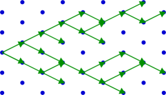
$t\to$

Figure 7: Directed percolation process (left) and critical DP cluster (right).

In fact, the field theory action should govern the scaling properties of generic continuous nonequilibrium phase transitions from active to inactive, absorbing states, namely for an order parameter with Markovian stochastic dynamics that is decoupled from any other slow variable, and in the absence of quenched randomness JanDP ; Grassb . This DP conjecture follows from the following phenomenological approach JanTau to simple epidemic processes (SEP), or epidemics with recovery Murray :

1. A ‘susceptible’ medium becomes locally ‘infected’, depending on the density $n$ of neighboring ‘sick’ individuals. The infected regions recover after a brief time interval.

2. The state $n=0$ is absorbing. It describes the extinction of the ‘disease’.

3. The disease spreads out diffusively via the short-range infection 1. of neighboring susceptible regions.

4. Microscopic fast degrees of freedom are incorporated as local noise or stochastic forces that respect statement 2., i.e., the noise alone cannot regenerate the disease.

These ingredients are captured by the coarse-grained mesoscopic Langevin equation $\partial_{t}\,n=D\left(\vec{\nabla}^{2}-R[n]\right)n+\zeta$ with a reaction functional $R[n]$, and s stochastic noise correlator of the form $L[n]=n\,N[n]$. Near the extinction threshold, we may expand $R[n]=r+u\,n\,+\ldots$, $N[n]=v+\ldots$, and higher-order terms turn out to be irrelevant in the RG sense. Upon rescaling, we recover the Reggeon field theory action (195) for DP as the corresponding response functional (34).

We now proceed to an explicit evaluation of the DP critical exponents to one-loop order, closely following the recipes given in Secs. 1.3–1.5. The lowest-order fluctuation contribution to the two-point vertex function $\Gamma^{(1,1)}(\vec{q},\omega)$ (propagator self-energy) is depicted in Fig. 8(a).

Figure 8: DP renormalisation: one-loop diagrams for the vertex functions (a) $\Gamma^{(1,1)}$ (propagator self-energy), and (b) $\Gamma^{(1,2)}=-\Gamma^{(2,1)}$ (nonlinear vertices).

The Feynman rules of Sec. 1.3 yield the corresponding analytic expression

$$\Gamma^{(1,1)}(\vec{q},\omega)={\rm i}\omega+D\,(r+\vec{q}^{2})+\frac{u^{2}}{D}\int_{k}\ \frac{1}{{\rm i}\omega/2D+r+\vec{q}^{2}/4+\vec{k}^{2}}\ .$$ (198)

The criticality condition $\Gamma^{(1,1)}(0,0)=0$ at $r=r_{c}$ provides us with the fluctuation-induced shift of the percolation threshold

$$r_{c}=-\frac{u^{2}}{D^{2}}\int_{k}^{\Lambda}\frac{1}{r_{c}+\vec{k}^{2}}+O(u^{4})\ .$$ (199)

Inserting $\tau=r-r_{c}$ into Eq. (198), we then find to this order

$$\Gamma^{(1,1)}(\vec{q},\omega)={\rm i}\omega+D\,(\tau+\vec{q}^{2})-\frac{u^{2}}{D}\int_{k}\frac{{\rm i}\omega/2D+\tau+\vec{q}^{2}/4}{\vec{k}^{2}\left({\rm i}\omega/2D+\tau+\vec{q}^{2}/4+\vec{k}^{2}\right)}\ ,$$ (200)

and the diagram in Fig. 8(b) for the three-point vertex functions, evaluated at zero external wavevectors and frequencies, gives

$$\Gamma^{(1,2)}(\{{\underline{0}}\})=-\Gamma^{(2,1)}(\{{\underline{0}}\})=-2u\left(1-\frac{2u^{2}}{D^{2}}\int_{k}\frac{1}{\left(\tau+\vec{k}^{2}\right)^{2}}\right)\ .$$ (201)

For the renormalisation factors, we use again the conventions (56) and (58), but with

$$u_{R}=Z_{u}\,u\,A_{d}^{1/2}\,\mu^{(d-4)/2}\ .$$ (202)

Because of rapidity inversion invariance, $Z_{\widetilde{S}}=Z_{S}$. With Eq. (53) the derivatives of $\Gamma^{(1,1)}$ with respect to $\omega$, $\vec{q}^{2}$, and $\tau$, as well as the one-loop result for $\Gamma^{(1,2)}$ in Eq. (201), all evaluated at the normalisation point $\tau_{R}=1$, provide us with the $Z$ factors

$$Z_{S}=1-\frac{u^{2}}{2D^{2}}\,\frac{A_{d}\,\mu^{-\epsilon}}{\epsilon}\ ,\quad Z_{D}=1+\frac{u^{2}}{4D^{2}}\,\frac{A_{d}\,\mu^{-\epsilon}}{\epsilon}\ ,$$

$$Z_{\tau}=1-\frac{3u^{2}}{4D^{2}}\,\frac{A_{d}\,\mu^{-\epsilon}}{\epsilon}\ ,\quad Z_{u}=1-\frac{5u^{2}}{4D^{2}}\,\frac{A_{d}\,\mu^{-\epsilon}}{\epsilon}\ .$$ (203)

From these we infer the RG flow functions

$$\gamma_{S}=v_{R}/2\ ,\quad\gamma_{D}=-v_{R}/4\ ,\quad\gamma_{\tau}=-2+3v_{R}/4\ ,$$ (204)

with the renormalised effective coupling

$$v_{R}=\frac{Z_{u}^{2}}{Z_{D}^{2}}\,\frac{u^{2}}{D^{2}}\,A_{d}\,\mu^{d-4}\ ,$$ (205)

whose RG beta function is to this order

$$\beta_{v}=v_{R}\left[-\epsilon+3v_{R}+O(v_{R}^{2})\right]\ .$$ (206)

For $d>d_{c}=4$, the Gaussian fixed point $v_{0}^{*}=0$ is stable, and we recover the mean-field critical exponents. For $\epsilon=4-d>0$, we find the nontrivial IR-stable RG fixed point

$$v^{*}=\epsilon/3+O(\epsilon^{2})\ .$$ (207)

Setting up and solving the RG equation (65) for the vertex function proceeds just as in Sec. 1.5. With the identifications (83) (with $a=0$) we thus obtain the DP critical exponents to first order in $\epsilon$,

$$\eta=-\frac{\epsilon}{6}+O(\epsilon^{2})\ ,\quad\frac{1}{\nu}=2-\frac{\epsilon}{4}+O(\epsilon^{2})\ ,\quad z=2-\frac{\epsilon}{12}+O(\epsilon^{2})\ .$$ (208)

In the vicinity of $v^{*}$, the solution of the RG equation for the order parameter reads, recalling that $[S]=\mu^{d/2}$,

$$\left\langle S_{R}(\tau_{R},t)\right\rangle\approx\mu^{d/2}\,\ell^{(d-\gamma_{S}^{*})/2}\,{\hat{S}}\left(\tau_{R}\,\ell^{\gamma_{\tau}^{*}},v_{R}^{*},D_{R}\,\mu^{2}\,\ell^{2+\gamma_{D}^{*}}\,t\right)\ ,$$ (209)

which leads to the following scaling relations and explicit exponent values,

$$\beta=\frac{\nu(d+\eta)}{2}=1-\frac{\epsilon}{6}+O(\epsilon^{2})\ ,\quad\alpha=\frac{\beta}{z\,\nu}=1-\frac{\epsilon}{4}+O(\epsilon^{2})\ .$$ (210)

Table 2: Comparison of the DP critical exponent values from Monte Carlo simulations with the results from the $\epsilon$ expansion.

Scaling exponent	$\ d=1$	$\ d=2$	$\ d=4-\epsilon$
$\xi\sim|\tau|^{-\nu}$	$\ \nu\approx 1.100$	$\ \nu\approx 0.735$	$\ \nu=1/2+\epsilon/16+O(\epsilon^{2})$
$t_{c}\sim\xi^{z}\sim|\tau|^{-z\nu}$	$\ z\approx 1.576$	$\ z\approx 1.73$	$\ z=2-\epsilon/12+O(\epsilon^{2})$
$a_{\infty}\sim|\tau|^{\beta}$	$\ \beta\approx 0.2765$	$\ \beta\approx 0.584$	$\ \beta=1-\epsilon/6+O(\epsilon^{2})$
$a_{c}(t)\sim t^{-\alpha}$	$\ \alpha\approx 0.160$	$\ \alpha\approx 0.46$	$\ \alpha=1-\epsilon/4+O(\epsilon^{2})$

The scaling exponents for critical directed percolation are known analytically for a plethora of physical quantities (but the reader should beware that various different conventions are used in the literature); for the two-loop results to order $\epsilon^{2}$ in the perturbative dimensional expansion, see Ref. JanTau . In Table 2, we compare the $O(\epsilon)$ values with the results from Monte Carlo computer simulations, which allow the DP critical exponents to be measured to high precision (for recent overviews on simulation results for DP and other absorbing state phase transitions, see Refs. Haye ; Odor ). Yet unfortunately, there are to date hardly any real experiments that would confirm the DP conjecture JanDP ; Grassb and actually measure the scaling exponents for this prominent nonequilibrium universality class.

2.6 Dynamic isotropic percolation and multi-species variants

An interesting variant of active to absorbing state phase transitions emerges when we modify the SEP rules (1) and (2) in Sec.2.5 to

1. The susceptible medium becomes infected, depending on the densities $n$ and $m$ of sick individuals and the ‘debris’, respectively. After a brief time interval, the sick individuals decay into immune debris, which ultimately stops the disease locally by exhausting the supply of susceptible regions.

2. The states with $n=0$ and any spatial distribution of $m$ are absorbing, and describe the extinction of the disease.

Here, the debris is given by the accumulated decay products,

$$m(\vec{x},t)=\kappa\int_{-\infty}^{t}n(\vec{x},t^{\prime})\,\mathrm{d}t^{\prime}\ .$$ (211)

After rescaling, this general epidemic process (GEP) or epidemic with removal Murray is described in terms of the mesoscopic Langevin equation GraPer

$$\frac{\partial S(\vec{x},t)}{\partial t}=-D\left(r-\vec{\nabla}^{2}\right)S(\vec{x},t)-D\,u\,S(\vec{x},t)\int_{-\infty}^{t}S(\vec{x},t^{\prime})\,Dt^{\prime}+\zeta(\vec{x},t)\ ,$$ (212)

with noise correlator (197). The associated response functional reads JanPer ; CarGra

$${\cal A}[{\widetilde{S}},S]=\int\!\mathrm{d}^{d}x\!\int\!\mathrm{d}t\,\biggl{[}{\widetilde{S}}\left(\frac{\partial}{\partial t}+D\left(r-\vec{\nabla}^{2}\right)\right)S-u\,{\widetilde{S}}^{2}\,S+D\,u\,S\int^{t}S(t^{\prime})\biggr{]}\ .$$ (213)

For the field theory thus defined, one may take the quasistatic limit by introducing the fields

$${\tilde{\varphi}}(\vec{x})={\widetilde{S}}(\vec{x},t\to\infty)\ ,\quad\varphi(\vec{x})=D\int_{-\infty}^{\infty}S(\vec{x},t^{\prime})\,\mathrm{d}t^{\prime}\ .$$ (214)

For $t\to\infty$, the action (213) thus becomes

$${\cal A}_{\rm qst}[{\tilde{\varphi}},\varphi]=\int\!\mathrm{d}^{d}x\,{\tilde{\varphi}}\Bigl{[}r-\vec{\nabla}^{2}-u\left({\tilde{\varphi}}-\varphi\right)\Bigr{]}\varphi\ ,$$ (215)

which is known to describe the critical exponents of isotropic percolation BenCar . An isotropic percolation cluster is shown in Fig. 9, to be contrasted with the anisotropic scaling evident in Fig. 7(b). The upper critical dimension of isotropic percolation is $d_{c}=6$, and an explicit calculation, with the diagrams of Fig. 8, but involving the static propagators $G_{0}(\vec{q})=1/(r+\vec{q}^{2})$, yields the following critical exponents for isotropic percolation, to first order in $\epsilon=6-d$,

$$\eta=-\frac{\epsilon}{21}+O(\epsilon^{2})\ ,\quad\frac{1}{\nu}=2-\frac{5\,\epsilon}{21}+O(\epsilon^{2})\ ,\quad\beta=1-\frac{\epsilon}{7}+O(\epsilon^{2})\ .$$ (216)

Figure 9: Isotropic percolation cluster.

In order to calculate the dynamic critical exponent for this dynamic isotropic percolation (dIP) universality class, we must return to the full action (213). Once again, with the diagrams of Fig. 8, but now involving a temporally nonlocal three-point vertex, one then arrives at

$$z=2-\frac{\epsilon}{6}+O(\epsilon^{2})\ .$$ (217)

For a variety of two-loop results, the reader is referred to Ref. JanTau . It is also possible to describe the crossover from isotropic to directed percolation within this field-theoretic framework FreTauSch ; JanSte .

Let us next consider multi-species variants of directed percolation processes, which can be obtained in the particle language by coupling the DP reactions $A_{i}\to\emptyset$, $A_{i}\rightleftharpoons A_{i}+A_{i}$ via processes of the form $A_{i}\rightleftharpoons A_{j}+A_{j}$ (with $j\not=i$); or directly by the corresponding generalisation within the Langevin representation with $\langle\zeta_{i}(\vec{x},t)\rangle=0$,

$$\frac{\partial S_{i}}{\partial t}=D_{i}\left(\vec{\nabla}^{2}-R_{i}[S_{i}]\right)S_{i}+\zeta_{i}\ ,\quad R_{i}[S_{i}]=r_{i}+\sum_{j}g_{ij}\,S_{j}+\ldots\ ,$$ (218)

$$\left\langle\zeta_{i}(\vec{x},t)\zeta_{j}(\vec{x}^{\prime},t^{\prime})\right\rangle=2S_{i}N_{i}[S_{i}]\,\delta(\vec{x}-\vec{x}^{\prime})\,\delta(t-t^{\prime})\,\delta_{ij}\,,\ N_{i}[S_{i}]=u_{i}+\ldots\qquad\$$ (219)

The ensuing renormalisation factors turn out to be precisely as for single-species DP, and consequently the generical critical behaviour even in such multi-species systems is governed by the DP universality class Hannes . For example, the predator extinction threshold for the stochastic Lotka–Volterra system mentioned in Sec. 2.1 is characterised by the DP exponents as well MoGeTa . But these reactions also generate $A_{i}\to A_{j}$, causing additional terms $\sum_{j\not=i}g_{j}\,S_{j}$ in Eqs. (218). Asymptotically, the inter-species couplings become unidirectional, which allows for the appearance of special multicritical points when several $r_{i}=0$ simultaneously TauHowHin . This leads to a hierarchy of order parameter exponents $\beta_{k}$ on the $k$th level of a unidirectional cascade, with

$$\beta_{1}=1-\frac{\epsilon}{6}+O(\epsilon^{2})\ ,\quad\beta_{2}=\frac{1}{2}-\frac{13\,\epsilon}{96}+O(\epsilon^{2})\ ,\ldots,\ \beta_{k}=\frac{1}{2^{k}}-O(\epsilon)\ ;$$ (220)

for the associated crossover exponent, one can show $\Phi=1$ to all orders Hannes . Quite analogous features emerge for multi-species dIP processes Hannes ; JanTau .

2.7 Concluding remarks

In these lecture notes, I have described how stochastic processes can be mapped onto field theory representations, starting either from a mesoscopic Langevin equation for the coarse-grained densities of the relevant order parameter fields and conserved quantities, or from a more microsopic master equation for interacting particle systems. The dynamic renormalisation group method can then be employed to study and characterise the universal scaling behaviour near continuous phase transitions both in and far from thermal equilibrium, and for systems that generically display scale-invariant features. While the critical dynamics near equilibrium phase transitions has been thoroughly investigated experimentally in the past three decades, regrettably such direct experimental verification of the by now considerable amount of theoretical work on nonequilibrium systems is largely amiss. In this respect, applications of the expertise gained in the nonequilibrium statistical mechanics of complex cooperative behaviour to biological systems might prove fruitful and constitutes a promising venture. One must bear in mind, however, that nonuniversal features are often crucial for the relevant questions in biology.

In part, the lack of clearcut experimental evidence may be due to the fact that asymptotic universal properties are perhaps less prominent in accessible nonequilibrium systems, owing to long crossover times. Yet fluctuations do tend to play a more important role in systems that are driven away from thermal equilibrium, and the concept of universality classes, despite the undoubtedly much increased richness in dynamical systems, should still be useful. For example, we have seen that the directed percolation universality class quite generically describes the critical properties of phase transitions from active to inactive, absorbing states, which abound in nature. The few exceptions to this rule either require the coupling to another conserved mode KrSS ; vWOeHi ; the presence, on a mesoscopic level, of additional symmetries that preclude the spontaneous decay $A\to\emptyset$ as in the so-called parity-conserving (PC) universality class, represented by branching and annihilating random walks $A\to(n+1)\,A$ with $n$ even, and $A+A\to\emptyset$ CarTau (for recent developments based on nonperturbative RG approaches, see Ref. CanChDel ); or the absence of any first-order reactions, as in the (by now rather notorious) pair contact process with diffusion (PCPD) HenHin , which has so far eluded a successful field-theoretic treatment JaWiDeTa . A possible explanation for the fact that DP exponents have not been measured ubiquitously (yet) could be the instability towards quenched disorder in the reaction rates JansDD .

In reaction–diffusion systems, a complete classification of the scaling properties in multi-species systems remains incomplete, aside from pair annihilation and DP-like processes, and still constitutes a quite formidable program (for a recent overview over the present situation from a field-theoretic viewpoint, see Ref. TauHowLee ). This is even more evident for nonequilibrium systems in general, even when maintained in driven steady states. Field-theoretic methods and the dynamic renormalisation group represent powerful tools that I believe will continue to crucially complement exact solutions (usually of one-dimensional models), other approximative approaches, and computer simulations, in our quest to further elucidate the intriguing cooperative behaviour of strongly interacting and fluctuating many-particle systems.

Acknowledgements

This work has been supported in part by the U.S. National Science Foundation through grant NSF DMR-0308548. I am indebted to many colleagues, students, and friends, from and with whom I had the pleasure to learn and research the material presented here; specifically I would like to mention Vamsi Akkineni, Michael Bulenda, John Cardy, Olivier Deloubrière, Daniel Fisher, Reinhard Folk, Erwin Frey, Ivan Georgiev, Yadin Goldschmidt, Peter Grassberger, Henk Hilhorst, Haye Hinrichsen, Martin Howard, Terry Hwa, Hannes Janssen, Bernhard Kaufmann, Mauro Mobilia, David Nelson, Beth Reid, Zoltán Rácz, Jaime Santos, Beate Schmittmann, Franz Schwabl, Steffen Trimper, Ben Vollmayr-Lee, Mark Washenberger, Fred van Wijland, and Royce Zia. Lastly, I would like to thank the organisers of the very enjoyable Luxembourg Summer School on Ageing and the Glass Transition for their kind invitation, and my colleagues at the Laboratoire de Physique Théorique, Université de Paris-Sud Orsay, France and at the Rudolf Peierls Centre for Theoretical Physics, University of Oxford, U.K., where these lecture notes were conceived and written, for their warm hospitality.

References

- (1) P. Ramond: Field theory — a modern primer, (Benjamin/Cummings, Reading 1981)
- (2) D.J. Amit: Field theory, the renormalization group, and critical phenomena (World Scientific, Singapore 1984)
- (3) C. Itzykson and J.M. Drouffe: Statistical field theory (Cambridge University Press, Cambridge 1989)
- (4) M. Le Bellac: Quantum and statistical field theory, (Oxford University Press, Oxford 1991)
- (5) J. Zinn-Justin: Quantum field theory and critical phenomena (Clarendon Press, Oxford 1993)
- (6) J. Cardy: Scaling and renormalization in statistical physics (Cambridge University Press, Cambridge 1996)
- (7) P.C. Hohenberg and B.I. Halperin: Rev. Mod. Phys. 49, 435 (1977)
- (8) H.K. Janssen: Field-theoretic methods applied to critical dynamics. In: Dynamical critical phenomena and related topics, Lecture Notes in Physics, vol. 104, ed by C.P. Enz (Springer, Heidelberg 1979), pp. 26-47
- (9) R. Bausch, H.K. Janssen, and H. Wagner: Z. Phys. B 24, 113 (1976)
- (10) J.L. Cardy: Renormalisation group approach to reaction-diffusion problems. In: Proceedings of Mathematical Beauty of Physics, ed by J.-B. Zuber, Adv. Ser. in Math. Phys. 24, 113 (1997)
- (11) D.C. Mattis and M.L. Glasser: Rev. Mod. Phys. 70, 979 (1998)
- (12) U.C. Täuber, M.J. Howard, and B.P. Vollmayr-Lee: J. Phys. A: Math. Gen. 38, R79 (2005)
-
(13)
U.C. Täuber:
Critical dynamics: a field theory approach to equilibrium and
non-equilibrium scaling behavior, in preparation (to be published at
Cambridge University Press, Cambridge); for completed chapters, see:
http://www.phys.vt.edu/tauber/utaeuber.html - (14) R.A. Ferrell, N. Menyhàrd, H. Schmidt, F. Schwabl, and P. Szépfalusy: Phys. Rev. Lett. 18, 891 (1967); Ann. Phys. (NY) 47, 565 (1968)
- (15) B.I. Halperin and P.C. Hohenberg: Phys. Rev. 177, 952 (1969)
- (16) B.I. Halperin, P.C. Hohenberg, and S.-k. Ma: Phys. Rev. Lett. 29, 1548 (1972)
- (17) C. De Dominicis, E. Brézin, and J. Zinn-Justin: Phys. Rev. B 12, 4945 (1975)
- (18) H.K. Janssen: Z. Phys. B 23, 377 (1976)
- (19) C. De Dominicis: J. Phys. (France) Colloq. 37, C2247 (1976)
- (20) P.C. Martin, E.D. Siggia, and H.A. Rose: Phys. Rev. A 8, 423 (1973)
- (21) H. Wagner: Z. Phys. 195, 273 (1966)
- (22) N.D. Mermin and H. Wagner: Phys. Rev. Lett. 17, 1133 (1966)
- (23) P.C. Hohenberg: Phys. Rev. 158, 383 (1967)
- (24) P.M. Chaikin and T.C. Lubensky: Principles of condensed matter physics, (Cambridge University Press, Cambridge 1995)
- (25) S.-k. Ma and G.F. Mazenko: Phys. Rev. Lett. 33, 1383 (1974); Phys. Rev. B 11, 4077 (1975)
- (26) E. Frey and F. Schwabl: Adv. Phys. 43, 577 (1994)
- (27) H.K. Janssen, B. Schaub, and B. Schmittmann: Z. Phys. B 73, 539 (1989)
- (28) H.K. Janssen: On the renormalized field theory of nonlinear critical relaxation. In: From phase transitions to chaos, ed by G. Györgyi, I. Kondor, L. Sasvári, and T. Tél (World Scientific, Singapore 1992), pp. 68-91.
- (29) P. Calabrese and A. Gambassi: Phys. Rev. E 66, 066101 (2002); J. Phys. A: Math. Gen. 38, R133 (2005)
- (30) A. Gambassi: In: Proceedings of the International Summer School “Ageing and the Glass Transition”, to appear in J. Phys. A: Math. Gen. (2006)
- (31) H.W. Diehl: In: Phase Transitions and Critical Phenomena, vol. 10, ed by C. Domb and J.L. Lebowitz (Academic Press, London 1986)
- (32) K. Oerding and H.K. Janssen: J. Phys. A: Math. Gen. 26, 5295 (1993)
- (33) U.C. Täuber, V.K. Akkineni, and J.E. Santos: Phys. Rev. Lett. 88, 045702 (2002)
- (34) F. Haake, M. Lewenstein, and M. Wilkens: Z. Phys. B 55, 211 (1984)
- (35) G. Grinstein, C. Jayaprakash, and Y. He: Phys. Rev. Lett. 55, 2527 (1985)
- (36) K.E. Bassler and B. Schmittmann: Phys. Rev. Lett. 73, 3343 (1994)
- (37) U.C. Täuber and Z. Rácz: Phys. Rev. E 55, 4120 (1997)
- (38) U.C. Täuber, J.E. Santos, and Z. Rácz: Eur. Phys. J. B 7, 309 (1999)
- (39) B. Schmittmann and R.K.P. Zia: Phys. Rev. Lett. 66, 357 (1991)
- (40) B. Schmittmann: Europhys. Lett. 24, 109 (1993)
- (41) K.E. Bassler and Z. Rácz: Phys. Rev. Lett. 73, 1320 (1994); Phys. Rev. E 52, R9 (1995)
- (42) B. Schmittmann and R.K.P. Zia: Statistical mechanics of driven diffusive systems. In: Phase Transitions and Critical Phenomena, vol. 17, ed by C. Domb and J.L. Lebowitz (Academic Press, London 1995)
- (43) H.K. Janssen and B. Schmittmann: Z. Phys. B 63, 517 (1986)
- (44) K.-t. Leung and J.L. Cardy: J. Stat. Phys. 44, 567 (1986)
- (45) D. Forster, D.R. Nelson, and M.J. Stephen: Phys. Rev. A 16, 732 (1977)
- (46) J.D. Murray: Mathematical Biology, vols. I/II (Springer, New York, 3rd ed 2002)
- (47) M. Mobilia, I.T. Georgiev, and U.C. Täuber: e-print q-bio.PE/0508043 (2005)
- (48) M. Doi: J. Phys. A: Math. Gen. 9, 1465 & 1479 (1976)
- (49) P. Grassberger and M. Scheunert: Fortschr. Phys. 28, 547 (1980)
- (50) L. Peliti: J. Phys. (Paris) 46, 1469 (1985)
- (51) F.C. Alcaraz, M. Droz, M. Henkel, and V. Rittenberg: Ann. Phys. (NY) 230, 250 (1994)
- (52) M. Henkel, E. Orlandini, and J. Santos: Ann. Phys. (NY) 259, 163 (1997)
- (53) G.M. Schütz: In: Phase Transitions and Critical Phenomena, vol. 19, ed by C. Domb and J.L. Lebowitz (Academic Press, London 2001)
- (54) R. Stinchcombe: Adv. Phys. 50, 431 (2001)
- (55) F. van Wijland: Phys. Rev. E 63, 022101 (2001)
- (56) J.W. Negele and H. Orland: Quantum many-particle systems (Addison-Wesley, Redwood City 1988)
- (57) L. Peliti: J. Phys. A: Math. Gen. 19, L365 (1986)
- (58) H.K. Janssen: J. Stat. Phys. 103, 801 (2001)
- (59) B.P. Lee: J. Phys. A: Math. Gen. 27, 2633 (1994)
- (60) B.P. Lee and J. Cardy: Phys. Rev. E 50, R3287 (1994)
- (61) D. Toussaint and F. Wilczek: J. Chem. Phys. 78, 2642 (1983)
- (62) B.P. Lee and J. Cardy: J. Stat. Phys. 80, 971 (1995)
- (63) O. Deloubrière, H.J. Hilhorst, and U.C. Täuber: Phys. Rev. Lett. 89, 250601 (2002); H.J. Hilhorst, O. Deloubrière, M.J. Washenberger, and U.C. Täuber: J. Phys. A: Math. Gen. 37, 7063 (2004)
- (64) H.J. Hilhorst, M.J. Washenberger, and U.C. Täuber: J. Stat. Mech. P10002 (2004)
- (65) M. Moshe: Phys. Rep. C 37, 255 (1978)
- (66) P. Grassberger and K. Sundermeyer: Phys. Lett. B 77, 220 (1978)
- (67) P. Grassberger and A. De La Torre: Ann. Phys. (NY) 122, 373 (1979)
- (68) H.K. Janssen and U.C. Täuber: Ann. Phys. (NY) 315, 147 (2005)
- (69) S.P. Obukhov: Physica A 101, 145 (1980)
- (70) J.L. Cardy and R.L.Sugar: J. Phys. A: Math. Gen. 13, L423 (1980)
- (71) H.K. Janssen: Z. Phys. B 42, 151 (1981)
- (72) W. Kinzel: In: Percolation structures and processes, ed by G. Deutsch, R. Zallen, and J. Adler (Hilger, Bristol 1983)
- (73) P. Grassberger, Z. Phys. B 47, 365 (1982)
- (74) H. Hinrichsen: Adv. Phys. 49, 815 (2001)
- (75) G. Ódor: Rev. Mod. Phys. 76, 663 (2004)
- (76) P. Grassberger: Math. Biosc. 63, 157 (1983)
- (77) H.K. Janssen: Z. Phys. B 58, 311 (1985)
- (78) J.L. Cardy and P. Grassberger: J. Phys. A: Math. Gen. 18, L267 (1985)
- (79) J. Benzoni and J.L. Cardy: J. Phys. A: Math. Gen. 17, 179 (1984)
- (80) E. Frey, U.C. Täuber, and F. Schwabl: Europhys. Lett. 26, 413 (1994); Phys. Rev. E 49, 5058 (1994)
- (81) H.K. Janssen and O. Stenull: Phys. Rev. E 62, 3173 (2000)
- (82) U.C. Täuber, M.J. Howard, and H. Hinrichsen: Phys. Rev. Lett. 80, 2165 (1998); Y.Y. Goldschmidt, H. Hinrichsen, M.J. Howard, and U.C. Täuber: Phys. Rev. E 59, 6381 (1999)
- (83) R. Kree, B. Schaub, and B. Schmittmann: Phys. Rev. A 39, 2214 (1989)
- (84) F. van Wijland, K. Oerding, and H. Hilhorst: Physica A 251, 179 (1998); K. Oerding, F. van Wijland, J.P. Leroy, and H. Hilhorst: J. Stat. Phys. 99, 1365 (2000)
- (85) J. Cardy and U.C. Täuber: Phys. Rev. Lett. 77, 4780 (1996); J. Stat. Phys. 90, 1 (1998)
- (86) L. Canet, H. Chaté, and B. Delamotte: Phys. Rev. Lett. 92, 255703 (2004); L. Canet, H. Chaté, B. Delamotte, I. Dornic, and M.A. Muñoz: e-print cond-mat/0505170 (2005)
- (87) M. Henkel and H. Hinrichsen: J. Phys. A: Math. Gen. 37, R117 (2004)
- (88) H.K. Janssen, F. van Wijland, O. Deloubrière, and U.C. Täuber: Phys. Rev. E 70, 056114 (2004)
- (89) H.K. Janssen: Phys. Rev. E 55, 6253 (1997)