Real Space Hartree-Fock Configuration Interaction Method For Complex Lateral Quantum Dot Molecules

Abstract

We present unrestricted Hartree Fock method coupled with configuration interaction (CI) method (URHF-CI) suitable for the calculation of ground and excited states of large number of electrons localized by complex gate potentials in quasi-two-dimensional quantum dot molecules. The method employs real space finite difference method, incorporating strong magnetic field, for the calculating of single particle states. The Hartree-Fock method is employed for the calculation of direct and exchange interaction contribution to the ground state energy. The effects of correlations are included in energies and directly in the many-particle wavefunctions via configuration interaction (CI) method using a limited set of excitations above the Fermi level. The URHF-CI method and its performance are illustrated on the example of ten electrons confined in a two-dimensional quantum dot molecule.

I Introduction

There is currently interest in localizing electrons in quantum dots and utilizing their spin for quantum information processing qinfo ; brum ; Loss-DiVincenzo . Alternatively, we can view such devices as highly tunable quantum dot molecules, with large numbers of electrons or qubits, with gates and magnetic field used to perform quantum operations. Even with a relatively small number of bits, to understand working of such devices one needs a computational tool suitable for the calculation of wavefunctions of at least tens of electrons confined by complex gate potentials and in magnetic field. The wavefunctions must capture entanglement, or in condensed matter language, correlations. The configuration interaction (CI) method is a suitable candidate modified here for the problem of quantum dot molecules. In the configuration interaction (CI) method the Hamiltonian of an interacting system is calculated in the basis of a finite number of many-electron configurations and diagonalized exactly. Exact diagonalization (ED) has been an important tool in the context of quantum chemistry of atoms and molecules Szabo_book . In condensed matter physics ED has been used to investigate the electronic and optical properties of artificial atoms and molecules in quantum dots (QDs) jacak98 ; maksym90 ; merkt91 ; pfannkuche93 ; hawrylak93 ; yang93 ; hawrylak93b ; palacios94 ; wojs95 ; oaknin96 ; wojs96 ; maksym96 ; hawrylak96 ; wojs97 ; wojs97b ; eto97 ; eto97b ; maksym98 ; imamura98 ; imamura98b ; hawrylak99 ; creffield99 ; bruce00 ; reimann00 ; mikhailov02 ; palacios ; KRKM ; HuDasSarma ; WKH ; WKH2 ; Rontani ; RaminWojtekPawel and finite size quantum Hall systems. Yoshioka ; HaldaneRezayi ; RezayiHaldane ; FanoOrtolaniColombo The direct access to electron correlations in the many-particle wave functions calculated by CI makes CI useful for the purpose of quantitative description of the electron entanglement in the context of solid state quantum information architectures. The drawback of the method is its slow convergence and applicability to a small number of electrons. While mean-field theories such as Hartree-Fock (HF) yannouleas99 ; reusch01 , and density-functional theory (DFT) koskinen97 ; austing99 ; hirose99 ; steffens99 ; wensauer00 ; wensauer01 ; Zhuang can be applied to large electron numbers, they neglect electron correlations, or entanglement, in the wavefunction.

To include electron correlations explicitly in the many-particle wavefunctions one may follow quantum chemistry methods which start with HF or DFT calculations of effective single particle orbitals, and use them in the construction of a finite number of many-electron configurations as input in configuration interaction calculations Szabo_book . These ideas have been already explored for the calculation of electronic properties of quantum dots with large electron numbersWKH and quantum dot molecules.HuDasSarma ; RaminWojtekPawel

The objective of this work is to present an efficient HF-CI method: (a) based on real space calculations of single particle states and hence suitable for complex quantum dot potentials, (b) combining complex potentials with strong magnetic field, and (c) capable of treating correlations (entanglement) in electron wavefunction for large number of electrons. The URHF-CI method and its performance are illustrated on the example of ten electron confined in a two-dimensional quantum dot molecule.

The paper is organized as follows: In section II we present the Hamiltonian of electrons confined in the lateral gated quantum dot molecule. The calculation of the single particle spectrum, including the details of the implementation of the localized gauge, is presented in section III. In section IV our many electron approach, including the unrestricted Hartree-Fock approximation, is introduced. The central results of this study, the calculation of the ground state energy and excitation gap by configuration interaction method using unrestricted Hartree-Fock URHF-CI basis and non-interacting single particle SP-CI basis, are presented in section V. The paper is summarized in section VI.

II Hamiltonian

We consider $N$ electrons with effective mass $m^{*}$, moving on a plane $(x,y)$ defined by the GaAs/GaAlAs interface, with complicated confining potential $V(\vec{r})$ as a function of electron position $\vec{r}$, created by metallic gates on the surface of the heterostructure. The magnetic field, defined by vector potential $A$, is perpendicular to the 2D plane. The effective $N$-electron quantum dot molecule Hamiltonian in the presence of an external magnetic field can be written as:

$$H = \sum_{i=1}^{N}\left[\frac{1}{2m^{*}}\left(\frac{\hbar}{i}\vec{\nabla}_{i}+\frac{e}{c}A(\vec{r}_{i})\right)^{2}+V(x_{i},y_{i})\right]$$ (1)

$$+\frac{e^{2}}{2\epsilon}\sum_{i\neq j}\frac{1}{|\vec{r}_{i}-\vec{r}_{j}|},$$

where $e$ is electron charge, $c$ is velocity of light, and $\epsilon$ is the host semiconductor dielectric constant.The Zeeman splitting (very small for GaAs) is neglected here. The first term in Eq. (1) is the sum of single particle Hamiltonians and the second term is the Coulomb repulsion. The electron-electron repulsion is screened by the dielectric constant, which for GaAs is $\epsilon\approx 12.4$.

In what follows, we present the results in effective atomic units with length unit in effective Bohr radii $a^{*}_{0}=(\hbar^{2}/2m^{*})/(e^{2}/2\epsilon)$, and energy unit in effective Rydberg $Ry^{*}=e^{2}/(2\epsilon a^{*}_{0})$. Using material parameters for GaAs with $m^{*}\approx 0.067m_{0}$ ($m_{0}$ is the bare electron mass) $Ry^{*}=5.93meV$, and $a^{*}_{0}=9.79nm$.

III Single particle spectrum in a magnetic field

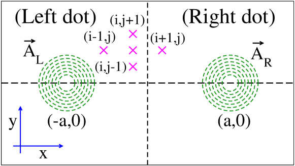
Figure 1: discrete points in left (L) and right (R) dot regions.

The single particle Schrödinger equation is given by

$$\left[\frac{1}{2m^{*}}\left(\frac{\hbar}{i}\vec{\nabla}+\frac{e}{c}A(\vec{r})\right)^{2}+V(\vec{r})\right]\tilde{\varphi}(\vec{r})=\varepsilon\tilde{\varphi}(\vec{r}),$$ (2)

where $A=(B/2)(-y,x)$ is the vector potential seen by electrons, $V(\vec{r})$ is the confining potential, and $B$ is the magnetic field. For a single quantum dot the potential is often well approximated by an analytical form $V(\vec{r})=1/2m\omega^{2}r^{2}$. For quantum dot molecules the potential will have several minima in which to localize electrons, and the most convenient way to solve the single particle problem is by discretizing the Schrödinger equation. As an example of a complicated molecular quantum dot potential we study a double Gaussian potential $V(x,y)=V_{L}~{}\exp[{-\frac{(x+a)^{2}+y^{2}}{\Delta^{2}}}]+V_{R}~{}\exp[{-\frac{(x-a)^{2}+y^{2}}{\Delta^{2}}}]+V_{p}\exp[{-\frac{x^{2}}{\Delta_{Px}^{2}}-\frac{y^{2}}{\Delta_{Py}^{2}}}]$, with $V_{L}$ and $V_{R}$ measuring the depth of the left and right dot, and $V_{p}$ controlling the height of the tunneling barrier. The centers of the two dots are separated by $2a$. To describe the typical coupled quantum dots we use the parameters $V_{L}=V_{R}=-10,a=2,\Delta=2.5$, and $\Delta_{Px}=0.3$, $\Delta_{Py}=2.5$, in effective atomic units. $V_{p}$ which controls the central potential barrier mimics the plunger gate strength and is varied between zero and $10Ry^{*}$, independent of the locations of the quantum dots.

The choice of gauge $A$ plays significant role in improving the numerical accuracy of single particle spectrum. We use a gauge field which is adopted to the geometry of the confining potential. For a double dot molecule with two minima, we divide the plane of coupled quantum dots into left and right domains, as shown in Fig. 1. In order to end up with a well defined left and right quantum dots with increasing barrier height, i.e. with dots with gauge centered in the origin, we define left (right) wavefunctions and Hamiltonians, and carry out gauge transformation on both Hamiltonians and wavefunctions. The resulting vector potentials localized in centers of each dot are $A_{L}=(B/2)(-y,x+a)$ for the left dot ( $x<0$ ), and $A_{R}=(B/2)(-y,x-a)$ for the right dot ($x>0$). Introducing corresponding wavefunctions in the left (right) dot $\tilde{\varphi}_{i,j}=\tilde{\varphi}^{L}_{i,j}\exp(+i\omega_{c}ay/4)$ ($\tilde{\varphi}_{i,j}=\tilde{\varphi}^{R}_{i,j}\exp(-i\omega_{c}ay/4)$) allows us to write an explicit form of the discrete form of Schrödinger equation. In the left-dot the Schrödinger equation can be obtained by expanding $\tilde{\varphi}^{L}$ around the point $(i,j)$

$$-\frac{1}{h^{2}}\left[\tilde{\varphi}^{L}_{i+1,j}+\tilde{\varphi}^{L}_{i-1,j}+\tilde{\varphi}^{L}_{i,j+1}+\tilde{\varphi}^{L}_{i,j-1}-4\tilde{\varphi}^{L}_{i,j}\right]$$

$$-i\frac{\hbar\omega_{c}}{4h}\left[(x_{i}+a)(\tilde{\varphi}^{L}_{i,j+1}-\tilde{\varphi}^{L}_{i,j-1})-y_{j}(\tilde{\varphi}^{L}_{i+1,j}-\tilde{\varphi}^{L}_{i-1,j})\right]$$

$$+\frac{(\hbar\omega_{c})^{2}}{16}\left[(x_{i}+a)^{2}+y_{j}^{2}\right]\tilde{\varphi}^{L}_{i,j}+V_{i,j}\tilde{\varphi}^{L}_{i,j}=\varepsilon\tilde{\varphi}^{L}_{i,j}$$ (3)

where $x_{i}=ih$, and $y_{j}=jh$, and $h$ is the grid spacing. A similar equation holds for the wavefunction in the right dot.

As it is illustrated in Fig. 1, adjacent to the inter-dot boundary, the point $(i,j)$ in L, is connected to the point $(i+1,j)$ in R, via Schrödinger equation. In this case $\tilde{\varphi}^{L}_{i+1,j}$ in Eq.(3) is already in the right dot and is not known and must be replaced by $\tilde{\varphi}^{R}_{i+1,j}\exp(-i\omega_{c}ay/2)$.

One should note that this separation of gauge fields into left and right leads to a uniform magnetic field $B=\nabla\times A$ in both half-planes, but it produces an artifical discontinuity in $B$ along $x=0$. To avoid this unphysical discontinuity, in finite difference method, the grids along the $x$-axis have been set slightly away from $x=0$ such that $x=0$-line has been excluded from the real space finite difference calculation.

The single particle spectrum $\tilde{\epsilon}_{j}$ and $\tilde{\varphi}_{j}$ is calculated accurately on a finite mesh of $N_{x}\times N_{y}$ ($102\times 51$ mesh points are used in what follows) using conjugated gradient methods. The magnetic field dependence of single particle spectrum calculated by this method, is shown in Fig. 2. At zero magnetic field Fig. 2 shows the formation of hybridized S, P, and D shells. In high magnetic field we observe the formation of shells of closely spaced pairs of levels (with opposite parity). In intermediate magnetic field states with opposite parity cross and states with the same parity anticross. The crossing of many levels at e.g. $\hbar\omega_{c}=1.4Ry^{*}$, marked with dashed line in Fig.2, leads to the most computationally challenging many-electron problem.

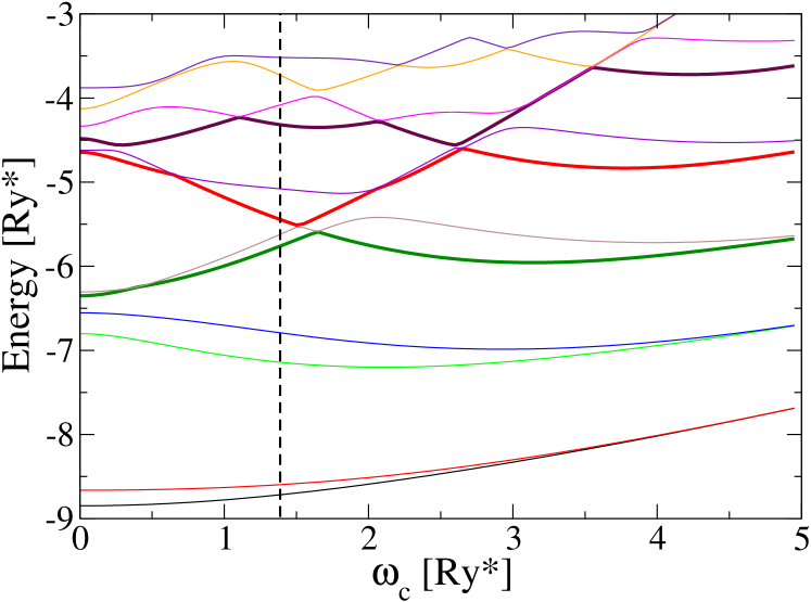
Figure 2: Double dot single particle spectrum vs. cyclotron energy. Several crossing between Landau levels is visible at $\hbar\omega_{c}=1.4Ry^{*}$.

IV Many electron spectrum

The single-particle (SP) states calculated in previous section can be used as a basis in configuration-interaction (CI) calculation. Denoting the creation (annihilation) operators for electron in non-interacting SP state $|\alpha\sigma\rangle$ by $\tilde{c}^{\dagger}_{\alpha\sigma}~{}(\tilde{c}_{\alpha\sigma})$, the Hamiltonian of an interacting system in second quantization can be written as

$$H = \sum_{\alpha}\sum_{\sigma}\tilde{\epsilon}_{\alpha}\tilde{c}^{\dagger}_{\alpha\sigma}\tilde{c}_{\alpha\sigma}$$ (4)

$$+\frac{1}{2}\sum_{\alpha\beta\gamma\mu}\sum_{\sigma\sigma^{\prime}}\tilde{V}_{\alpha\sigma,\beta\sigma^{\prime},\gamma\sigma^{\prime},\mu\sigma}\tilde{c}^{\dagger}_{\alpha\sigma}\tilde{c}^{\dagger}_{\beta\sigma^{\prime}}\tilde{c}_{\gamma\sigma^{\prime}}\tilde{c}_{\mu\sigma}$$

where the first term is the single particle Hamiltonian, and $\tilde{V}_{\alpha\sigma,\beta\sigma^{\prime},\mu\sigma^{\prime},\nu\sigma}=\int d\vec{r}\int d\vec{r^{\prime}}\tilde{\varphi}^{*}_{\alpha\sigma}(\vec{r})\tilde{\varphi}^{*}_{\beta\sigma^{\prime}}(\vec{r^{\prime}})\frac{e^{2}}{\epsilon|\vec{r}-\vec{r^{\prime}}|}\tilde{\varphi}_{\mu\sigma^{\prime}}(\vec{r^{\prime}})\tilde{\varphi}_{\nu\sigma}(\vec{r})$, is the two-body Coulomb matrix element.

Alternatively we may use the single particle states to first construct the Hartree-Fock orbitals. In this scheme electrons are treated as independent particles moving in a self-consistent HF field. Similar to single particle configuration-interaction (SP-CI) method, the HF orbitals can be used as a basis of the interacting Hamiltonian in second quantization, and subsequently in the CI calculation. In this method electron-electron interactions are included in two steps: direct and exchange interaction using Hartree-Fock approximation, and correlations using HF basis in the configuration interaction method.

IV.1 Unrestricted Hartree-Fock Approximation (URHFA)

Hartree-Fock approximation is a mean field approach to many body systems which accounts for the direct and exchange Coulomb interactions. Combining HFA with more sophisticated many body methods (such as CI) allows to isolate the effect introduced by correlations. The Hartree-Fock ground state (GS) of the electrons with given $S_{z}=(N_{\uparrow}-N_{\downarrow})/2$ is a single Slater determinant

$$|\Psi\rangle=\frac{1}{\sqrt{N}!}\sum_{P}(-1)^{P}\varphi_{1\sigma_{1}}(r_{P1})|\sigma_{1}\rangle\dots\varphi_{N\sigma_{N}}(r_{PN})|\sigma_{N}\rangle,$$ (5)

with $P$ the permutation operator. The HF orbitals $|\varphi_{i\sigma}\rangle$ which describe the state of a dressed quasi-particle in the quantum dot molecule can be determined by minimizing the HF energy $E_{HF}=\langle\Psi|H|\Psi\rangle$ with respect to $\varphi_{i\sigma}(r)$

$$\left\{\hat{T}+\int d^{2}r^{\prime}\sum_{\sigma^{\prime}}\sum_{j=1}^{N_{\sigma^{\prime}}}|\varphi_{j\sigma^{\prime}}(\vec{r}^{\prime})|^{2}V(|\vec{r}-\vec{r}^{\prime}|)\right\}\varphi_{i\sigma}(\vec{r})$$

$$-\sum_{\sigma^{\prime}}\sum_{j=1}^{N_{\sigma^{\prime}}}\varphi_{j\sigma}(\vec{r})\int d^{2}r^{\prime}\varphi^{*}_{j\sigma^{\prime}}(\vec{r}^{\prime})V(|\vec{r}-\vec{r}^{\prime}|)\varphi_{i\sigma^{\prime}}(\vec{r}^{\prime})\delta_{\sigma\sigma^{\prime}}$$

$$=\epsilon_{i\sigma}\varphi_{i\sigma}(\vec{r}).$$ (6)

$\hat{T}=\frac{1}{2m^{*}}(\frac{\hbar}{i}\vec{\nabla}+\frac{e}{c}A)^{2}$ is the non-interacting single particle Hamiltonian, and $V(r)=e^{2}/\epsilon r$ is the Coulomb interaction. This equation is a set of coupled equations, for spin up and spin down states. To find numerical solutions of the Hartree-Fock equations we expand the HF orbitals $|\varphi_{i\sigma}\rangle$ in terms of single particle states $|\tilde{\varphi}_{\alpha}\rangle$: $|\varphi_{i\sigma},\sigma\rangle=\sum_{\alpha=1}^{N_{l}}a^{(i)}_{\alpha\sigma}|\tilde{\varphi}_{\alpha},\sigma\rangle$. This transforms the HF equation, Eq.(6), to the self-consistent Pople-Nesbet equations Szabo_book :

$$\sum_{\gamma=1}^{N_{l}}\{\tilde{\epsilon}_{\mu}\delta_{\gamma\mu}+\sum_{\alpha,\beta=1}^{N_{l}}\tilde{V}_{\mu\alpha\beta\gamma}\sum_{\sigma^{\prime}}\sum_{j=1}^{N_{\sigma^{\prime}}}a^{*(j)}_{\alpha\sigma^{\prime}}a_{\beta\sigma^{\prime}}^{(j)}$$

$$-\tilde{V}_{\mu\alpha\gamma\beta}\sum_{\sigma^{\prime}}\sum_{j=1}^{N_{\sigma^{\prime}}}a^{*(j)}_{\alpha\sigma^{\prime}}a_{\beta\sigma^{\prime}}^{(j)}\delta_{\sigma,\sigma^{\prime}}\}a_{\gamma\sigma}^{(i)}=\epsilon_{i\sigma}~{}a_{\mu\sigma}^{(i)},$$ (7)

where $\tilde{V}_{\alpha\beta\mu\nu}$ are Coulomb matrix elements calculated using non-interacting single particle states.

This procedure results in $N_{l}$ HF states. The $N$-lowest energy states form a Slater determinant occupied by HF (quasi) electrons corresponding to HF ground state. The rest of orbitals with higher energies are outside of the HF Slater determinant (unoccupied states).

The calculated HF eigen-energies for the $N=10$ electrons with $S_{z}=0$ as a function of magnetic field are shown in Fig. 3. Comparing HF spectrum (Fig. 3) with the single particle spectrum (Fig. 2), one observes that a HF gap developed at the Fermi level, between the highest occupied molecular state, and the lowest unoccupied molecular state, and the Landau level crossing between single particle Landau levels has been shifted to lower magnetic fields.

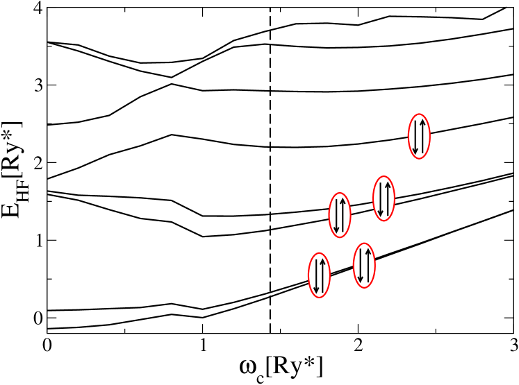
Figure 3: URHF eigen-energies vs. cyclotron energy for 10 electrons with $S_{z}=0$. The HF energy gap between HOMO (highest occupied molecular orbital), and LUMO (lowest unoccupied molecular orbital) is clearly visible. A comparison between SP-CI and URHF-CI calculation will be presented at $\hbar\omega_{c}=1.4Ry^{*}$, and it is shown by the dash line.

Fig. 4 illustrates the convergence of HF energy with respect to the number $N_{l}$ of single particle orbitals used in HF expansion.

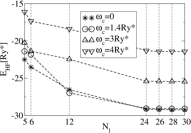
Figure 4: HFA ground state energy vs. number of single particle states participated in HF calculation ($N_{l}$) for 10 electrons.

In the following we study the effect of correlations by including quasielectron-quasihole excitations in the HF wave functions using CI method.

V Configuration-interaction method

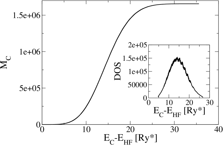
Figure 5: URHF electron-hole excitation energies $E_{C}=\langle\Psi_{M_{C}}|H|\Psi_{M_{C}}\rangle$ for $N_{s}=13$ corresponding to $N_{C}=1656369$ is plotted vs. $M_{C}$. Here $1\leq M_{C}\leq N_{C}$ is an integer number. $|\Psi_{M_{C}}\rangle$ is the Slater determinant of the configuration $M_{C}$th, formed by HF basis. $E_{C}=E_{HF}$ (the HF ground state) if $M_{C}=1$. The URHF density of states ($dM_{C}/dE_{C}$) is shown in inset. Its peak is below the HF energy mean value.

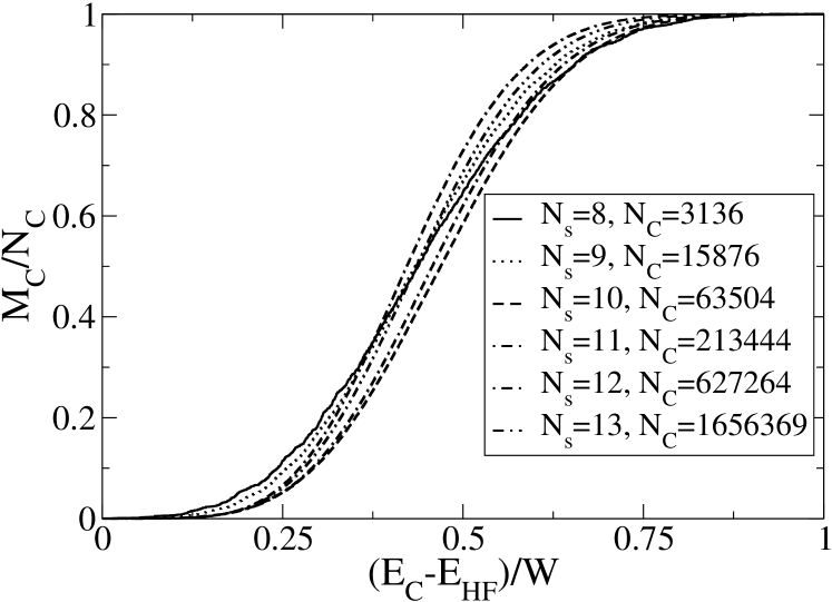
Figure 6: The URHF excitation energies $E_{C}$ corresponding to the $M_{C}$th diagonal matrix elements in $H$ (see Eq.LABEL:IR7), are shown for various configurations. Due to the finite band width $W$ of the HF spectrum, they approximately follow a universal functional form.

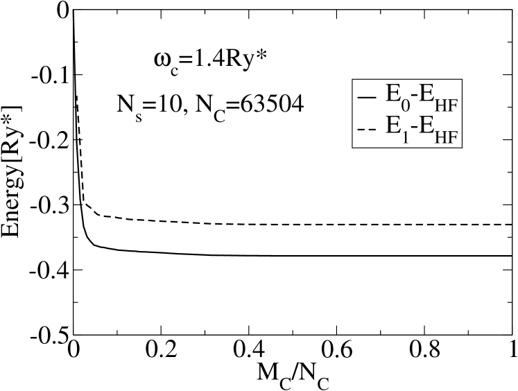
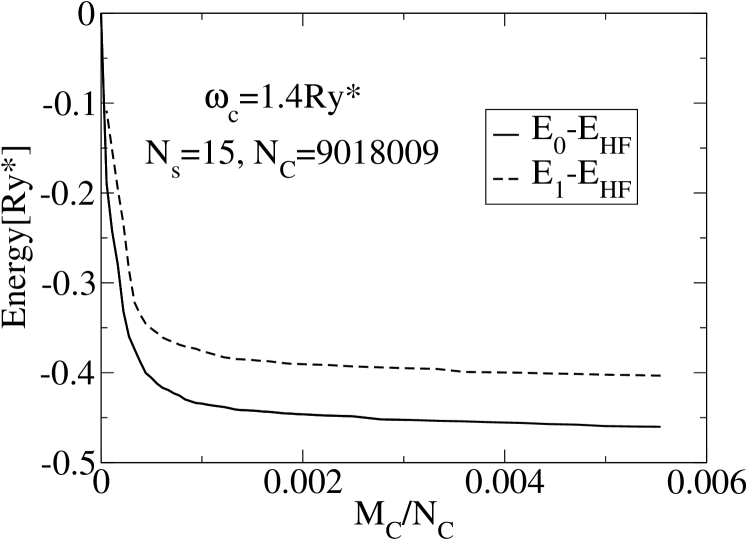
Figure 7: The ground state energy and the first excited state energy in URHF-CI method is shown.

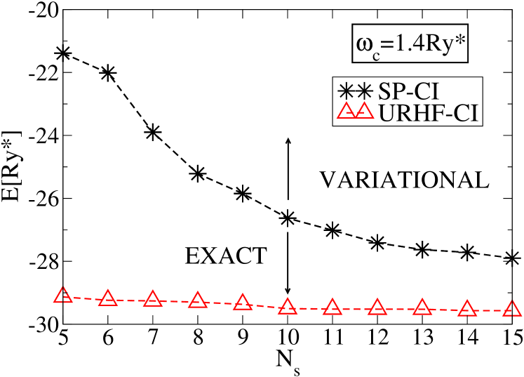
Figure 8: The dependence of URHF-CI and SP-CI ground state energies on $N_{s}$. The pre-calculated direct and exchange energies in URHF-CI improves the ground state energy and the convergence rate. Up to $N_{s}=10$ the SP-CI and URHF-CI Hamiltonian have been diagonalized exactly. Above $N_{s}=10$ the variational ground state energies are calculated by diagonalizing $H_{\rm eff}$ with $M_{C}=63504$.

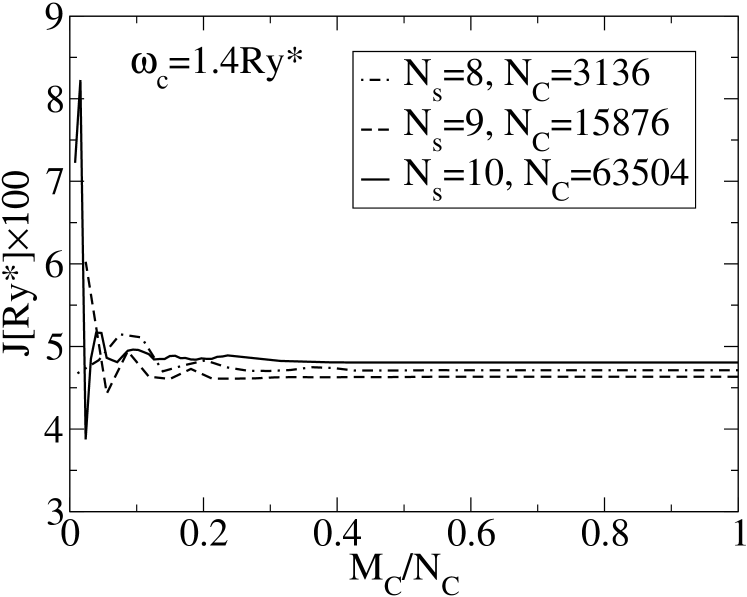
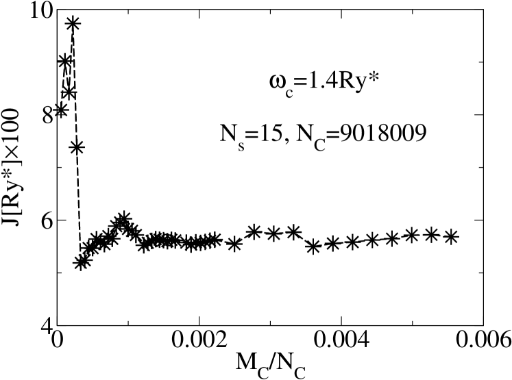
Figure 9: The exchange energy, the spin singlet-triplet energy gap in URHF-CI method is shown. At $\hbar\omega_{c}=1.4Ry^{*}$ the spin singlet state is the ground state.

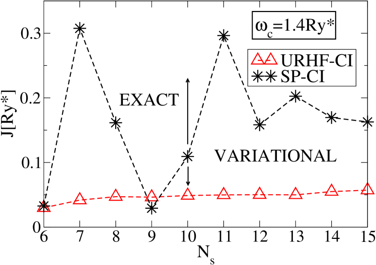
Figure 10: A comparison between the exchange coupling $J$ calculated in SP-CI and URHF-CI is shown. Up to $N_{s}=10$ the SP-CI and URHF-CI Hamiltonian have been diagonalized exactly. Above $N_{s}=10$ a variational calculation has been used by diagonalizing $H_{\rm eff}$ with $M_{C}=63504$.

In the configuration interaction method the Hamiltonian of an interacting system is calculated in the basis of finite number of many-electron configurations. The total number of configurations (or Slater determinants participating in CI calculation) is determined by $N_{C}=[N_{s}!/N_{\uparrow}!(N_{s}-N_{\uparrow})!][N_{s}!/N_{\downarrow}!(N_{s}-N_{\downarrow})!]$. Here $N_{\uparrow}$ and $N_{\downarrow}$ are the number of spin up and spin down electrons. This Hamiltonian is either diagonalized exactly for small systems or low energy eigenvalues and eigenstates are extracted approximately for very large number of configurations. In URHF-CI (SP-CI), $N_{s}$ URHF (single particle) orbitals are used for constructing the Slater determinants. By removing electrons from the occupied URHF state obtained by minimizing the total Hartree-Fock energy and putting them onto an unoccupied URHF state, one can construct a number of configurations corresponding to electron-hole excitations. These excitations contribute to the many body wave functions as correlations.

Denoting the creation (annihilation) operators for URHF quasi-particles by $c^{\dagger}_{i}$ ($c_{i}$) with the index $i$ representing the combined spin-orbit quantum numbers, the many body Hamiltonian of the interacting system in the URHF basis can be written as:

$$H=\sum_{ij}\langle i|T|j\rangle c^{\dagger}_{i}c_{j}+\frac{1}{2}\sum_{ijkl}V_{ijkl}c^{\dagger}_{i}c^{\dagger}_{j}c_{k}c_{l},$$ (8)

where $V_{ijkl}$ are the Coulomb matrix elements in the URHF basis. Our method of computing Coulomb matrix elements is presented in the appendix. Here

$$\langle i|T|j\rangle=\epsilon_{i}\delta_{ij}-\langle i|V_{H}+V_{X}|j\rangle,$$ (9)

where $\epsilon_{i}$ are the URHF eigenenegies, and $V_{H}$ and $V_{X}$ are the Hartree and exchange operators. The Hamiltonian matrix is constructed in the basis of configurations with definite $S_{z}$, and diagonalized using conjugated gradient methods. As the size of URHF basis goes to infinity, the method becomes exact. In practice, one may, however, be able to obtain accurate results using finite number of basis in CI calculation.

To introduce a systematic method for constructing the Hamiltonian, we select a class of configurations which have the highest contribution to the ground state wavefunction. Because the main contribution to the ground state energy of many electron system comes from the Slater determinants formed by the lowest energy HF orbitals, we accept Slater determinants whose HF energies are below an energy cut-off $E_{C}$. The number of such Slater determinants is finite, and is given by $M_{C}$.

The many body Hamiltonian matrix constructed in this way is the following:

$$H = \left(\begin{array}[]{cccccc}H_{11}&H_{12}&&H_{1M_{C}}&&\\ H_{21}&H_{22}&&H_{2M_{C}}&&\\ &&&&&\\ H_{M_{C}1}&H_{M_{C}2}&&H_{M_{C}M_{C}}&&\\ &&&&&\\ &&&&&H_{N_{C}N_{C}}\end{array}\right)$$ (19)

$$=\left(\begin{array}[]{cc}H_{\rm eff}&G\\ G^{\dagger}&Q\end{array}\right)$$

Here $H_{11}<H_{22}<\dots<H_{M_{C}M_{C}}<\dots<H_{N_{C}N_{C}}$ are the HF matrix elements with $H_{11}=E_{HF}$, and $H_{M_{C}M_{C}}=E_{C}$ (the Coulomb interactions in the diagonal elements account for the direct and exchange interactions).

To test this method numerically we set the cyclotron energy to $\hbar\omega_{c}=1.4Ry^{*}$, which corresponds to the crossing and mixing of many orbitals, as shown in Fig. 2. Fig. 5 shows the evolution of URHF electron-hole excitation spectrum as a function of cut-off $M_{C}$. The energy bandwidth $W=H_{N_{C}N_{C}}-E_{HF}$ is finite. As it is illustrated in the inset of Fig. 5, the peak of URHF density of states (DOS) is in the middle of the band. As it is shown in Fig. 6, the diagonal elements of the Hamiltonian $H$ (URHF eigen-energies) can be represented approximately by $E_{C}=E_{HF}+Wf(M_{C}/N_{C})$ where $f(x)$ is a universal function. By increasing $N_{C}$, the total number of URHF eigen-states $M_{C}$ (corresponding to given $E_{C}$) increases. In this case, it is possible to find a lower energy variational wave function if the energy cutoff of $H_{\rm eff}$ is set to a given $E_{C}$.

We now turn to investigate the convergence rate of the calculated ground state energy as a function of cutoff $N_{C}$ and $M_{C}$. In Fig. 7 the energies, measured from the HF energy, of the ground and the first excited state for $N=10$ electrons obtained using URHF basis with $N_{s}=10$ and with $N_{s}=15$ orbitals. We note that for $N=10$ and $N_{s}=10$ the number of configurations $N_{C}=63504$ while for $N_{s}=15$ and $N=10$, $N_{C}=9018009$. Hence for $N_{s}=10$ the Hamiltonian can be diagonalized exactly and the ground and excited states are known up to $M_{C}=N_{C}$. This is not the case for $N_{s}=15$ where we were able to extract the ground and excited states up to $M_{C}=0.006N_{C}$, and exact energies are not known.

However, in both cases the energies fall off rapidly and very quickly saturate as a function of $M_{C}/N_{C}$. Hence it appears sufficient to use only a fraction of low energy configurations to construct the effective Hamiltonian $H_{\rm eff}$ in order to achieve satisfactory convergence.

Given the convergence criteria established above, we now discuss the advantages of URHF-CI versus much easier to use SP-CI, a central result of this work. Fig. 8 shows the dependence of URHF-CI and SP-CI ground state energy on the number of single particle orbitals $N_{s}$ for $N=10$ electron droplet at magnetic field corresponding to $\hbar\omega_{c}=1.4Ry^{*}$. Up to $N_{s}=10$ the SP-CI and URHF-CI Hamiltonian have been diagonalized exactly. Above $N_{s}=10$ the variational ground state energies are calculated by diagonalizing $H_{\rm eff}$ with $M_{C}=63504$. The lowest number of single particle orbitals populated by $N=10$ electrons with $S_{z}=0$ is $N_{s}=5$. For $N_{s}=5$ in SP-CI electrons populate the lowest five single particle orbitals while in URHF electrons populate the HF orbitals, which minimize not only single particle energy but also direct and exchange energy. Hence the starting energy of initial single configuration in URHF-CI has significantly lower energy compared to SP-CI. As the number of available states $N_{s}$, and hence the number of electron-hole excitations (configurations) increases, the ground state energy obtained in URHF-CI decreases very slowly. It starts with Hartree-Fock value of $E=-29.13Ry^{*}$ for $N_{s}=5$ and ends up with $E=-29.6Ry^{*}$ for $N_{s}=15$. This gives our best estimate of total correlation energy of $E_{C}=0.47Ry^{*}$. We find the correlation energy to be only two percent of Coulomb energy.

By contrast with URHF-CI the SP-CI calculations using the single particle basis converge very slowly. The slow convergence can be understood in terms of large direct and exchange energy contribution which the SP-CI attempts to compute very inefficiently. Hence clear advantage in using URHF-CI versus SP-CI method.

We now turn to the analysis of the excitation gaps. We focus on the energy gap between the spin singlet $S=0$ ground state and the spin triplet $S=1$ excited state, the exchange energy $J$.

In Figs. 9 the convergence of calculated exchange energy $J$ as a function of the number of configurations $M_{C}/N_{C}$ is shown for increasing size $N_{s}$ of single particle basis. We see that increasing the size $M_{C}$ of the effective Hamiltonian initially leads to rapid oscillations in $J$ followed by a smooth dependence. These calculations allow us to adjust $M_{c}$ to extract numerically stable exchange energy $J$ for each size of the single particle basis $N_{s}$.

This allows us to compare the dependence of calculated exchange energy using the URHF-CI and SP-CI methods. Fig. 10 shows clearly fluctuations of $J$, calculated using SP-CI method , with increasing number of configurations. These fluctuations can be traced back to many level crossings in single particle orbitals. We are unable to extract reliable value of $J$ using the commonly used SP-CI. By contrast, exchange energy $J$ calculated using URHF-CI shows a smooth and convergent behavior as a function of $N_{s}$.

V.1 HF-CI vs SP-CI - Dependence on the number of electrons N

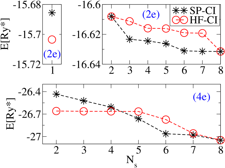
Figure 11: Shown SP-CI and URHF-CI ground state energies vs. number of single particle levels used in CI calculation $(N_{s})$ for two electrons (top) and 4 electrons (bottom) at $\hbar\omega_{c}=1.4Ry^{*}$. For two electrons, although, the ground state energy calculated from URHF is lower than single configuration SP-CI (top-left), but as the number of configurations increases, SP-CI method gives lower energy ground state (top-right). For four electrons, the URHF-CI ground state energy is lower than the one calculated by SP-CI for small number of configurations. As the number of configurations increases, the ground state energy calculated by SP-CI becomes the lowest.

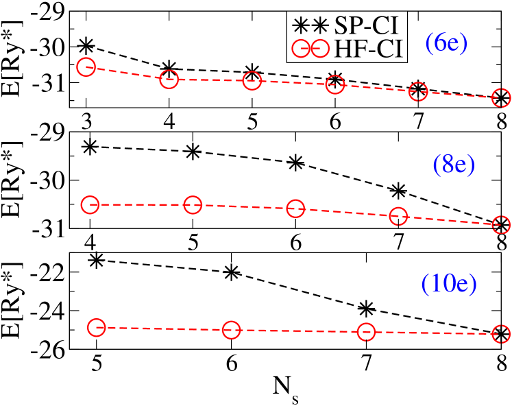
Figure 12: A comparison between SP-CI and URHF-CI ground state energies for six (top), eight (middle) and ten electrons (bottom) at $\hbar\omega_{c}=1.4Ry^{*}$ is shown. In contrast to two and four electron numbers, URHF-CI ground state energy is lower than SP-CI ground state energy for all configurations.

As we discussed in last subsection, computing the spectrum of the CI Hamiltonian requires diagonalization of large matrices. The size of CI Hamiltonian matrices can be optimized significantly by a judicious choice of basis.

In preceding subsection, we introduced URHF states as a suitable basis for CI method. In this subsection, we present a systematic comparison between the ground state energy calculated by URHF-CI and SP-CI methods to remark that URHF-CI is a superior method to deal with a system with large number of electrons. We examine this in quantum dot molecules and in single dot parabolic confining potentials. In quantum dot molecules, we calculate the ground state energy of a system consisting of two to ten electrons. To compare URHF-CI and SP-CI, one must study the behavior of the spectrum as a function of $N_{s}$, and $N_{l}(\geq N_{s})$. With increasing number of configurations, this comparison is carried out up to the point that $N_{s}=N_{l}$, where all possible HF configurations are being exhausted. In the limit of $N_{s}=N_{l}$, there exists a unitary transformation which maps URHF-CI Hamiltonian to SP-CI Hamiltonian, and thus the spectrum of SP-CI and URHF-CI become identical. Because the number of configurations grows rapidly by increasing $N_{s}$, and because we would like to reach the limit of $N_{s}=N_{l}$, we construct URHF states out of small number of single particle levels. For the purpose of this comparison and without any loss of generality we present the results of our calculation using $N_{l}=8$ in Figs. 11-12. In the case of two electrons, URHF energy is lower than the energy of SP-CI with single Slater determinant, $N_{s}=1$, (see the top-left of Fig. 11). By increasing the number of configurations we observe that SP-CI quickly lowers the ground state energy until $N_{s}=8$ where URHF-CI and SP-CI become equivalent. In the case of four electrons, the ground state energy of URHF-CI is lower for small number of configurations. Similar to the two electron system, with increasing number of configurations (beyond $N_{s}=5$) SP-CI provides lower ground state energy. However, with increasing number of electrons from six up to ten, we find that URHF-CI method gives lower ground state energy within the whole range of $N_{s}$, as shown in Fig. 12.

A similar comparison can be made for electrons in a single dot with parabolic confining potential. The energy difference calculated by SP-CI and URHF-CI, presented in Fig. 13, reveals that for electron numbers between two and five, the ground state energy of SP-CI is lower than the ground state energy of URHF-CI. As expected, this order is reversed with increasing number of electrons ($N\geq 6$).

We therefore find URHF-CI method to work very well for quantum dot systems with large number of electrons.

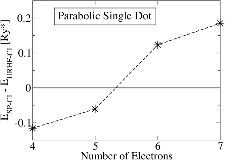
Figure 13: Shown a zero magnetic field comparison between GS energies calculated by SP-CI and URHF-CI methods using $N_{s}=10$, $N_{l}=28$ for a single dot parabolic potential ($\omega_{0}=0.55Ry^{*}$) with electron numbers between $N=4$, and 7. The calculated ground state energy of URHF-CI (SP-CI) is lower for a system with large (small) number of particles.

VI conclusion

We have developed real space unrestricted hybrid Hartree Fock (HF) and configuration interaction (CI) method (URHF-CI) suitable for the calculation of ground and excited states of large number of electrons localized by complex gate potentials in quasi-two-dimensional quantum dot molecules. The effects of magnetic field and correlations are included in energies and directly in the many-particle wavefunctions making the method an attractive candidate for potential quantum information related applications. The advantages of URHF-CI method over the commonly used CI method based on single particle orbitals SP-CI are demonstrated.

VII Acknowledgement

R.A. and P.H. acknowledge the support by the NRC High Performance Computing project and by the Canadian Institute for Advanced Research.

VIII Appendix: Coulomb matrix elements

In this appendix, we describe an efficient approach to calculate Coulomb matrix elements numerically. In the Hartree-Fock and configuration interaction method, the properties of the system are given by the single particle spectrum and by the Coulomb matrix elements defined as two-electron integrals (see Eq. [4]). For the calculation involving 60 HF orbitals the total number of multi-dimensional integrals exceeds $12\times 10^{6}$. Here we describe an efficient algorithm used in our calculation. In the numerical calculation of URHF-CI, the integrals of the Coulomb matrix elements are replaced by summation over the grids $\vec{r}=(ih_{x},jh_{y},kh_{z})$ (where $\{ijk\}$ are integers, and $\{h_{x},h_{y},h_{z}\}$ are grid spacing)

$$V_{\alpha\beta\mu\nu} = \sum_{{\vec{r}}_{1},{\vec{r}}_{2}}\Delta{\vec{r}}_{1}\Delta{\vec{r}}_{2}~{}\psi_{\alpha}^{\ast}({\vec{r}}_{1})\psi_{\nu}({\vec{r}}_{1})$$ (21)

$$\frac{e^{2}}{\epsilon|{\vec{r}}_{1}-{\vec{r}}_{2}|}~{}\psi_{\beta}^{\ast}({\vec{r}}_{2})\psi_{\mu}({\vec{r}}_{2}).$$

We further transform multi-dimensional wave function $\psi_{\alpha}({\vec{r}})$ into a column vector $\psi_{\alpha}(q)$ by mapping the multi-dimensional vector ${\vec{r}}$ onto a one-dimensional index $\{ijk\}\rightarrow q$ where $q=1,2,\dots,N_{x}N_{y}N_{z}$. Then the multi-dimensional integral can be converted into a vector-matrix multiplication

$$V_{\alpha\beta\mu\nu}=\sum_{q,q^{\prime}}\Phi_{\alpha\nu}(q)~{}U(q,q^{\prime})~{}\Phi_{\beta\mu}(q^{\prime})$$ (22)

where $\Phi_{\alpha\nu}(q)=\psi^{*}_{\alpha}(q)\psi_{\nu}(q)$ is a vector containing all the possible pairs of single-particle wave functions, and $U$ is the matrix with elements $\frac{e^{2}}{\epsilon|{\vec{r}}_{1}-{\vec{r}}_{2}|}$ times $\Delta{\vec{r}}_{1}\Delta{\vec{r}}_{2}$. The sums in form of do-loops can be further parallelized. Due to the large dimension of matrix $U$, one can make use of domain decomposition to divide it into a number of smaller matrices and sum up the result of all the individual multiplications.

References

- (1) A. Galindo and M. A. Martin-Delgado, Rev. Mod. Phys. 74, 347 (2002).
- (2) J. A. Brum, and P. Hawrylak, Superlattices Microstruct. 22, 431 (1997).
- (3) D. Loss and D.P. DiVincenzo, Phys. Rev. A 57, 120 (1998); G. Burkard, D. Loss and D. P. DiVincenzo, Phys. Rev. B 59, 2070 (1999).
- (4) A. Szabo and N. S. Ostlund, Modern Quantum Chemistry (McGraw-Hill, New York, 1989).
- (5) L. Jacak, P. Hawrylak, and A. Wojs, Quantum Dots (Springer, Berlin, 1998).
- (6) P.A. Maksym and T. Chakraborty, Phys. Rev. Lett. 65, 108 (1990).
- (7) U. Merkt, J. Huser, and M. Wagner, Phys. Rev. B 43, 7320 (1991).
- (8) D. Pfannkuche, V. Gudmundsson, and P.A. Maksym, Phys. Rev. B 47, 2244 (1993).
- (9) P. Hawrylak and D. Pfannkuche, Phys. Rev. Lett. 70, 485 (1993).
- (10) S.-R. Eric Yang, A.H. MacDonald, and M.D. Johnson, Phys. Rev. Lett. 71, 3194 (1993).
- (11) P. Hawrylak, Phys. Rev. Lett. 71, 3347 (1993).
- (12) J.J. Palacios, L. Martin-Moreno, G. Chiappe, E. Louis, and C. Tejedor, Phys. Rev. B 50, 5760 (1994).
- (13) A. Wojs and P. Hawrylak, Phys. Rev. B 51, 10880 (1995).
- (14) J.H. Oaknin, L. Martin-Moreno, J.J. Palacios, and C. Tejedor, Phys. Rev. Lett. 74, 5120 (1995).
- (15) A. Wojs and P. Hawrylak, Phys. Rev. B 53, 10841 (1996).
- (16) P.A. Maksym, Phys. Rev. B 53, 10871 (1996).
- (17) P. Hawrylak, A. Wojs, and J.A. Brum, Phys. Rev. B 54, 11397 (1996).
- (18) A. Wojs and P. Hawrylak, Phys. Rev. B 55, 13066 (1997).
- (19) A. Wojs and P. Hawrylak, Phys. Rev. B 56, 13227 (1997).
- (20) M. Eto, Jpn. J. Appl. Phys. 36, 3924 (1997).
- (21) M. Eto, J. Phys. Soc. Japan 66, 2244 (1997).
- (22) P.A. Maksym, Physica B 249-251, 233 (1998).
- (23) H. Imamura, H. Aoki, and P.A. Maksym, Phys. Rev. B 57, R4257 (1998).
- (24) H. Imamura, H. Aoki, and P.A. Maksym, Physica B 249-251, 214 (1998).
- (25) P. Hawrylak, C. Gould, A.S. Sachrajda, Y. Feng, and Z. Wasilewski, Phys. Rev. B 59, 2801 (1999).
- (26) C.E. Creffield, W. Häusler, J.H. Jefferson, and S. Sarkar, Phys. Rev. B 59, 10719 (1999).
- (27) N.A. Bruce and P.A. Maksym, Phys. Rev. B 61, 4718 (2000).
- (28) S.M. Reimann, M. Koskinen, and M. Manninen, Phys. Rev. B 62, 8108 (2000).
- (29) S.A. Mikhailov, Phys. Rev. B 65, 115312 (2002).
- (30) J. J. Palacios and P. Hawrylak, Phys. Rev. B 51, 1769 (1995).
- (31) J. Kolehmeinen et al. Eur. Phys. J. B 13,731 (2000).
- (32) Xuedong Hu and S. Das Sarma, Phys. Rev. A 64, 042312 (2001), X. Hu and S. Das Sarma, Phys. Rev. A 61, 062301 (2000).
- (33) A.Wensauer, M.Korkusinski,P.Hawrylak, Phys.Rev.B 67, 035325, (2003).
- (34) A.Wensauer, M.Korkusinski,P.Hawrylak, Solid State Comm. 130, 115 (2004).
- (35) Ramin M. Abolfath, W. Dybalski, and Pawel Hawrylak, Phys. Rev. B 73, 075314 (2006).
- (36) Massimo Rontani, Carlo Cavazzoni, Devis Bellucci, and Guido Goldoni J. Chem. Phys. 124, 124102 (2006).
- (37) D. Yoshioka, B. I. Halperin, and P. A. Lee Phys. Rev. Lett. 50, 1219 (1983).
- (38) F. D. M. Haldane and E. H. Rezayi Phys. Rev. Lett. 54, 237 (1985).
- (39) E. H. Rezayi and F. D. M. Haldane, Phys. Rev. B 32, 6924 (1985); ibid, 33, 7309 (1986).
- (40) G. Fano, F. Ortolani, and E. Colombo Phys. Rev. B 34, 2670 (1986).
- (41) C. Yannouleas and U. Landman, Phys. Rev. Lett. 82, 5325 (1999), Constantine Yannouleas and Uzi Landman, Phys. Rev. B68, 035325 (2003), C. Yannouleas and U. Landman, J. Phys.: Condens. Matter 14, L591 (2002), C. Yannouleas and U. Landman, Int. J. Quantum Chem. 90, 699 (2002).
- (42) B. Reusch, W. Häusler, and H. Grabert, Phys. Rev. B 63, 113313 (2001).
- (43) M. Koskinen, M. Manninen, and S.M. Reimann, Phys. Rev. Lett. 79, 1389 (1997).
- (44) D.G. Austing, S. Sasaki, S. Tarucha, S.M. Reimann, M. Koskinen, and M. Manninen, Phys. Rev. B 60, 11514 (1999).
- (45) K. Hirose and N.S. Wingreen, Phys. Rev. B 59, 4604 (1999).
- (46) O. Steffens and M. Suhrke, Phys. Rev. Lett. 82, 3891 (1999).
- (47) A. Wensauer, O. Steffens, M. Suhrke, and U. Rössler, Phys. Rev. B 62, 2605 (2000).
- (48) A. Wensauer, J. Kainz, M. Suhrke, and U. Rössler, phys. stat. sol. (b) 224, 675 (2001).
- (49) Min Zhuang, Philippe Rocheleau, and Matthias Ernzerhof J. Chem. Phys. 122, 154705 (2005).