Coulomb drag between two spin incoherent Luttinger liquids

Abstract

In a one dimensional electron gas at low enough density, the magnetic (spin) exchange energy $J$ between neighboring electrons is exponentially suppressed relative to the characteristic charge energy, the Fermi energy $E_{F}$. At non-zero temperature $T$, the energy hierarchy $J\ll T\ll E_{F}$ can be reached, and we refer to this as the spin incoherent Lutinger liquid state. We discuss the Coulomb drag between two parallel quantum wires in the spin incoherent regime, as well as the crossover to this state from the low temperature regime by using a model of a fluctuating Wigner solid. As the temperature increases from zero to above $J$ for a fixed electron density, the $2k_{F}$ oscillations in the density-density correlations are lost. As a result, the temperature dependence of the Coulomb drag is dramatically altered and non-monotonic dependence may result. Drag between wires of equal and unequal density are discussed, as well as the effects of weak disorder in the wires. We speculate that weak disorder may play an important role in extracting information about quantum wires in real drag experiments.

I Introduction

In recent years correlated electron systems at the nanoscale and in reduced dimensions have attracted much attention.Manoharan et al. (2000); Nygard et al. (2000); Jarillo-Herrero et al. (2005) In one spatial dimension electron correlations are expected to be enhanced, leading to the so called Luttinger liquid (LL) state.Haldane (1981); Voit (1995) The existence of the LL liquid state in a one dimensional electron system is now an established experimental fact,Ishii et al. (2003); Bockrath et al. (1999); Yao et al. (1999) with direct measurements of the distinct spin and charge velocities in momentum resolved tunneling (as predicted by the theory) providing compelling evidence.Auslaender et al. (2002, 2005)

Another way to explore the correlations in one dimensional systems is in a drag experiment between two parallel quantum wires or nanotubes.Yamamoto et al. (2002); Debray et al. (2001, 2002) (Recall that in most cases the bare conductance of a quantum wire is $2e^{2}/h$ per transverse channel regardless of the electron interactions,Maslov and Stone (1995); Safi and Schulz (1999) and so does not reveal information about electron correlations. An exception to this quantization condition is the situation discussed by Matveev in Refs. Matveev, 2004a, b.) The typical drag set-up involves a current driven in a “active” wire while a voltage drop is measured in a “passive” wire. See Fig. 1.

Figure 1: Coulomb drag schematic. Two quantum wires are arranged parallel to one another. A dc current $I_{1}$ flows in the “active” wire 1 and a voltage bias $V_{2}$ is measured in the “passive” wire 2 when $I_{2}=0$.

The quantity often taken to describe the drag effect is the “drag resistivity” (drag per unit length) defined as

$$r_{D}=-\lim_{I_{1}\to 0}\frac{e^{2}}{h}\frac{1}{L}\frac{dV_{2}}{dI_{1}}\;,$$ (1)

where $V_{2}$ is a voltage induced in wire 2 (the “passive” wire) due to a current $I_{1}$ in wire 1 (the “active” wire). Here $e$ is the charge of the electron, $h$ Planck’s constant, and $L$ the length of the wire. The sign of the drag can be either positive or negative, but it is generally positive (note minus sign in formula) for repulsive interactions between electrons.

Typically, one is interested in the dependence of $r_{D}$ on the temperature, the interwire spacing, the electron density and Fermi wave vector in each wire, the disorder, the wire length, and possibly on an external magnetic field. Physically drag is the result of collisions (momentum transfer) from electrons in the active wire which tend to “push” or “pull” the electrons in the passive wire. Electrons in the passive wire move under these collisions until an electric field is built up in the passive wire (due to a non-uniform density of electrons there) which just cancels the force of the momentum transfer of the electrons in the active wire. This is the physics behind the well known drag formulas of Zheng and MacDonald,Zheng and MacDonald (1993) and Pustilnik et al.Pustilnik et al. (2003) (See Eq. (7).)

While the experimental data on drag between quantum wires is limited,Yamamoto et al. (2002); Debray et al. (2001, 2002) a fair amount of theoretical work has been published. Various studies have made use of LL theory,Fuchs et al. (2005); Klesse and Stern (2000); Nazarov and Averin (1998); Schlottmann (2004a); Flensberg (1998) Fermi liquid (FL) theory withRaichev and Vasilopoulos (2000) and withoutPustilnik et al. (2003) multiple sub-bands, effects of inter-wire tunneling,Raichev and Vasilopoulos (1999) effects of disorder,Ponomarenko and Averin (2000) shot noise correlations,Gurevich and Muradov (2000); Trauzettel et al. (2002) mesoscopic fluctuations,Mortensen et al. (2002, 2001) and the effects of different signs of electron exchange interactions in the wires.Schlottmann (2004b) Additionally, phonon mediated drag has been studied in one dimension.Muradov (2002); Raichev (2001) The main qualitative difference that is found between the LL and FL approaches is whether $r_{D}$ tends to increase (LL) or decrease (FL) as the temperature is reduced to the lowest values. For the case of two infinitely long indentical clean wires the following results are obtained: In a LL, electrons tend to “lock” into a commensurate state at the lowest tempertures giving rise to a diverging drag, while in a FL the phase space available for scattering tends to zero as the temperature is lowered, implying a vanishing drag. For two non-identical wires the drag is usually significantly suppressed at low temperatures relative to the drag in the identical case.Pustilnik et al. (2003); Fuchs et al. (2005)

In spite of the theoretical effort, a number of open questions remain. In particular, the drag effect is known to be strongest when the electron density is low, Yamamoto et al. (2002); Debray et al. (2001, 2002) which typically implies that electron interactions are strong, or equivalently that $r_{s}\equiv a/(2a_{B})$ is large with $a=n^{-1}$ and $a_{B}$ the Bohr radius. For very strong interactions, there is an exponential separation of the spin exchange energy, $J$, and the characteristic charge energy, $E_{F}$, which at finite temperatures can lead to incoherent (thermally excited) spin degrees of freedom while the charge degrees of freedom remain approximately coherent and close to their ground state.Matveev (2004a, b) This energy hierarchy at finite temperature $T$, $J\ll T\ll E_{F}$, we refer to as the spin incoherent Luttinger liquid regime. Already there is mounting understanding of how such spin incoherent Luttinger liquids behave in the Green’s function,Cheianov and Zvonarev (2004a, b); Fiete and Balents (2004) in the momentum distribution function,Cheianov et al. (2005) in momentum resolved tunneling,Fiete et al. (2005a) and in transport.Matveev (2004a, b); Fiete et al. (2005b); Kin

Our goal in this work is to explore some of the implications of spin incoherence on the drag between two quantum wires. We consider only the simplest case of a single channel wire. We attempt to elucidate what qualitative and quantitative changes one can expect for the Coulomb drag when the temperature is much smaller or larger than $J$. Since $J/E_{F}$ is expontially small,Matveev (2004a, b) a small change in the temperature can induce a dramatic change in the temperature dependence of the drag. Based on earlier work of the authors,Fiete et al. (2005b) we are able to discuss the drag deep in the spin incoherent regime in terms of spinless electrons using a simple mapping between the charge variables of the charge sector of a LL with spin and the variables of a spinless LL.

The crossover to the spin incoherent regime is discussed using a model of a fluctuating Wigner solid with an antiferromagnetic Heisenberg spin chain in the spin sector. Distortions of the solid couple the spin and charge degrees of freedom. The model allows us to quantitatively address the crossover. The main result is that as the temperature increases from zero to above $J$ for a fixed electron density, the (already weak) $2k_{F}$ oscillations in the density-density correlations are rapidly lost. As a result, the drag is dramatically suppressed (when $k_{F}d\gtrsim 1$) since forward scattering contributions vanish in the LL model and the Wigner solid model, and $4k_{F}$ contributions are suppressed relative to $2k_{F}$ contributions by $\tilde{U}(4k_{F})/\tilde{U}(2k_{F})\sim e^{-2k_{F}d}\;{\rm for}\;k_{F}d\gtrsim 1$. Here $\tilde{U}(kd)$ is the Fourier transform of the interwire electron-electron interaction, $d$ is the interwire separation, and $k_{F}\equiv\pi/(2a)$ is the Fermi wavevector. See Fig. 2.

Figure 2: Schematic of the possible temperature dependence of the Coulomb drag in a wire of sufficiently low electron density that $J\ll E_{F}\lesssim\omega_{0}$. The non-monotonic temperature dependence shown can be obtained for $K_{c}>1/2$ and $\tilde{U}(4k_{F})\ll\tilde{U}(2k_{F})$ which may be realized for widely space wires. The temperature $T^{*}$ is the “locking” temperature of two identical wires, below which the drag exhibits activated behavior and $E_{s}$ is an energy gap associated with the “locking”. In this paper we consider only temperatures $T>T^{*}$ and investigate the limits $T<J$ and $T>J$, as well as the crossover between the two. When $J\ll E_{F}$ a sharp drop in the drag resistance should be observable for $T\sim J$.

In addition to a possible dramatic suppression (depending on various physical parameters) of the drag, a non-monotonic dependence on temperature may also occur, as illustrated schematically in Fig. 2. Specifically, when $T>T^{*}$, where $T^{*}$ is the “locking” temperature (see Sec. II below), we find that the temperature dependence of the drag is given by

$$r_{D}=C_{1}T^{\alpha_{2k_{F}}}f(T/J)+C_{2}T^{\alpha_{4k_{F}}},$$ (2)

where $f(X\to 0)\to 1$ and $f(X\gtrsim 1)\sim e^{-cX}$, with $c$ a constant of order one. The coefficients $C_{1}\propto\tilde{U}(2kF)$ and $C_{2}\propto\tilde{U}(4kF)$. The exponents $\alpha_{2k_{F}/4k_{F}}$ depend on the interactions in the wires and on the presence or absence of disorder. We find

$$\alpha_{2k_{F}} = 2K_{c}-1\hskip 28.45274pt{\rm clean},$$ (3)

$$= 2K_{c}\hskip 28.45274pt{\rm disordered}\;,$$

and

$$\alpha_{4k_{F}} = 8K_{c}-3\hskip 42.67912pt{\rm clean},$$ (4)

$$= 8K_{c}-2\hskip 28.45274pt{\rm disordered}\;.$$

While it is interesting that disorder changes the temperature dependence of the drag, it may play an even more important role in the measurement of the drag effect itself in actual experiments. The reason is that the drag effect is maximal for identical wires; any $k_{F}$ mismatch results in a drag that is generally strongly diminished relative to this case, indeed, exponentially so at low temperature. Disorder tends to “smear” the momentum structure of the density response that determines the drag, eliminating this exponential suppression. Hence, since in a real experiment one will never have truly identical wires, some residual disorder may actually play a key role in experimental studies of drag between one dimensional systems.

This paper is organized in the following way. In Sec. II we discuss general considerations for drag between two quantum wires with an emphasis on features relevant to the effects of being in the spin incoherent regime. In Sec. III we discuss a model of a fluctuating Wigner solid with a Heisenberg spin chain to describe the magnetic (spin) degrees of freedom. We derive expressions for the density fluctuations of the electron gas by including magneto-elastic coupling that induces $2k_{F}$ density modulations at low temperatures ($T\ll J$) and results in an instability towards a local lattice distortion favoring a spin-Peierls-like state. In Sec. IV we discuss the temperature dependence of the Fourier transform of the density-density correlation function in detail. In Sec. V we discuss the drag itself in detail by considering different temperature regimes, the effects of disorder, and the case of wires with mismatched density. In Sec. VI we summarize the main results of our paper and in the appendicies we give some exact formulas for the density-density correlation function relevant to the spin coherent-incoherent crossover as well as other useful formulas.

II General Considerations

We assume the Hamiltonian of our system is of the form

$$H=H_{1}+H_{2}+H_{12}\;,$$ (5)

where $H_{i}$ is the Hamiltonian in the $i^{th}$ wire and $H_{12}$ describes the interactions between electrons in different wires. A proper drag situation is one in which the tunneling between wires can be neglected. We thus assume that $H_{12}$ allows only interactions which forbid electrons to tunnel between the wires.tun The Hamiltonian $H_{i}$ in principle describes arbitrary interactions between electrons within the $i^{th}$ wire; depending on the particular situation of interest, a number of different models have been proposed from Fermi liquidDebray et al. (2002); Raichev and Vasilopoulos (2000); Pustilnik et al. (2003) to Luttinger liquid.Fuchs et al. (2005); Klesse and Stern (2000); Nazarov and Averin (1998); Schlottmann (2004a); Flensberg (1998)

The Hamiltonian $H_{12}$ is a function of the interwire electron interaction which is often taken to be of the form

$$U_{12}(x)=\frac{e^{2}}{\epsilon}\frac{1}{\sqrt{d^{2}+x^{2}}}\;,$$ (6)

where $e$ is the charge of the electron, $\epsilon$ the dielectric constant of the material, and $d$ the separation between the two wires. The Fourier transform, $\tilde{U}(k)=2(e^{2}/\epsilon)K_{0}(kd)$, depends on the dimensionless parameter $kd$ and for $kd\gg 1,\;\tilde{U}(k)\sim\frac{1}{\sqrt{k}}e^{-kd}$. This exponential dependence of the interwire interaction leads to an exponential dependence of the drag resistivity on wire separation (for large enough $d$) when the drag is dominated by large momentum transfer as it is in the LL model and the model we will discuss in this paper. The following drag formula (or its equivalent) has been derived by Zheng and MacDonaldZheng and MacDonald (1993) for a disordered FL,2Dd by Klesse and SternKlesse and Stern (2000) for a LL, and by Pustilnik et al.Pustilnik et al. (2003) for a clean FL:

$$r_{D}=\int_{0}^{\infty}dk\int_{0}^{\infty}d\omega\frac{k^{2}\tilde{U}^{2}_{12}(k)}{4\pi^{2}n_{1}n_{2}T}\frac{{\rm Im}\chi^{R}_{1}(k,\omega){\rm Im}\chi^{R}_{2}(k,\omega)}{\sinh^{2}(\omega/2T)}\;,$$ (7)

where ${\rm Im}\chi^{R}_{i}(k,\omega)$ is the imaginary part of the Fourier transformed retarded density-density correlation function, Eqs. (IV) and (IV), and $n_{i}$ is the density of the electrons in the $i^{th}$ wire. Knowing the general features of the interwire interaction $U_{12}$, (see Fig. 3) it is clear that to determine the drag one must determine the ${\rm Im}\chi^{R}_{i}(k,\omega)$.

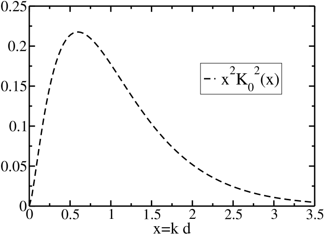
Figure 3: Momentum dependence of the the quantity $k^{2}\tilde{U}^{2}_{12}(k)=\left(\frac{2e^{2}}{\epsilon d}\right)^{2}(xK_{0}(x))^{2}$ appearing in the drag formula Eq. (7) as a function of the dimensionless variable $x=kd$ where we have assumed the real space inter-wire electron interaction (6). Plotted is the quantity $(xK_{0}(x))^{2}$ which has a maximum for $x\approx 0.6.$ For $x\ll 1$, $(xK_{0}(x))^{2}\sim(-\gamma+\ln(2)-\ln(x))^{2}x^{2}$ where $\gamma\approx 0.5772$ is Euler’s constant, while for $x\gg 1$, $(xK_{0}(x))^{2}\sim e^{-2x}.$

We will discuss the behavior of ${\rm Im}\chi^{R}_{i}(k,\omega)$ and its temperature dependence in detail in Sec. IV, but for now it is sufficient to point out that most of weight occurs near momenta of $k\approx 0,\;k\approx 2k_{F}$, and $k\approx 4k_{F}$ so that one may write

$${\rm Im}\chi^{R}_{i}(k,\omega)\approx{\rm Im}\chi_{i}^{R,0}(k,\omega)+{\rm Im}\chi_{i}^{R,2k_{F}}(k,\omega)$$

$$+{\rm Im}\chi_{i}^{R,4k_{F}}(k,\omega).$$ (8)

As we will see, the $2k_{F}$ components of ${\rm Im}\chi^{R}_{i}(k,\omega)$ present at low temperatures, $T\ll J$, will disappear when $T\gg J$. Moreover, once it is known that ${\rm Im}\chi_{i}^{R,0}(k,\omega)\propto\delta(\omega-v_{c,i}k)$ (see Sec. IV) where $v_{c,i}$ is the charge velocity of the $i^{th}$ wire, it is readily seen from Eq. (7) that for the LL model (or any model possessing a harmonic bosonized theory) the $k=0$ contribution to the drag resistivity vanishes (in the absence of disorder), leaving only contributions from the higher $k=2k_{F},4k_{F}$ values of ${\rm Im}\chi^{R}_{i}(k,\omega)$. The higher $k=2k_{F},4k_{F}$ values can be strongly suppressed by the interwire interaction because $\tilde{U}^{2}_{12}(k)\sim e^{-2kd}$ when $kd\gg 1$. Hence, in the limit $k_{F}d\gtrsim 1$ we expect a dramatic reduction in the drag and a change in the temperature dependence of the drag (see below) when $2k_{F}$ oscillations are lost and only $4k_{F}$ modulations remain. However, before we address these details, it is useful to go over what we can say about drag deep in the spin incoherent regime itself.

Based on the results of earlier work,Fuchs et al. (2005); Klesse and Stern (2000) we can immediatly discuss the drag deep within the spin incoherent LL regime, $J\ll T\ll E_{F}$. It has earlier been arguedFiete et al. (2005b) that the spin incoherent LL behaves essentially as a spinless LL by noting that the Hamiltonian is diagonal in spin to lowest order in $J/T\ll 1$, and by demanding the equivalence of the physical charge density in both cases. The equivalence can be summarized by the simple equation $K=2K_{c}$ (in the notation of Klesse and SternKlesse and Stern (2000)) relating the interaction parameter of the spinless LL theory and the interaction parameter of the charge sector of the LL theory with spin. (Strictly speaking, for drag the relevant interaction parameter is $K=K_{-}$, the interaction parameter in the odd channel of the relative density of the two wires,Fuchs et al. (2005); Klesse and Stern (2000) but when the inter-wire interactions are sufficiently weak $K_{-}$ is essentially equal to the correponding parameter of the isolated wire.) The relation $K=2K_{c}$ is valid for any particle conserving operator;Fiete et al. (2005b) the drag resistivity is derived from such an operator. Hence, those general results apply here.

As discussed in Refs. Fuchs et al., 2005; Klesse and Stern, 2000, drag in the spinless LL model comes from the backscattering of electrons. As long as the inter-wire interactions are sufficiently small the effects of backscattering can be treated perturbatively. Based on such a perturbative treatment, Klesse and Stern foundKlesse and Stern (2000) that for identical wires there is a temperature scale $T^{*}$ that separates high and low temperature drag regimes. (It is assumed througout this paper that $T^{*}$ is greater than the thermal length $T_{L}$ so that the Fermi liquid leads attached to the quantum wire are not felt.) For temperatures $T\gg T^{*},T_{L}$, the drag varies as a power of the temperature, while for temperatures $T^{*}\gg T\gg T_{L}$, the drag resistivity shows activated behavior with a gap of order $T^{*}$ itself. The physics is similar to that of a pinned charge density wave. This result follows from an analysis of a sine-Gordon model in the odd channel of the coupled wire problem. Applying the equivalence rule $K=2K_{c}$ discussed above in the spin incoherent regime, we have

$$\rho_{D}\sim T^{8K_{c}-3},\;\;T\gg T^{*},T_{L},J,$$ (9)

$$\rho_{D}\sim e^{E_{s}/T},\;\;T^{*}\gg T\gg T_{L},J,$$ (10)

where $E_{s}\sim T^{*}$.Klesse and Stern (2000) Note that for $3/8<K_{c}<3/4$ the temperature dependence of the spinless (fully polarized) electron gas and the spin incoherent electron gas exhibit very different drag resistivity behavior with temperature when $T>>T^{*}$. (The spinless case has a diverging drag resistivity as $T$ is lowered, while the spin incoherent case has a suppressed drag resistivity as $T$ is lowered.) This is qualitatively similar to the transport results found in Ref. Fiete et al., 2005b for $1/2<g_{c}<1$.

The results (9) and (10) above were derived from a perturbative analysis of the sine-Gordon equation which results from treating the backscattering in LL theory. For most realistic parameter values, the baskcattering strength flows to strong coupling and the resulting state is that of the two quantum wires locked into a “zig-zag” charge pattern. The value of $T^{*}$ depends on details of the quantum wire system such as the density, wire widths, and separation $d$,Klesse and Stern (2000) but for most realistic situations $T^{*}/E_{F}\ll 0.01$.

It is interesting to consider how spin incoherence affects the “zig-zag” locking pattern of the electrons in the two wires. The relative size of $J$ and $T^{*}$ will determine what the periodicity of the “zig-zag” pattern will be for $T<<T^{*}$. For $J\ll T\ll T^{*}$, there is a “$4k_{F}$” locking (seen easily from the $K=2K_{c}$ mappingFiete et al. (2005b)) since $T\gg J$ ensures $2k_{F}$ pieces of the density are washed out, while for $T\ll J,T^{*}$, there is a “$2k_{F}$” locking. Of course, for $T^{*}\ll J\ll T$ the locking phase is not obtained. Throughout this paper we will assume $T\gg T^{*}$ so that we need not be concerned with “locking” from here forward.

Similar arguments to those given in Ref. Fuchs et al., 2005 can also be used to describe the incommensurate-commensurate transition deep in the spin incoherent regime for wires of different electron densities. We now leave generalities behind and turn to a detailed calculation of the drag itself in the regime of very strongly interacting one dimensional electrons.

III The fluctuating Wigner Solid Model

We assume from the outset that the interactions between the electrons are very strong, which typically means the density is low enough that we can treat the electrons in each wire as a harmonic chainNov in the charge sector and a nearest neighbor Heisenberg antiferromagnet in the spin sector:Matveev (2004b); Fiete et al. (2005a)

$$H_{\rm wire}=H_{c}+H_{s}\;,$$ (11)

where

$$H_{c}=\sum_{l=1}^{N}\frac{p_{l}^{2}}{2m}+\frac{m\omega_{0}^{2}}{2}(u_{l+1}-u_{l})^{2}\;,$$ (12)

is the Hamiltonian in the charge sector with $p_{l}$ the momentum of the $l^{th}$ electron, $u_{l}$ the displacement from equilibrium of the $l^{th}$ electron, $m$ the electron mass, and $\omega_{0}$ the frequency of local electron displacements (this will depend on the electron density, the width of the wires, the dielectric constant of the material, and other parameters such as the distance to a nearby gateGlazman et al. (1992); Häusler et al. (2002)). The position of the electrons along the chain are given by

$$x_{l}=la+u_{l}\;,$$ (13)

where $a$ is the mean spacing of the electrons. The Hamiltonian of the spin sector takes the form

$$H_{s}=\sum_{l}J_{l}{\vec{S}_{l+1}}\cdot{\vec{S}_{l}}\;.$$ (14)

Note that in (14) the coupling $J_{l}$ between spins depends on the distance between them. Assuming that the fluctuations from the equilibrium positions are small compared to the mean particle spacing, we can expand the exchange energy as

$$J_{l}=J_{0}+J_{1}(u_{l+1}-u_{l})+{\cal O}((u_{l+1}-u_{l})^{2})\;.$$ (15)

In this case the full Hamiltonian takes the form

$$H=H_{c}+H_{s}+H_{s-c}\;,$$ (16)

where

$$H_{s-c}=J_{1}\sum_{l}(u_{l+1}-u_{l}){\vec{S}_{l+1}}\cdot{\vec{S}_{l}}\;.$$ (17)

Here $H_{s-c}$ represents a magneto-elastic coupling as it couples the magnetic modes to the elastic distortions of the lattice that constitute the charge modes.

Our goal is to evaluate the Fourier transform of the retarded density-density correlation function $-i\theta(t-t^{\prime})\langle[\rho(x,t),\rho(x^{\prime},t^{\prime})]\rangle$ [which appears in the drag formula (7)] up to second order in $J_{1}$ for $T,J_{0}\ll\hbar\omega_{0}$, for both $T\ll J_{0}$ and $T\gg J_{0}$. We use the following definition of the electron density: $\rho(x,t)=\sum_{l}\delta(x-al-u_{l}(t))$. An exact calculation within this model is presented in Appendix A. Here we will pursue an approximate calculation that captures all of the essential features of the more exact perturbative results.

III.1 Low energy approach to charge fluctuations

In this work we are concerned only with energies (temperatures) small compared to the characteristic lattice energy, i.e. $T\ll\hbar\omega_{0}$, but still large compared to the “locking” temperature $T^{*}$. When $T\ll J_{0}$ further approximations that can be made, but for now our only restriction will be that $T\ll\hbar\omega_{0}$. We begin by expanding the displacement of the electron density in a Fourier series. For low energy distortions the $k\approx 0$ component is most important, while the magneto-elastic term (17) couples the $k\approx\pi/a$ component to the spin operator ${\vec{S}_{l+1}}\cdot{\vec{S}_{l}}$. Thus, the displacement, $u_{l}$ of the $l^{th}$ electron in the harmonic chain (12) is approximately given by

$$u_{l}=u_{0}(la)+u_{\pi}(la)(-1)^{l},$$ (18)

where $u_{0}$ refers the $k\approx 0$ component of the displacement and $u_{\pi}$ refers to the $k\approx\pi/a$ displacement. Both $u_{0}$ and $u_{\pi}$ are assumed to be slowly varying functions of position, and we expect $u_{\pi}\ll u_{0}$.

III.1.1 Low energy form of the action

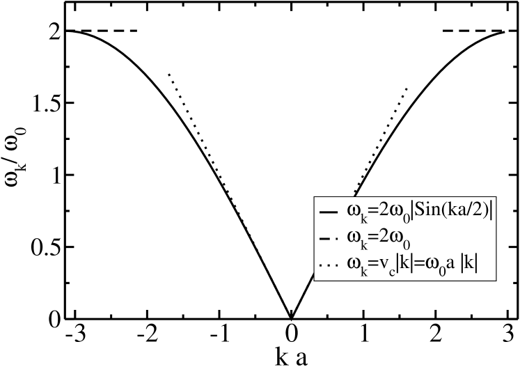
Figure 4: Approximate form for the phonon spectrum. There are two relevant parts of the spectrum that enter the action $S_{c}$, the part near $k\approx 0$ and the part near $k\approx\pi/a$. The phonons with $k\approx 0$ are described by a Debye model while those phonons with $k\approx\pi/a$ are described by an Einstein model.

The action for the low density electron gas is

$$S=S_{c}+S_{s}+S_{s-c}\,.$$ (19)

Using the expression (18) for the particle displacement fields, and noting that from the phonon dispersion of (12), $\omega_{k}=2\omega_{0}|\sin(ka/2)|$, one has for $k\approx 0$ the dispersion $\omega_{k}=v_{c}|k|$ with $v_{c}=\omega_{0}a$, while for $k\approx\pi/a$ the dispersion $\omega_{k}=2\omega_{0}$ is independent of $k$. (See Fig. 4.) In the charge sector we then have the following action of the form $S_{c}=S_{c}^{0}+S_{c}^{\pi}$,

$$S_{c}=\int\frac{dxd\tau}{2\pi}\Biggl{[}\frac{1}{K_{c}v_{c}}\left((\partial_{\tau}\theta_{c}(x,\tau))^{2}+v_{c}^{2}(\partial_{x}\theta_{c}(x,\tau))^{2}\right)$$

$$+m\pi\left((\partial_{\tau}u_{\pi}(x,\tau))^{2}+(2\omega_{0})^{2}u_{\pi}(x,\tau)^{2}\right)\Biggr{]}\;,\hskip 14.22636pt$$ (20)

where $K_{c}=\pi\hbar/(2amv_{c})$. Note the lack of spatial derivative in the $u_{\pi}$ piece of the action which results in the absence of any $k$ dependence in $\omega_{k}$ near $k\approx\pi/a$. In effect, we have described the small $k$ oscillations (phonons) with a Debye-type model and the large $k$ oscillations as an Einstein model. Fig. 4 illustrates the approximations to the full phonon spectrum.

In the standard LL model for weakly interacting electrons $K_{c}=v_{F}/v_{c}\lesssim 1$ where $v_{F}$ is the Fermi velocity of non-interacting electrons. In the present case of strongly interacting electrons we have $K_{c}=\frac{\hbar^{2}\pi}{2ma^{2}}\frac{1}{\hbar\omega_{0}}\sim\frac{E_{F}}{\hbar\omega_{0}}\sim\frac{\rm{Kin}}{{\rm Pot}}\sim\frac{1}{r_{s}}$ where $E_{F}$ is the Fermi energy of non-interacting electrons and $r_{s}\equiv a/(2a_{B})$ where $a_{B}=\epsilon\hbar^{2}/me^{2}$ is the Bohr radius of a material of dielectric constant $\epsilon$. Thus, in the strongly interacting limit $K_{c}$ scales roughly as the ratio of the kinetic energy to the potential energy which itself roughly scales as $r_{s}^{-1}$ implying that very strong (long-range) interactions can lead to small $K_{c}$. In practice, however, $K_{c}$ rarely appears to be smaller than $0.2$ or so.

By making the identification ${\cal E}_{l}\equiv(-1)^{l}{\vec{S}_{l+1}}\cdot{\vec{S}_{l}}\to{\cal E}(x,\tau)$ in the continuum limit, we have spin-charge coupling in the action

$$S_{s-c}=\int\frac{dxd\tau}{2\pi}2J_{1}u_{\pi}(x,\tau){\cal E}(x,\tau)\;.$$ (21)

In the special situation where $T\ll J_{0}$, the action for the spin sector (14) can be bosonized asSachdev (1999); Giamarchi (2004)

$$S_{s}=\int\frac{dxd\tau}{2\pi}\Biggl{[}\frac{1}{K_{s}v_{s}}\left((\partial_{\tau}\theta_{s}(x,\tau))^{2}+v_{s}^{2}(\partial_{x}\theta_{s}(x,\tau))^{2}\right)\Biggr{]}\;,$$ (22)

where the $SU(2)$ symmetry of the Heisenberg model implies that $K_{s}=1$ and the spin velocity is $v_{s}\sim J_{0}a/\hbar$. (Here intrawire backscattering effects in the spin sector have been neglected and a sine-Gordon term dropped. Since we are ultimately interested in energies/temperatures much larger than $J_{0}$ or much smaller than $J_{0}$ this will not affect any of our conclusions.) However, when $T\gtrsim J_{0}$ the action for the spin sector must describe more accurately the short distance physics of the Heisenberg chain. Nevertheless, the action (22) will prove useful in understanding the approach to the spin incoherent regime in the limit $T\to J_{0}$ from below.

Finally, for $T\ll J_{0}$ the coupling term in the action can be expressed asGiamarchi (2004)

$$S_{s-c}=\int\frac{dxd\tau}{2\pi}\frac{2J_{1}}{2\pi\alpha a}u_{\pi}(x,\tau)\sin(\sqrt{2}\theta_{s}(x,\tau))\;,$$ (23)

where we have used the low-energy bosonized form $(-1)^{l}{\vec{S}_{l+1}}\cdot{\vec{S}_{l}}\approx\frac{1}{2\pi\alpha}\sin(\sqrt{2}\theta_{s}(x))$. Here $\alpha={\cal O}(a)$ is a short distance cut off of order the lattice spacing. At low energies this term will lead to the spin-Peierls state indicated in Fig. 5.

III.1.2 Expressing the density

Expanding the density and making use of (18) then gives (we have suppressed the time dependence of $u_{0}$ and $u_{\pi}$ immediately below for clarity of presentation)

$$\rho(x) = \sum_{l}\delta(x-la-u_{l}),$$ (24)

$$= \sum_{l}\delta(x-la-u_{0}(la)+u_{\pi}(la)(-1)^{l}),$$

$$\approx \sum_{l}[\delta(x-la-u_{0}(la))$$

$$\;\;\;\;-\delta^{\prime}(x-la-u_{0}(la))u_{\pi}(la)(-1)^{l})].$$

Multiplying by $\delta(x^{\prime}-la)$, integrating over $x^{\prime}$, and using the Poisson summation identity,

$$\sum_{l}\delta(x^{\prime}-la)=\frac{1}{a}\sum_{m=-\infty}^{\infty}e^{i\frac{2\pi}{a}mx^{\prime}},$$ (25)

the expression for the density becomes

$$\rho(x)\approx\int dx^{\prime}\frac{1}{a}\delta(x-x^{\prime}+u_{0}(x^{\prime}))\sum_{m=-\infty}^{\infty}e^{i\frac{2\pi}{a}mx^{\prime}}$$

$$\times\Bigl{[}1+\cos(\frac{\pi}{a}x^{\prime})\partial_{x^{\prime}}u_{\pi}(x^{\prime})$$

$$+i\frac{\pi}{2a}\left((2m+1)e^{i\frac{\pi}{a}x^{\prime}}+(2m-1)e^{-i\frac{\pi}{a}x^{\prime}}\right)u_{\pi}(x^{\prime})\Bigr{]},$$ (26)

where we have integrated by parts in the second term of (24). Performing the integration over $x^{\prime}$, making use of the approximate relation $\delta(x-x^{\prime}-u_{0}(x^{\prime}))\approx\delta(x^{\prime}-x-u_{0}(x))/|1+\partial_{x}u_{0}(x)|$, and assuming $a\partial_{x}u_{\pi}(x)\ll u_{\pi}(x)$, we find the most important terms up to $4k_{F}$ are

$$\rho(x)\approx\frac{1}{a}(1-\partial_{x}u_{0}(x))\Bigl{[}1-\frac{2\pi}{a}\sin\left(2k_{F}(x+u_{0}(x))\right)u_{\pi}(x)$$

$$+\cos\left(4k_{F}(x+u_{0}(x))\right)\Bigr{]},$$

$$\approx\rho_{0}-\frac{\sqrt{2}}{\pi}\partial_{x}\theta_{c}(x)-\rho_{0}\frac{2\pi}{a}\sin\left(2k_{F}x+\sqrt{2}\theta_{c}(x)\right)u_{\pi}(x)$$

$$+\rho_{0}\cos\left(4k_{F}x+\sqrt{8}\theta_{c}(x)\right),\hskip 14.22636pt$$ (27)

where $\rho_{0}\equiv 1/a$, $k_{F}\equiv\pi/(2a)$, and we have made the identification $u_{0}(x)/a=\sqrt{2}\theta_{c}(x)/\pi$. Recall the field $\theta_{c}$ is governed by the action (III.1.1). This formula resembles the standard bosonized expression for the density of a Luttinger liquid (except for the term $u_{\pi}$ multiplying the $2k_{F}$ part of the density instead of a term involving the spin fields). As we will now see, a formula very similar to that obtained from the standard Luttinger liquid treatment results from integrating out the high energy $u_{\pi}$ phonon modes in favor of the low energy spin modes. To see this, consider only the $2k_{F}$ part of the density and compute $\langle\rho_{2k_{F}}(x,\tau)\rangle$ to lowest order in the action $S_{s-c}$ and integrate out the $u_{\pi}$ fields to obtain a new $\rho_{2k_{F}}^{\rm eff}(x,\tau)$ independent of $u_{\pi}$. At lowest order we find

$$\langle u_{\pi}(x,\tau)\rangle=-\frac{2J_{1}}{\hbar}\int\frac{dx^{\prime}d\tau^{\prime}}{2\pi}{\cal E}(x^{\prime},\tau^{\prime})$$

$$\times\langle T_{\tau}u_{\pi}(x,\tau)u_{\pi}(x^{\prime},\tau^{\prime})\rangle_{S_{c}^{\pi}}\;,$$ (28)

where $T_{\tau}$ is the $\tau$-ordering operator and the $\tau$-ordered product is evaluated in the action $S_{c}^{\pi}$ given in (III.1.1). The $\tau$-ordered product is readily evaluated as

$$\langle u_{\pi}(x,\tau)u_{\pi}(x^{\prime},\tau^{\prime})\rangle_{S_{c}^{\pi}}=\frac{\hbar\delta(x-x^{\prime})}{4m\omega_{0}}$$

$$\times\left[\frac{e^{2\omega_{0}|\tau-\tau^{\prime}|}}{e^{\beta 2\omega_{0}}-1}-\frac{e^{-2\omega_{0}|\tau-\tau^{\prime}|}}{e^{-\beta 2\omega_{0}}-1}\right]\;,$$

$$\to\frac{\hbar\delta(x-x^{\prime})}{4m\omega_{0}}e^{-2\omega_{0}|\tau-\tau^{\prime}|}\;{\rm as}\;\beta\omega_{0}\to\infty.$$ (29)

Recall that we are interested only in temperatures low compared to the phonon energy $\omega_{0}$ so the limit $\beta\omega_{0}\to\infty$ is the appropriate one. Here $\beta=(k_{B}T)^{-1}$ where $k_{B}$ is Boltzmann’s constant. The integral over position in (III.1.2) is immediately evaluated with the delta function in (III.1.2) and the remaining integral over $\tau^{\prime}$ can be approximately evaluated under the assumption $\beta\omega_{0}\to\infty$ which produces the dominant contribution at $\tau^{\prime}\approx\tau$ with a width in $\tau^{\prime}$ of order $1/(2\omega_{0})$ resulting in

$$\langle u_{\pi}(x,\tau)\rangle\approx-\frac{2J_{1}}{16\pi^{2}m\omega_{0}^{2}}{\cal E}(x,\tau)\;,$$ (30)

which yields

$$\rho_{2k_{F}}^{\rm eff}(x,\tau)=\frac{1}{8\pi}\left(\frac{J_{1}}{m\omega_{0}^{2}a^{2}}\right)\sin\left(2k_{F}x+\sqrt{2}\theta_{c}(x,\tau)\right)$$

$$\times{\cal E}(x,\tau).\;\;\;\$$ (31)

The result (III.1.2) is general, and valid whenever $T\ll\hbar\omega_{0}$. However, when $T\ll J_{0}$ one may use the expression ${\cal E}(x,\tau)=\frac{1}{2\pi\alpha}\sin(\sqrt{2}\theta_{s}(x,\tau))$ which leads to the familiar looking density

$$\rho^{\rm eff}(x,\tau)=\rho_{0}-\frac{\sqrt{2}}{\pi}\partial_{x}\theta_{c}(x,\tau)\hskip 99.58464pt$$

$$-\frac{\rho_{0}}{16\pi}\left(\frac{J_{1}}{m\omega_{0}^{2}a^{2}}\right)\sin\left(2k_{F}x+\sqrt{2}\theta_{c}(x,\tau)\right)\sin(\sqrt{2}\theta_{s}(x,\tau))$$

$$+\rho_{0}\cos\left(4k_{F}x+\sqrt{8}\theta_{c}(x,\tau)\right).\hskip 14.22636pt$$ (32)

The expression for the effective density (III.1.2) with the high energy $u_{\pi}$ modes integrated out in favor of the spin variables is valid for $T\ll J_{0}$ and may be compared directly with the LL result obtained for weakly interacting electrons.Voit (1995) At temperatures $T\gg J_{0}$ (III.1.2) must be used for the $2k_{F}$ density variations. The only material difference between (III.1.2) and the standard LL result is the dimensionless ratio of spin and charge energies $\left(\frac{J_{1}}{m\omega_{0}^{2}a^{2}}\right)\sim\frac{v_{s}}{v_{c}}$ which is absent (since it is of order 1) in the familiar LL case. When the interactions are strong as we have assumed them to be here, then $\left(\frac{J_{1}}{m\omega_{0}^{2}a^{2}}\right)\sim\frac{v_{s}}{v_{c}}\ll 1$, since $J_{1}$ diminishes and $\omega_{0}$ increases with increasing strength of the interactions. However, starting from the strongly interacting limit and decreasing the interaction strength the ratio $\left(\frac{J_{1}}{m\omega_{0}^{2}a^{2}}\right)\to 1$. It is worth emphasizing, then, that when the temperature is low compared to both spin and charge energies a 1-d electron gas always behaves as a LL in the sense of the various power laws that will appear in the correlation functions, although the overall prefactors of the $2k_{F}$ pieces will be down by the ratio $\left(\frac{J_{1}}{m\omega_{0}^{2}a^{2}}\right)$. If, on the other hand, the system is in the spin incoherent regime $J_{0}\ll T\ll\hbar\omega_{0}$, the $2k_{F}$ parts of the correlations will be washed out from thermal effects. We now turn to an investigation of how this happens in detail for the case of the density-density correlation function and then discuss the implications for the Coulomb drag between two quantum wires.

IV Evaluation of ${\rm Im}\chi^{R}_{i}(k,\omega)$

Here we consider two limits of the double wire system shown in Fig. 1: (i) Clean wires without disorder and (ii) Wires with weak disorder. The case of strong disorder is uninteresting as the electrons are all localized over the relevant energy/length scales of the experiment. As we discussed in Sec. II, the drag formula (7) generically contains contributions at $k\approx 0,\;k\approx 2k_{F}$, and $k\approx 4k_{F}$ so that ${\rm Im}\chi^{R}_{i}(k,\omega)\approx{\rm Im}\chi_{i}^{R,0}(k,\omega)+{\rm Im}\chi_{i}^{R,2k_{F}}(k,\omega)+{\rm Im}\chi_{i}^{R,4k_{F}}(k,\omega)$. We now turn to an evaluation of each of these pieces. We have used the two standard (equivalent) definitions

$$\chi^{R}_{i}(k,\omega)=-i\int_{-\infty}^{\infty}\!\!\!dx\int_{0}^{\infty}\!\!\!dte^{i((\omega+i\eta)t-kx)}$$

$$\times\langle[(\rho_{i}(x,t)-\rho_{i,0}),(\rho_{i}(0,0)-\rho_{i,0})]\rangle,$$ (33)

and

$$\chi_{i}(k,\omega_{n})=-\int_{-\infty}^{\infty}\!\!\!dx\int_{0}^{\beta}\!\!\!d\tau e^{i(\omega_{n}\tau-kx)}$$

$$\times\langle(\rho_{i}(x,\tau)-\rho_{i,0})(\rho_{i}(0,0)-\rho_{i,0})\rangle,$$ (34)

where $\rho_{i,0}$ is the average density of the $i^{\rm th}$ wire, and $\eta$ is a small infinitesimal that ensures convergence of the time integral in (IV). The retarded correlation function is obtained from (IV) via the substitution $i\omega_{n}\to\omega+i\eta$. We will use both of the formulas above in the subsections that follow.

IV.1 Clean Wires

We first consider wires with no disorder. We will also assume initially that $T\ll J_{0}$ so that we may use the form of the density (III.1.2). (This is only an issue for the evaluation of ${\rm Im}\chi_{i}^{R,2k_{F}}(k,\omega)$ since ${\rm Im}\chi_{i}^{R,0}(k,\omega)$ and ${\rm Im}\chi_{i}^{R,4k_{F}}(k,\omega)$ do not involve the spin sector of the Hamiltonian.) As the authors discussed in Ref. Fiete et al., 2005b the approach to the spin incoherent regime from temperatures well below the spin energy can be understood in this way. In all calculations below, recall that we have assumed the temperature is low, $T\ll\hbar\omega_{0}$, so that the charge sector is always in the LL regime and described by the action $S_{c}^{0}$ in (III.1.1).

IV.1.1 ${\rm Im}\chi_{i}^{R,0}(k,\omega)$

We first evaluate the $k\approx 0$ piece of the retarded density-density correlation function. From the expression (III.1.2), we have

$$\rho^{\rm eff}_{0}(x,t)=\rho_{0}-\frac{\sqrt{2}}{\pi}\partial_{x}\theta_{c}(x,t),$$ (35)

whose correlation function is readily computed (see Appendix B) to yield

$${\rm Im}\chi^{R,0}_{i}(k,\omega)=\frac{k^{2}}{a^{2}}\frac{\hbar L}{2m\omega_{k}}\left[\pi\delta(\omega-\omega_{k})-\pi\delta(\omega+\omega_{k})\right].$$ (36)

The equation above, (36), is the central result of this subsection and it is worth pausing to emphasize some of its features. Most notably, while the calculation was done at finite temperature, there is no temperature dependence of ${\rm Im}\chi^{R,0}_{i}(k,\omega)$. Thus, the finite temperature $k\approx 0$ response is identical to the zero temperature response. This means that temperature does not “broaden” the zero temperature $\delta$-function reponse. Moreover, for the model at hand, at small $|k|$, $\omega_{k}=v_{i,c}|k|$ so that for a given $k$ there is a unique value of $\omega_{k}$. This means then when the result (36) is substituted into the drag formula (7) the drag is identically zero. (An exception is the measure zero point where the wires are identical, i.e. $v_{1,c}=v_{2,c}$, and the drag response is infinite. For real wires this precise matching is not possible and the $k=0$ part of the drag generically vanishes.)

Ultimately, the vanishing of the $k\approx 0$ drag is a result of the delta functions appearing in (36). It is expected that the delta functions will be broadenedPustilnik et al. (2003); Teb in a more complete treatment and that this will lead to a non-zero and temperature dependent $k\approx 0$ contribution to the drag.

In our work here, we have assumed from the outset that the electron interactions are very strong and a direct bosonization of the electron operator is not valid. Instead, the approximation we have made to obtain the action (III.1.1), which is formally identical to that obtained for weakly interacting electrons with a linear dispersion (aside from the $u_{\pi}$ terms), is to treat the displacements of electrons to lowest order in the Taylor series: $(u_{l+1}-u_{l})/a\approx\sqrt{2}\partial_{x}\theta_{c}(x)/\pi$. Including higher derivatives would result in an interacting bosonic theory and would likewise broaden the delta functions in (36) by an amount inversely proportional to the lifetime and would yield a finite $k\approx 0$ drag. The precise nature of this contribution to the drag is still a subject of ongoing research.Pustilnik et al. (2003); Teb It is therefore difficult to compare it quantitatively in theoretical calculations to the $2k_{F}$ and $4k_{F}$ contributions. However, we expect that it may be larger or smaller than the latter depending upon circumstances. For instance, the $k\approx 0$ drag is clearly subdominant for drag between identical, clean wires, with repulsive interactions. Fortunately, for our purposes of discerning the spin coherent to incoherent crossover at $T\approx J$, we may satisfy ourselves with the observation that the $k\approx 0$ drag is in any case featureless at this temperature. Hence, it can easily be “subtracted” by looking for strong temperature-dependent changes in the drag in this temperature window.

IV.1.2 ${\rm Im}\chi_{i}^{R,2k_{F}}(k,\omega)$

The $2k_{F}$ component of the density response and its temperature dependence is the central issue in this paper and we now turn to it in detail. We have already discussed general features of the spin incoherent limit $T\gg J_{0}$ in Sec. II, and we will discuss other more detailed and quantitative features of that regime in the next subsection where we consider ${\rm Im}\chi_{i}^{R,4k_{F}}(k,\omega)$. Here, we will initially assume that the temperature is low compared to the spin energies, $T\ll J_{0}$, and use the low energy density expression (III.1.2). Starting from the low temperature limit we show that as the temperature becomes of order the spin energy, the temperature dependence of the $2k_{F}$ part of the drag changes and rapidly vanishes as $J_{0}\to 0$ for fixed $T\gg J_{0}$. We also show that in the low temperature limit we recover the temperature dependence of the drag obtained by Klesse and SternKlesse and Stern (2000) for electrons with spin. When $k_{F}d\gtrsim 1$ the loss of $2k_{F}$ contributions to the drag (when $T\approx J_{0}$) implies (via Eq. (7) and Fig. 3) that there is expected to be a dramatic reduction in the drag over a very small temperature window when only the $4k_{F}$ contribution remains, as $\tilde{U}(4k_{F})/\tilde{U}(2k_{F})\sim e^{-2k_{F}d}\;{\rm for}\;k_{F}d\gtrsim 1$.

The $2k_{F}$ part of the low energy density operator (III.1.2) is

$$\rho^{\rm eff}_{2k_{F}}(x,t)=-\frac{\rho_{0}}{16\pi}\left(\frac{J_{1}}{m\omega_{0}^{2}a^{2}}\right)\sin\left(2k_{F}x+\sqrt{2}\theta_{c}(x,\tau)\right)$$

$$\times\sin(\sqrt{2}\theta_{s}(x,\tau))\;\;\;$$ (37)

which leads to the following finite temperature result for the $2k_{F}$ part of the density-density correlation function computed from (III.1.1) and (22)

$$-i\langle[\rho^{\rm eff}_{2k_{F}}(x,t),\rho^{\rm eff}_{2k_{F}}(0,0)]\rangle=\left(\frac{\rho_{0}}{16\pi}\right)^{2}\left(\frac{J_{1}}{m\omega_{0}^{2}a^{2}}\right)^{2}\hskip 56.9055pt$$

$$\times\cos(2k_{F}x){\rm Im}\Biggl{[}\frac{(\pi T\alpha/v_{c})^{K_{c}}}{[\sinh\left(\frac{\pi T}{v_{c}}(x-v_{c}t)\right)\sinh\left(\frac{\pi T}{v_{c}}(x+v_{c}t)\right)]^{\frac{K_{c}}{2}}}\;\;\;\;$$

$$\times\frac{(\pi T\alpha/v_{s})^{K_{s}}}{[\sinh\left(\frac{\pi T}{v_{s}}(x-v_{s}t)\right)\sinh\left(\frac{\pi T}{v_{s}}(x+v_{s}t)\right)]^{\frac{K_{s}}{2}}}\Biggr{]}.\hskip 28.45274pt$$ (38)

Here $\alpha$ is a short-distance cut off of order the lattice spacing. We note that in Eq. (IV.1.2) – and in subsequent similar formulae – singularities at $x=\pm v_{c}t,\pm v_{s}t$ are regularized by infinitesimal imaginary parts to the time $t$, which for ease of presentation are not shown. It is worth pointing out that because of the hyperbolic nature of the correlation function at finite temperature, a temperature dependent “coherence length” naturally appears in both the spin and charge sectors. From inspection, the charge coherence length $\xi_{c}(T)=v_{c}/(K_{c}\pi T)\sim a\hbar\omega_{0}/(k_{B}T)$, and the spin coherence length $\xi_{s}(T)=v_{s}/(K_{s}\pi T)\sim aJ_{0}/(k_{B}T)$. Strong interactions imply $v_{s}/v_{c}\ll 1$ ($J_{0}\ll\hbar\omega_{0}$) so that $\xi_{s}(T)\ll\xi_{c}(T)$. Note that $\xi_{s}(T)\approx a$ when $T\approx J_{0}$.

Our task is now to substitute (IV.1.2) into the integral in (IV) and evaluate the integrals over position and time. Unfortunately, this integral does not appear to have a closed, analytical form. Nevertheless, its general structure is apparent. At zero temperature the structure in the $(k,\omega)$ plane is very similar to that of the Green’s function already computed by VoitVoit (1993) and by Meden and Schönhammer.Meden and Schönhammer (1992) Depending on the value of $K_{c}$ there are singularities or thresholds at $\omega=v_{s}k_{\pm}$ and $\omega=v_{c}k_{\pm}$, where $k_{\pm}=k\pm 2k_{F}$. With small, but finite temperature these features are smoothed out. However, as the temperature increases towards $J_{0}$ the overall weight in $\chi_{i}^{R,2k_{F}}(k_{\pm},\omega)$ begins to rapidly diminish. To see this, consider the limit $T\to J_{0}$ from below. Then $\chi_{i}^{R,2k_{F}}(k_{\pm},\omega)$ can be bounded as

$$\chi_{i}^{R,2k_{F}}(k_{\pm},\omega)<\left(\frac{k_{B}T}{J_{0}}\right)^{K_{s}}e^{-c\frac{k_{B}T}{J_{0}}}\!\!\!\int_{-\infty}^{\infty}\!\!\!\!\!\!dx\int_{0}^{\infty}\!\!\!\!\!\!dte^{i\left(\omega t-k_{\pm}x\right)}$$

$$\times\left(\frac{\rho_{0}}{16\pi}\right)^{2}\left(\frac{J_{1}}{m\omega_{0}^{2}a^{2}}\right)^{2}\hskip 113.81102pt$$

$$\times{\rm Im}\Biggl{[}\frac{(\pi\alpha T/v_{c})^{K_{c}}}{[\sinh\left(\frac{\pi T}{v_{c}}(x-v_{c}t)\right)\sinh\left(\frac{\pi T}{v_{c}}(x+v_{c}t)\right)]^{\frac{K_{c}}{2}}}\Biggr{]},\;\;\;\$$ (39)

where $c$ is a constant of order unity. For fixed $T$, $\chi_{i}^{R,2k_{F}}(k_{\pm},\omega)\to 0$ as $J_{0}\to 0$. This conclusion is independent of the particular form of the operator used in the spin sector. For example, using the more general expression (III.1.2) will lead to the same conclusion for any ${\cal E}(x,t)$. Thus, the already weak (because $\left(\frac{J_{1}}{m\omega_{0}^{2}a^{2}}\right)^{2}\ll 1$) $2k_{F}$ density oscillations are rapidly suppressed with temperatures once $T\sim J_{0}$. See Fig. 5 for an illustration.

Figure 5: Classical Wigner solid model. The electrons are indicated by solid black dots and are separated by a mean spacing distance $a$. Top: A “cartoon” of the antiferromagnetic spin arrangement is indicated by the arrows. The lattice has density oscillations of smallest wavevector $4k_{F}$. Bottom: Magneto-elastic coupling allows the system to lower its energy by slightly distoring the lattice in order to gain magnetic energy. Stronger spin correlations are indicated by the ovals which pair neighboring electrons at spacing less than $a$. The lattice has density oscillations of smallest wavevector $2k_{F}$, indicating twice the period of the undistorted lattice. When $T\gg J_{0}$ the (small) lattice distortion is thermally washed out leaving only the $4k_{F}$ periodicity of the underlying Wigner solid.

Having emphasized how “fragile” $\chi_{i}^{R,2k_{F}}(k_{\pm},\omega)$ is for $T\sim J_{0}$, let us now return to the low temperature limit $T\ll J_{0}$. In this limit, the temperature dependence of ${\rm Im}\chi_{i}^{R,2k_{F}}(k,\omega)=\chi_{i}^{R,2k_{F}}(k_{+},\omega)+\chi_{i}^{R,2k_{F}}(k_{-},\omega)$ can be readily extracted by making the substitutions $\tilde{x}=\pi Tx/v_{c}$ and $\tilde{t}=\pi Tt$ and then computing the Fourier transform. With this substitution, we find

$$r_{D}^{2k_{F}}\propto\left(\frac{J_{1}}{m\omega_{0}^{2}a^{2}}\right)^{2}(2k_{F})^{2}\tilde{U}^{2}_{12}(2k_{F})T^{2(K_{c}+K_{s})-3}f(T/J_{0}),$$ (40)

where we have used the result that at low enough temperatures, $\int_{0}^{\infty}dkk^{2}\tilde{U}^{2}_{12}(k){\rm Im}\chi^{R}_{1}(k,\omega){\rm Im}\chi^{R}_{2}(k,\omega)\approx(2k_{F})^{2}\tilde{U}^{2}_{12}(2k_{F}){\rm Im}\chi^{R}_{1}(2k_{F},\omega){\rm Im}\chi^{R}_{2}(2k_{F},\omega)\Delta k$, where $\Delta k\sim T$ and used the result that the $\omega$ integration in (7) for (IV.1.2) does not contribute to any temperature dependence of the drag. The function $f(X\to 0)\to 1$ and $f(X\gtrsim 1)\sim e^{-cX}$, where $c$ is a constant of order unity.

The result (40) is identical to the result obtained by Stern and KlesseKlesse and Stern (2000) in the weakly interacting limit of the 1-d electron gas when $T\ll J_{0}$. Note that while the temperature dependence is the same in the low temperature limit, the overall result is still down by a factor $\sim\left(\frac{J_{1}}{m\omega_{0}^{2}a^{2}}\right)^{2}\ll 1$ when the interactions are strong.

For completeness, it is worth emphasizing that in the high temperature regime ($T\gg J_{0}$) the expression (III.1.2) must be used for the $2k_{F}$ part of the density. In this case, one must compute the Fourier transform of the correlator

$$-i\langle[\rho^{\rm eff}_{2k_{F}}(x,t),\rho^{\rm eff}_{2k_{F}}(0,0)]\rangle=\frac{1}{16}\left(\frac{J_{1}}{m\omega_{0}^{2}a^{2}}\right)^{2}\cos(2k_{F}x)$$

$$\times{\rm Im}\Biggl{[}\frac{(\pi T\alpha/v_{c})^{K_{c}}}{\left[\sinh\left(\frac{\pi T}{v_{c}}(x-v_{c}t)\right)\sinh\left(\frac{\pi T}{v_{c}}(x+v_{c}t)\right)\right]^{\frac{K_{c}}{2}}}\;\;\;\;$$

$$\times\langle[{\cal E}(x,t),{\cal E}(0,0)]\rangle\Biggr{]}.\hskip 56.9055pt$$ (41)

In the high temperature regime (IV.1.2) will not behave much differently from (IV.1.2) when $T\approx J_{0}$. In particular, we expect

$$\langle[{\cal E}(x,0),{\cal E}(0,0)]\rangle\sim e^{-|x|/\xi_{s}}\;,$$ (42)

where $\xi_{s}\lesssim a$ and so in the high temperature limit the results will be qualitatively similar to what we discussed earlier. Of course, the detailed structure of ${\rm Im}\chi_{i}^{R,2k_{F}}(k,\omega)$ for $T\approx J_{0}$ requires that (IV.1.2) be used. This in turn requires that the dimer-dimer correlation function $\langle[{\cal E}(x,t),{\cal E}(0,0)]\rangle$ be evaluated by a more general (perhaps numerical) method than the effective low energy theory given in (22).

IV.1.3 ${\rm Im}\chi_{i}^{R,4k_{F}}(k,\omega)$

In the previous subsection we saw that when $v_{s}/v_{c}\ll 1$ and temperature $T\gg J_{0}$, the $2k_{F}$ contributions to the drag are dramatically suppressed and only the $4k_{F}$ contributions remain. In contrast to the case of the $2k_{F}$ density fluctuations, the present model (III.1.1) allows for a closed analytic expression for ${\rm Im}\chi_{i}^{R,4k_{F}}(k,\omega)$. We begin with the $4k_{F}$ part of the density operator (III.1.2),

$$\rho^{\rm eff}_{4k_{F}}(x,t)=\rho_{0}\cos\left(4k_{F}x+\sqrt{8}\theta_{c}(x,t)\right),$$ (43)

which leads, after evaluating the correlators at finite temperature, to

$$-i\langle[\rho^{\rm eff}_{4k_{F}}(x,t),\rho^{\rm eff}_{4k_{F}}(0,0)]\rangle=\rho_{0}^{2}\cos(4k_{F}x)\hskip 56.9055pt$$

$$\times{\rm Im}\Biggl{[}\frac{(\pi T\alpha/v_{c})^{4K_{c}}}{\left[\sinh\left(\frac{\pi T}{v_{c}}(x-v_{c}t)\right)\sinh\left(\frac{\pi T}{v_{c}}(x+v_{c}t)\right)\right]^{2K_{c}}}\Biggr{]}.\;\;\;\;$$ (44)

As in the case of ${\rm Im}\chi_{i}^{R,2k_{F}}(k,\omega)$ the temperature dependence at low enough temperatures can be extracted by making the substitutions $\tilde{x}=\pi Tx/v_{c}$ and $\tilde{t}=\pi Tt$. This then leads us to $\chi_{i}^{R,4k_{F}}(k,\omega)=\chi_{i}^{R,4k_{F}}(k_{+},\omega)+\chi_{i}^{R,4k_{F}}(k_{-},\omega)$ where

$$\chi_{i}^{R,4k_{F}}(k_{\pm},\omega)=T^{4K_{c}-2}v_{c}\int_{-\infty}^{\infty}\!\!\!d\tilde{x}\int_{0}^{\infty}\!\!\!d\tilde{t}e^{i\left(\frac{\omega\tilde{t}-v_{c}k_{\pm}\tilde{x}}{\pi T}\right)}$$

$$\times\frac{\rho_{0}^{2}}{\pi^{2}}{\rm Im}\Biggl{[}\frac{(\pi\alpha/v_{c})^{4K_{c}}}{\left[\sinh(\tilde{x}-\tilde{t})\sinh(\tilde{x}+\tilde{t})\right]^{2K_{c}}}\Biggr{]},\;\;\;\;$$ (45)

and $k_{\pm}=k\pm 4k_{F}$. By the same arguments made in the previous subsection (that the form (IV.1.3) substituted into (7) leads to no temperature dependence of the drag from the $\omega$ integration, and that the dominant contribution from the $k$ integral comes from $k_{\pm}\approx 0$ with $\Delta k\sim T$) the temperature dependence of the $4k_{F}$ contribution to the drag is

$$r_{D}^{4k_{F}}\propto(4k_{F})^{2}\tilde{U}^{2}_{12}(4k_{F})T^{8K_{c}-3}\;,$$ (46)

which is identical to the result (9) obtained in Sec. II by applying the general arguments of Ref. Fiete et al., 2005b for the mapping of a spin incoherent LL to a spinless LL.

Fortunately, the Fourier transform (IV.1.3) can be computed exactly.Sachdev et al. (1994); Schulz (1986) This is done by making the change of variables $s_{1}=\tilde{x}-\tilde{t}$ and $s_{2}=\tilde{x}+\tilde{t}$, and using the integral resultint

$$\int_{0}^{\infty}ds\frac{e^{izs}}{[\sinh(s)]^{g}}=2^{g-1}\frac{\Gamma(g/2-iz/2)\Gamma(1-g)}{\Gamma(1-g/2)},$$ (47)

to obtain

$$\chi_{i}^{R,4k_{F}}(k_{\pm},\omega)=-\frac{\rho_{0}^{2}\alpha^{2}}{2\pi v_{c}}\left(\frac{2\pi T\alpha}{v_{c}}\right)^{4K_{c}-2}\frac{\Gamma(1-2K_{c})}{\Gamma(2K_{c})}$$

$$\times\frac{\Gamma(K_{c}-i\frac{\omega+v_{c}k_{\pm}}{4\pi T})\Gamma(K_{c}-i\frac{\omega-v_{c}k_{\pm}}{4\pi T})}{\Gamma(1-K_{c}-i\frac{\omega+v_{c}k_{\pm}}{4\pi T})\Gamma(1-K_{c}-i\frac{\omega-v_{c}k_{\pm}}{4\pi T})}.\hskip 14.22636pt$$ (48)

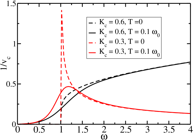
Figure 6: (Color online) Frequency dependence of ${\rm Im}\chi_{i}^{R,4k_{F}}(k_{\pm}=1,\omega)$, Eq. (IV.1.3), for various interaction strengths $K_{c}$ and temperatures $T$. The charge velocity is fixed at $v_{c}=1$. At $K_{c}=0.5$ there is a crossover from a sharp peak for $K_{c}<0.5$ at $\omega=k_{\pm}$ to monotonically increasing (with $\omega$) threshold-type behavior for $K_{c}>0.5$. Finite temperature acts to smear the $T=0$ $\omega=k_{\pm}$ singularity and adds weight to ${\rm Im}\chi_{i}^{R,4k_{F}}(k_{\pm}=1,\omega)$ for $\omega<k_{\pm}$.

The temperature dependence of ${\rm Im}\chi_{i}^{R,4k_{F}}(k_{\pm}=1,\omega)$ for different interaction values $K_{c}$ is shown in Fig. 6. At $K_{c}=0.5$ there is a crossover from a divergence to a threshold-type behavior. The main effect of the temperature is to smooth the sharper features near $\omega=v_{c}k$.

IV.2 Weakly Disordered Wires

IV.2.1 Slowly varying background potential

Modulation doping in quantum wire systems gives rise to a smoothly varing background potential. Such disorder has an important effect on the drag as it impacts the nature of the electronic states that participate in drag.Gornyi et al. (2005) Since the coupling of the density to the potential depends crucially on the Fourier components $k$, there is an important difference in how the charge density couples to disorder in the spin coherent and spin incoherent regimes. Consider the following coupling of the density to background potential modulations:

$$H_{\rm dis}=\int dxV(x)\rho(x)\hskip 142.26378pt$$

$$\approx\int dx\biggl{[}V_{0}(x)\rho_{0}(x)+V_{2k_{F}}(x)\rho_{2k_{F}}(x)+V_{4k_{F}}(x)\rho_{4k_{F}}(x)\biggr{]}.$$

Here $V_{2k_{F}}(x)={\rm Re}[V_{2k_{F}}e^{i2k_{F}x}]$ and $V_{4k_{F}}(x)={\rm Re}[V_{4k_{F}}e^{i4k_{F}x}]$. We can study the scaling dimensions of $V_{2k_{F}},V_{4k_{F}}$ using the expression for the density, Eq. (III.1.2), after integrating out the high energy field $u_{\pi}$ in favor of the lower energy spin fields. The scaling dimensions of the different scattering terms can then be determined from the action (where the integration over $x$ has already been caried out)

$$S_{\rm dis}^{2k_{F}}\sim\int d\tau V_{2k_{F}}e^{i\sqrt{2}\theta_{c}}e^{i\sqrt{2}\theta_{s}}+h.c.\;,$$ (50)

and

$$S_{\rm dis}^{4k_{F}}\sim\int d\tau V_{4k_{F}}e^{i\sqrt{8}\theta_{c}}+h.c.\;,$$ (51)

which gives

$${\rm dim}[V_{2k_{F}}]=1-\frac{K_{c}}{2}-\frac{K_{s}}{2},$$ (52)

$${\rm dim}[V_{4k_{F}}]=1-2K_{c}.$$ (53)

In these units $SU(2)$ invariance implies $K_{s}=1$, so that the $2k_{F}$ piece is more relevant than the $4k_{F}$ piece of the potential whenever $K_{c}>1/3$. Thus, we expect to see strong temperature dependence of the pinning of the density whenever $K_{c}>1/3$ as the more relevant $2k_{F}$ piece will be lost for $T\gg J_{0}$. Moreover, if $1/2<K_{c}<1$ the $2k_{F}$ piece is relevant while the $4k_{F}$ piece is irrelevant. In this case, the effect should be most dramatic. The regime $1/2<K_{c}<1$ can be reached for large but finite $U$ in a one dimensional Hubbard model.

IV.2.2 Effects of random correlations in forward scattering on the correlation functions

As the $k\approx 0$ part of the back ground potential fluctuations are often the most important at low energies, it is worthile to reviewVoit (1995) their influence on the density-density correlation function. The forward scattering part of the background potential is

$$H_{\rm dis}^{f}=\int dxV_{0}(x)\rho_{0}(x)=-\frac{\sqrt{2}}{\pi}\int dxV_{0}(x)\partial_{x}\theta_{c}(x)\;,$$ (54)

where we have we have used the result (III.1.2) and assumed $\int dxV_{0}(x)\rho_{0}=0$. Forward scattering can be completely eliminated from the Hamiltonian (action) by making the change of variables

$$\tilde{\theta}_{c}(x)=\theta_{c}(x)-\frac{\sqrt{2}K_{c}}{v_{c}}\int^{x}\!\!\!dzV_{0}(z)\;,$$ (55)

and completing the square in Eq.(III.1.1). Assuming that the disorder has white noise correlations given by the distribution $P_{V_{0}}={\rm exp}[-D^{-1}\int dz|V_{0}(z)|^{2}]$,

$$\overline{V_{0}(x)V_{0}(x^{\prime})}=\frac{D}{2}\delta(x-x^{\prime})\;,$$ (56)

where the overbar indicates a disorder average, and the constant $D\sim v_{c}/\tau_{\rm scatt}$ with $\tau_{\rm scatt}$ the typical scattering time for the electrons. The disorder averaged parts of the density-density correlation function can then readily be determined:

$$\overline{\langle[\rho_{0}^{\rm eff}(x,t),\rho_{0}^{\rm eff}(0,0)]\rangle}=\langle[\rho_{0}^{\rm eff}(x,t),\rho_{0}^{\rm eff}(0,0)]\rangle|_{V_{0}=0},$$ (57)

$$\overline{\langle[\rho_{2k_{F}}^{\rm eff}(x,t),\rho_{2k_{F}}^{\rm eff}(0,0)]\rangle}=\hskip 85.35826pt$$

$$e^{-D\left(K_{c}\over v_{c}\right)^{2}|x|}\langle[\rho_{2k_{F}}^{\rm eff}(x,t),\rho_{2k_{F}}^{\rm eff}(0,0)]\rangle|_{V_{0}=0},$$ (58)

$$\overline{\langle[\rho_{4k_{F}}^{\rm eff}(x,t),\rho_{4k_{F}}^{\rm eff}(0,0)]\rangle}=\hskip 85.35826pt$$

$$e^{-4D\left(K_{c}\over v_{c}\right)^{2}|x|}\langle[\rho_{4k_{F}}^{\rm eff}(x,t),\rho_{4k_{F}}^{\rm eff}(0,0)]\rangle|_{V_{0}=0}.$$ (59)

It is evident that larger wavevectors are suppressed more by the forward scattering with no suppression at all for the $k\approx 0$ part of the density. Treating the $2k_{F}$ and $4k_{F}$ backscattering contributions with white noise correlations analogous to (56) is more involved and requires studying renormalization group flows.Giamarchi and Schulz (1988) However, we reiterate that if the disorder is slowly-varying (as expected from donor potential modulations in modulation doped structures), the $2k_{F}$ and $4k_{F}$ potentials are relatively weak and probably negligible, at least in the sorts of structures optimized for the drag measurements we envision here!

IV.2.3 Fourier transform of disorder averaged correlation functions

Once the Fourier transforms of the $2k_{F}$ and $4k_{F}$ density-density correlation functions (IV.1.2) and (IV.1.3) are known, the Fourier transforms of the disorder averaged correlation functions are readily computed from the convolution theorem

$$\overline{{\rm Im}\chi^{R}_{i}(k,\omega)}=\int_{-\infty}^{\infty}\frac{dq}{2\pi}\frac{2l^{-1}}{l^{-2}+(k-q)^{2}}{\rm Im}\chi^{R}_{i}(q,\omega)\;,$$ (60)

where $l^{-1}=D(K_{c}/v_{c})^{2}$ for the $2k_{F}$ pieces and $l^{-1}=4D(K_{c}/v_{c})^{2}$ for the $4k_{F}$ pieces. The main effect of the disorder is thus to broaden the singularities in $\chi^{R}_{i}(k,\omega)$ by an amount of order $l^{-1}$ in momentum space. Hence, the $4k_{F}$ singularities are broadened 4 times as much as the $2k_{F}$ singularities.

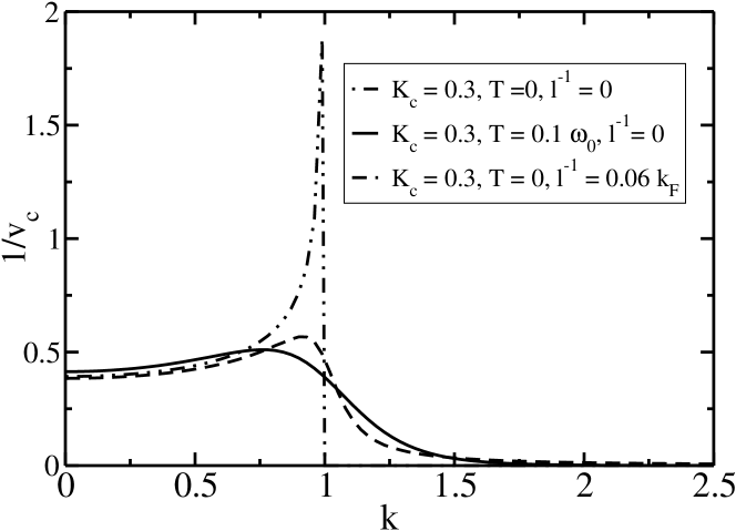
Figure 7: Disorder and thermal broadening of ${\rm Im}\chi^{R,4k_{F}}_{i}(k,\omega=1)$. The charge velocity is fixed at $v_{c}=1$. The disorder broadening is computed using Eq. (60). The effects of weak forward scattering on the $4k_{F}$ density fluctuations are qualitatively similar to that of thermal broadening–see case of $l=0.06\,k_{F}$. Analagous results are also obtained for the $2k_{F}$ density fluctuations.

Fig. 7 illustrates the effect of weak disorder on ${\rm Im}\chi^{R,4k_{F}}_{i}(k,\omega)$. Qualitatively the effects of disorder are very similar to finite temperature–there is a broadening of the sharpest features in the response. This has implications for the temperature dependence of the drag as we discuss in the next section.

V Study of the Coulomb Drag

We have already discussed several features of the drag in the previous sections of this paper, including the temperature dependence (in certain limits) of the $k\approx 2k_{F}$ and $k\approx 4k_{F}$ contributions to the drag. Implicit in those discussions was that the wires were identical. In this section we will present numerical calculations of the Coulomb drag as a function of temperature for identical and non-identical wires, and attempt to illuminate the crossover to the spin incoherent regime with semi-quantitative estimates.

V.1 Drag at low temperatures and in the crossover to the spin incoherent regime

V.1.1 The low temperature Luttinger liquid regime

At the lowest temperatures where $T\ll J_{0}$ we showed that the low energy theory (III.1.1), (22) results in the following temperature dependence of the drag resistivity (7)

$$r_{D}\approx A(K_{c},v_{c})(4k_{F})^{2}\tilde{U}^{2}_{12}(4k_{F})\left(\frac{T}{T_{4k_{F}}}\right)^{8K_{c}-3}\hskip 28.45274pt$$

$$+B(K_{c},K_{s},v_{s}/v_{c})(2k_{F})^{2}\tilde{U}^{2}_{12}(2k_{F})\left(\frac{T}{T_{2k_{F}}}\right)^{2(K_{c}+K_{s})-3}$$ (61)

where $A(K_{c},v_{c})$ and $B(K_{c},K_{s},v_{s}/v_{c})$ are functions that depend on the variables indicated and $T_{2k_{F}}^{-1}=\pi\alpha/\sqrt{v_{c}v_{s}}$ and $T_{4k_{F}}^{-1}=\pi\alpha/v_{c}$ are effective temperatures in the respective sectors. It is evident from (V.1.1) that the temperature dependence of the $k\approx 2k_{F}$ and $k\approx 4k_{F}$ contributions are different so there is a temperature at which the two balance out:

$$\frac{T^{**}}{T_{2k_{F}}}=\left[\left(\frac{T_{4k_{F}}}{T_{2k_{F}}}\right)^{8K_{c}-3}\frac{B(K_{c},K_{s},v_{s}/v_{c})\tilde{U}^{2}_{12}(2k_{F})}{4A(K_{c},v_{c})\tilde{U}^{2}_{12}(4k_{F})}\right]^{\frac{1}{6K_{c}-2K_{s}}},$$ (62)

From here on, we will assume $SU(2)$ symmetry which implies $K_{s}=1$. When $K_{s}=1$ it is clear that the $2k_{F}$ contribution to the drag is an increasing function of temperature whenever $K_{c}>1/2$ and a decreasing function otherwise. For the $4k_{F}$ contribution the boundary between increasing and decreasing contributions is $K_{c}=3/8$. Finally, by comparing the exponents of the $2k_{F}$ and $4k_{F}$ terms, one finds that the $4k_{F}$ pieces dominate the drag for $K_{c}>1/3$ when $T>T^{**}$, while the $2k_{F}$ pieces dominate the drag for $K_{c}<1/3$ in the same temperature regime. Note that this implies that the $2k_{F}$ density oscillations are more important for the drag at higher temperatures when the interactions are strong enough that $K_{c}<1/3$. This requires, of course, that the system is still at low enough temperatures that the spin degrees of freedom can be described by the effective low energy theory (22). In order to obtain $T^{**}<J_{0}$ and for the analysis above to be reasonable, we expect that we must have $\tilde{U}(2k_{F})\gg\tilde{U}(4k_{F})$.

From the results of Appendix C we can express the ratio

$$\frac{B(K_{c},K_{s},v_{s}/v_{c})}{A(K_{c},v_{c})}=\left(\frac{J_{1}}{16\pi m\omega_{0}^{2}a^{2}}\right)^{4}\frac{I_{2k_{F}}(K_{c},K_{s},v_{s}/v_{c})}{I_{4k_{F}}(K_{c})},$$ (63)

where $I_{2k_{F}}(K_{c},K_{s},v_{s}/v_{c})$ and $I_{4k_{F}}(K_{c})$ are given by Eqs. (101) and (102). As $v_{s}/v_{c}\to 0$ the crossover temperature (62) becomes very small because both $I_{2k_{F}}(K_{c},K_{s},v_{s}/v_{c})\ll I_{4k_{F}}(K_{c})$ and $\left(\frac{J_{1}}{16\pi m\omega_{0}^{2}a^{2}}\right)^{4}\sim\left(\frac{v_{s}}{v_{c}}\right)^{4}\ll 1$ in that limit. Of course, as $v_{s}$ shrinks for fixed $v_{c}$, the temperature range over which the LL theory itself is valid is also shrinking and the spin incoherent regime (where only the $4k_{F}$ density modulations remain) is approached.

V.1.2 Crossover to the spin incoherent regime

The hallmark of the spin incoherent regime is the equivalence of the real electron system with spin to a spinless systemFiete et al. (2005b) with the exception of the Green’s functionFiete and Balents (2004) and other non-particle conserving operators. In the case of drag, spin incoherence manifests itself as a thermal washing out of the $2k_{F}$ oscillations in the density-density correlation function (II). When the interactions are as strong as they are here, the weight of the $2k_{F}$ oscillations are already down by a factor $\sim\left(\frac{J_{1}}{16\pi m\omega_{0}^{2}a^{2}}\right)^{2}$ even at zero temperature.

As we have discussed before,Fiete and Balents (2004) the spin incoherent regime can be understood by starting with $T\gg J_{0}$, taking $J_{0}\to 0$, for fixed $T$ and then finally taking $T\to 0$. In the present formulation this is equivalent to fixing a finite, but low temperature, applying the low energy theory (III.1.1) and (22) and then taking the limit $v_{s}/v_{c}\to 0$ as we did in the previous section. The approach to the spin incoherent drag regime can be directly obtained via this procedure. One expects that as $v_{s}$ is lowered, the power law (40) will first breakdown (at temperatures it once held for larger $v_{s}$) before the contribution vanishes altogether from $f(T/J_{0})$.

V.2 Drag in the spin incoherent regime

In this subsection we present some numerical results justifying earlier analytical arguments for the temperature dependence of the drag. We first consider identical wires and then we study non-identical wires.

V.2.1 Identical Wires

When the wires are identical we expect the temperature dependence of the Coulomb drag given in Eq. (V.1.1) to be obtained at the lowest energies. However, as we have seen in the previous sections the $2k_{F}$ oscillations are rapidly washed out in the limit $v_{s}/v_{c}\to 0$ and only the $4k_{F}$ oscillations remain. In this subsection, we provide numerical evidence that the manipulations leading to the $4k_{F}$ temperature dependence of (V.1.1) is justified. Since these are also the same arguments leading to the $2k_{F}$ temperature dependence of $r_{D}$ at the lowest temperature, these are implicitly justified as well. Fig. 8 illustrates the comparison between the exact result from (IV.1.3) substituted into (7), and the approximate power law (46). A disorder value of $l^{-1}=0.13k_{F}$ was used in Eq. (60) to compute the drag of the disordered system from Eq. (7). The drag was computed over a temperature range $0.01\omega_{0}\leq T\leq 0.5\omega_{0}$. For $k_{B}T\gg\hbar v_{c}/l$ the drag of the clean and disordered system are indistinguishable, while for $k_{B}T\ll\hbar v_{c}/l$ there is a crossover of the temperature dependence to another power of the temperature. Empirically, we found the power law

$$r_{D}^{4k_{F},\rm disorder}\propto T^{8K_{c}-2}$$ (64)

to be a very good fit for any value of $0<K_{c}<1$. This temperature dependence can actually be inferred from (IV.1.3), (7) and Fig. 6. As we have argued several times earlier, the $\omega$ integration in (7) does not contribute any temperature dependence beyond the $(T^{4K_{c}-2})^{2}$ factors in front of $\eqref{eq:chi_4kF_int}$ (with the square coming from the drag formula (7)). When $k_{B}T\ll\hbar v_{c}/l$, the $k$ integration picks up a contribution proportional to $T^{2}$ rather than $T$. Adding up the exponents leads to $r_{D}^{4k_{F},\rm disorder}\propto T^{8K_{c}-2}$.

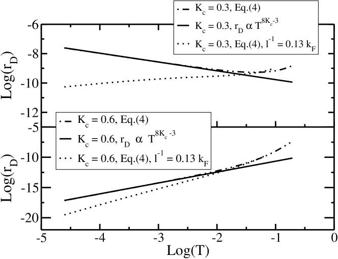
Figure 8: Temperature dependence of the Coulomb drag in the spin incoherent regime where only the $4k_{F}$ components of the density fluctuations contribute. The drag was computed over a temperature range $0.01\omega_{0}\leq T\leq 0.5\omega_{0}$. Shown is a comparison between the drag formula (7) with (IV.1.3) substituted in and the approximate power law (46). Two values of the interaction parameter $K_{c}$ are shown. A disorder value of $l^{-1}=0.13k_{F}$ was used in Eq. (60) to compute the drag from Eq. (7). For $k_{B}T\gg\hbar v_{c}/l$ the drag for the clean and disordered system are indistinguishable, while for $k_{B}T\ll\hbar v_{c}/l$ there is a crossover of the temperature dependence to another power of the temperature. Empirically, we found the power law $r_{D}^{4k_{F},\;\rm disorder}\propto T^{8K_{c}-2}$ to be a very good fit for any value of $0<K_{c}<1$.

V.2.2 Drag for non-identical wires

Coulomb drag for non-identical wires and the incommensurate-commensurate transition has been discussed for fully coherent clean wires in Ref. Fuchs et al., 2005. Via the mapping detailed in Ref. Fiete et al., 2005b the incommensurate-commensurate transition can be ready discussed deep in the spin incoherent regime. In Fig. 9 we present some numerical results for the dependence of the drag for small density mismatches between the two wires. Note that weaker interactions and higher temperatures lead to a more robust drag effect between two wires of slightly different densities. Note also that with only a few percent change in the relative densities of the wires the drag effect is substantially reduced.

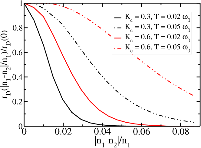
Figure 9: (Color online) Coulomb drag dependence on relative wire density at fixed temperature. We have set $v_{c}=1$. The Coulomb drag between two wires drops rapidly as a function of density mismatch. Only a few percent change in the relative densities of the wires results in a dramatic suppression of the drag. At higher temperatures and weaker interactions the drag response is more robust to small density differences between the wires.

The effects of disorder on the drag for density mismatched wires is shown in Fig. 10. When $\hbar v_{c}/l\gtrsim k_{B}T$ the disorder has a significant effect–making the drag more robust for non-identical wires. While for small $|n_{1}-n_{2}|$ the drag is reduced relative to the clean limit, for larger $|n_{1}-n_{2}|$ there can be appreciable enhancement.

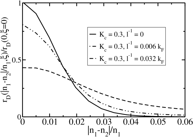
Figure 10: Coulomb drag dependence on relative wire density at fixed temperature for different values of disorder. Here $T=0.02\,\omega_{0}$ and $v_{c}=1$. While for clean wires the Coulomb drag drops rapidly as a function of density mismatch, some amount of residual disorder allows for a more robust drag effect between quantum wires that may have slightly different values of $k_{F}$.

Finally, we note that in the case of clean wires of different charge velocities but the same Fermi wavevector (in which case the $K_{c}$ are diffferent) the temperature dependence of the drag is

$$r_{D}^{4k_{F}}\sim T^{4(K_{c,1}+K_{c,2})-3}\;,$$ (65)

and if the temperature is also much less than $J_{0}$,

$$r_{D}^{2k_{F}}\sim T^{K_{c,1}+K_{c,2}+K_{s,1}+K_{s,2}-3}\;.$$ (66)

VI Summary of Results

We have discussed the Coulomb drag between two quantum wires in the limit of low electron density where at finite temperatures the energy hierarchy $J\ll T\ll E_{F}$ can be obtained.Ste In this limit, the spin degrees of freedom are completely incoherent and we have shown this implies the loss of $2k_{F}$ oscillations in the density-density correlation function. As a result, a non-monotonic temperature dependence of the drag on temperature may result. In the spin incoherent Luttinger liquid regime, the drag problem maps onto the identical problem for a spinless Luttinger liquid only with $K_{c-}\to 2K_{c-}$ so that for a clean wire the drag resistivity goes as $\rho_{D}\propto T^{8K_{c-}-3}$, where $K_{c-}$ is the coupling parameter of the antisymmetric charge mode of a Luttinger liquid theory with spin. We have shown this temperature dependence explicitly with approximate analytical calculations and confirmed those approximations with numerics.

Our results are based on a fluctuating Wigner solid model appropriate to quantum wires in a very strongly interacting regime, which typically implies low electron density. The spin sector is modeled as a nearest-neighbor antiferromagnetic Heisenberg spin chain. Without any coupling of the spin and charge sectors, no $2k_{F}$ density modulations appear. However, including a magneto-elastic coupling term that allows for a linear change in the nearest-neighbor spin coupling for small distortions induces $2k_{F}$ oscillations in the density. The coupling is weak, however, and the $2k_{F}$ oscillations are easily washed out by temperatures $T\gtrsim J$.

The fluctuating Wigner solid model is studied by deriving effective expressions for the density operator when the highest energy phonon modes are integrated out in favor of spin operators. At the lowest energies (including the spin energy) an expression is obtained equivalent to that known well in Luttinger liquid theory except the $2k_{F}$ terms contain a prefactor of order the ratio of kinetic to potential energy. Nevertheless, in this limit all correlations functions exhibit power law decay with the familiar exponents of the spin and charge sectors.

These density operators are then used to compute density-density correlation functions which are Fourier transformed into frequency and momentum space and used in previously derived drag formulas. Since the density operator has contributions at momenta $k\approx 0,\;k\approx 2k_{F}$, and $k\approx 4k_{F}$ the Coulomb drag will generically contain contributions from each of these pieces. We show explicitly that the $k\approx 0$ piece vanishes due to the harmonic approximation to the Wigner solid. This is equivalent to linearizing the electron dispersion in the standard Luttinger liquid treatment for weakly interacting electrons. Generically, the $k\approx 2k_{F}$ and $k\approx 4k_{F}$ contributions are non-vanishing and we explicitly compute their temperature dependence, $T^{2K_{c}-1}e^{-cT/J_{0}}$ and $T^{8K_{c}-3}$, in the low temperature regimes.

We have also considered the case of non-ideal wires in which weak disorder is present. We find that white-noise correlated forward scattering disorder does not affect the $k\approx 0$ result, while it tends to broaden the sharp $k-$space features of the $k\approx 2k_{F}$ and $k\approx 4k_{F}$ density-density correlation function in a manner similar to temperature. As a result, the drag resistivity crosses over to a different power law, $T^{2K_{c}}$ and $T^{8K_{c}-2}$, which is increase by one power of the temperature relative to the clean result. Finally, we have also studied the reduction of the drag due to a density mismatch between the two wires and shown the drag may be substantially reduced with only a few percent change in the relative densities of the wires. When disorder is present the drag is more robust to density mismatches between the two wires and this fact is likely to play an important role in real drag experiments.

We hope that this work will help to inspire further experimental studies on one-dimensional drag, which to date is quite limited.

Appendix A Exact expressions for $\langle\rho(x,\tau)\rho(x^{\prime},\tau^{\prime})\rangle$ up to second order in $J_{1}$

The low-energy description given in Sec. III can be treated more accurately, but in a less physically transparent way by applying the results of this appendix.

A.1 Diagonalization of $H_{c}$

The charge Hamiltonian (12) is diagonalized by the transformation

$$u_{l} = \frac{1}{\sqrt{N}}\sum_{k}e^{ikal}u_{k}\;,$$ (67)

$$p_{l} = \frac{1}{\sqrt{N}}\sum_{k}e^{-ikal}p_{k}\;,$$ (68)

(assuming periodic boundary conditions) where the theory is quantized by imposing $[u_{l},p_{m}]=i\hbar\delta_{lm}$ and $[u_{k},p_{k^{\prime}}]=i\hbar\delta_{kk^{\prime}}$. Making these substitutions we find

$$H_{c}=\sum_{k=k_{1}}^{k_{N}}\frac{p_{k}p_{-k}}{2m}+\frac{m\omega_{k}^{2}}{2}u_{k}u_{-k}\;,$$ (69)

where $\omega_{k}=2\omega_{0}|\sin\left(\frac{ka}{2}\right)|\approx v_{c}|k|$ for small $k$ with $v_{c}=\omega_{0}a$ the sound velocity of the charge modes. In momentum space the harmonic chain is just a sum of harmonic oscillators with frequencies that depend on the wavenumber $k$.

The Hamiltonian (69) can be brought into a particularly simple form via the transformation

$$a_{k} = \sqrt{\frac{m\omega_{k}}{2\hbar}}\left(u_{k}+\frac{i}{m\omega_{k}}p_{-k}\right)\;,$$ (70)

$$a^{\dagger}_{k} = \sqrt{\frac{m\omega_{k}}{2\hbar}}\left(u_{-k}-\frac{i}{m\omega_{k}}p_{k}\right)\;,$$ (71)

which brings $H_{c}$ to

$$H_{c}=\sum_{k}\hbar\omega_{k}\left(n_{k}+\frac{1}{2}\right)\;.$$ (72)

For later reference it is useful to note that

$$u_{l}(t)=\sum_{k}M_{k}(l)\left(a_{k}e^{-\omega_{k}\tau}+a^{\dagger}_{-k}e^{\omega_{k}\tau}\right)\;,$$ (73)

where $M_{k}(l)\equiv\sqrt{\frac{\hbar}{2Nm\omega_{k}}}e^{ikal}$ and we have used $\omega_{k}=\omega_{-k}$.

A.2 Notation for perturbation theory

The general expression for the density-density correlation function at finite temperature $T=1/\beta$ is

$$\langle\rho(x,\tau)\rho(x^{\prime},\tau^{\prime})\rangle=\frac{\langle U(\beta)\rho(x,\tau)\rho(x^{\prime},\tau^{\prime})\rangle_{0}}{\langle U(\beta)\rangle_{0}}\;,$$ (74)

where

$$U(\beta)=\sum_{n=0}^{\infty}(-1)^{n}\int_{0}^{\beta}d\tau_{1}...\int_{0}^{\tau_{n-1}}\hat{H}^{\prime}(\tau_{1})...\hat{H}^{\prime}(\tau_{n})\;,$$ (75)

with the operators taken in the interaction representation. The averages $\langle...\rangle_{0}\equiv{\rm Tr}[e^{-\beta H_{0}}...]$ where the $0^{th}$ order Hamiltonian is (16) taken with $J_{1}\equiv 0$:

$$H_{0}=H_{c}+J_{0}\sum_{l}{\vec{S}_{l+1}}\cdot{\vec{S}_{l}}\;,$$ (76)

and $H^{\prime}$ is the correction to this to be treated in perturbation theory

$$H^{\prime}=J_{1}\sum_{l}(u_{l+1}-u_{l}){\vec{S}_{l+1}}\cdot{\vec{S}_{l}}\;.$$ (77)

A.3 Evaluation of the density-density correlation function

A.3.1 Zeroth Order

At zeroth order we have $J_{1}\equiv 0$ and there is no coupling between the charge and the spin degrees of freedom. Therefore we can completely ingore the spin sector since it traces out trivially. Thus,

$$\langle\rho(x,\tau)\rho(x^{\prime},\tau^{\prime})\rangle^{(0)}=Z_{c}^{-1}{\rm Tr}[e^{-\beta H_{c}}\rho(x,\tau)\rho(x^{\prime},\tau^{\prime})]\;,$$ (78)

where $Z_{c}={\rm Tr}[e^{-\beta H_{c}}]$ is the partition function of the charge sector and the density is expressed as $\rho(x,\tau)=\sum_{l=1}^{N}\delta(x-al-u_{l}(\tau))$. From the Hamiltonian (72) $Z_{c}$ can be readily evaluated as

$$Z_{c}=\prod_{k}\sum_{n_{k}=0}^{\infty}e^{-\beta\hbar\omega_{k}(n_{k}+1/2)}=\prod_{k}e^{-\beta\hbar\omega_{k}/2}\frac{1}{1-e^{-\beta\hbar\omega_{k}}}\;,$$ (79)

which we will make use of later. Thus,

$$\langle\rho(x,\tau)\rho(x^{\prime},\tau^{\prime})\rangle^{(0)}=Z_{c}^{-1}\sum_{l,l^{\prime}}\int\frac{d\eta}{2\pi}\frac{d\xi}{2\pi}e^{i\eta(x-al)}e^{i\xi(x^{\prime}-al^{\prime})}$$

$$\times{\rm Tr}\left[e^{-\beta H_{c}}e^{-i\eta u_{l}(\tau)}e^{-i\xi u_{l^{\prime}}(\tau^{\prime})}\right],\hskip 28.45274pt$$ (80)

where the quantities $u_{l}$ appearing in the exponent of the trace can be expressed using Eq. (73). Using $e^{A+B}=e^{A}e^{B}e^{-[A,B]/2}$ (where $[A,B]$ commutes with both $A$ and $B$ separately), we focus on the trace and obtain

$${\rm Tr}[e^{-\beta H_{c}}e^{-i\eta u_{l}(\tau)}e^{-i\xi u_{l^{\prime}}(\tau^{\prime})}]=e^{-\frac{1}{2}\sum_{q}|M_{q}|^{2}(\eta^{2}+\xi^{2})}$$

$$\times e^{-\eta\xi\sum_{q}|M_{q}|^{2}e^{iqa(l-l^{\prime})-\omega_{q}(\tau-\tau^{\prime})}}$$

$$\times \prod_{k}{\rm Tr}^{(k)}\left[e^{-\beta\hbar\omega_{k}(a^{\dagger}_{k}a_{k}+1/2)}e^{-iC^{*}(k)a^{\dagger}_{k}}e^{-iC(k)a_{k}}\right],$$

where $C(k)\equiv|M_{k}|(\eta e^{ikal-\omega_{k}\tau)}+\xi e^{ikal^{\prime}-\omega_{k}\tau^{\prime})})$. Evaluating the trace for each $k$ independently and using definition of a Laguerre polynomial of order $n_{k}$,

$$L_{n_{k}}(-|C(k)|^{2})\equiv\langle n_{k}|e^{-iC^{*}(k)a^{\dagger}_{k}}e^{-iC(k)a_{k}}|n_{k}\rangle\;,$$ (82)

and then applying the important formula

$$\sum_{n=0}^{\infty}L_{n}(|C|^{2})z^{n}=\frac{1}{1-z}{\rm exp}\left\{|C|^{2}\frac{z}{z-1}\right\}\;,$$ (83)

we find

$$\langle\rho(x,\tau)\rho(x^{\prime},\tau^{\prime})\rangle^{(0)}=\sum_{l,l^{\prime}}\int\frac{d\eta}{2\pi}\frac{d\xi}{2\pi}e^{i\eta(x-al)}e^{i\xi(x^{\prime}-al^{\prime})}$$

$$\times e^{-\frac{1}{2}F(\eta^{2}+\xi^{2})}e^{-\eta\xi G(l,l^{\prime})}\;,\hskip 17.07182pt$$ (84)

where

$$F\equiv\sum_{q}|M_{q}|^{2}\biggl{[}1+\frac{2e^{-\beta\hbar\omega_{q}}}{1-e^{-\beta\hbar\omega_{q}}}\biggr{]}\;,$$ (85)

and

$$G(l,l^{\prime})\equiv\sum_{q}|M_{q}|^{2}\biggl{[}e^{i\theta_{q}(l,l^{\prime};t,t^{\prime})}+\frac{2\cos\left(\theta_{q}(l,l^{\prime};t,t^{\prime})\right)e^{-\beta\hbar\omega_{q}}}{1-e^{-\beta\hbar\omega_{q}}}\biggr{]}\;,$$ (86)

and $\theta_{q}(l,l^{\prime};t,t^{\prime})=qa(l-l^{\prime})-\omega_{q}(t-t^{\prime})$, where $t=-i\tau$. Finally, shifting the summation variables $\tilde{l}=l-l^{\prime}$ and performing the integrations we obtain

$$\langle\rho(x,t)\rho(x^{\prime},t^{\prime})\rangle^{(0)}$$

$$= \frac{1}{a}\sum_{l}\frac{1}{2\pi}\sqrt{\frac{\pi}{F-G(l)}}{\rm exp}\left\{-\frac{(x-x^{\prime}-al)^{2}}{4(F-G(l))}\right\},$$

where

$$F-G(l)=\frac{a\hbar}{mv_{c}2\pi}\Biggl{[}\ln\biggl{[}\frac{\alpha^{2}+(al)^{2}+(v_{c}(\tau-\tau^{\prime}))^{2}}{\alpha^{2}}\biggr{]}$$

$$+2\sum_{n=0}^{\infty}\ln\biggl{[}\frac{(\alpha+(n+1)\beta\hbar v_{c})^{2}+(al)^{2}+(v_{c}(\tau-\tau^{\prime}))^{2}}{(\alpha+(n+1)\beta\hbar v_{c})^{2}}\biggr{]}\Biggr{]}.$$

Here $\alpha$ is a short distance cut off of order the lattice spacing $a$. Note that for finite temperatures the second sum is cut off when the argument of the $\ln$ becomes ${\cal O}(1)$ which occurs when $n=n_{l}\sim\sqrt{(al)^{2}+(v_{c}(\tau-\tau^{\prime}))^{2}}/(\beta\hbar v_{c})$. In the limit of $T\to 0$, $\beta\to\infty$ and the second terms drops out all together. In this paper we are interested in the limit $T\ll E_{F}$, so the second term can be ignored altogether. We will not explicitly consider finite temperatures in the first and second order expressions.

A.3.2 First order

The manipulations needed here are identical to those used to compute the zeroth order result, so we simply quote the result:

$$\langle\rho(x,\tau)\rho(x^{\prime},\tau^{\prime})\rangle^{(1)}=J_{1}N\sum_{n}\int_{0}^{\beta}d\tilde{\tau}\langle{\vec{S}_{l+1}}\cdot{\vec{S}_{l}}(\tilde{\tau})\rangle^{(0)}$$

$$\times\frac{I(n)}{2\pi a}\prod_{k>0}^{k_{\rm max}}|M(k)|^{4}4(1-\cos(ka))$$

$$\times(1-\cos\left(\theta_{k}(n,0;\tau,\tau^{\prime})\right))e^{-2\tilde{\tau}\hbar\omega_{k}},$$

where $l$ is arbitrary, $N$ is the number of electrons in the system, and

$$I(n)=e^{\frac{B^{2}}{4A}}\sum_{j=0}^{N}\frac{\sqrt{\pi}(-1)^{j}(2N)!}{(2j)!(2N-2j)!}\left(\frac{B}{2A}\right)^{2(N-j)}$$

$$\times\frac{(2j-1)!!}{2^{j}}A^{-\frac{1}{2}-j}\;,$$ (90)

where the $n$ dependence enters through $B\equiv i(x-x^{\prime}-an)$ and $A\equiv F-G(n)$. It is worth noting that neither $\langle\rho(x,\tau)\rho(x^{\prime},\tau^{\prime})\rangle^{(0)}$ nor $\langle\rho(x,\tau)\rho(x^{\prime},\tau^{\prime})\rangle^{(1)}$ contain a $2k_{F}$ component. This component will only appear in the second order term, as we now discuss.

A.3.3 Second order

The second order corrections are (where ${\bf x}=(x,\tau)$)

$$\langle\rho({\bf x})\rho({\bf x^{\prime}})\rangle^{(2)}=\int_{0}^{\beta}d\tau_{1}\int_{0}^{\tau_{1}}d\tau_{2}\frac{\langle\hat{H}^{\prime}(\tau_{1})\hat{H}^{\prime}(\tau_{2})\rho({\bf x})\rho({\bf x^{\prime}})\rangle_{0}}{Z_{c}Z_{s}}$$

$$-\langle\rho({\bf x})\rho({\bf x^{\prime}})\rangle^{(0)}\int_{0}^{\beta}d\tau_{1}\int_{0}^{\tau_{1}}d\tau_{2}\frac{\langle\hat{H}^{\prime}(\tau_{1})\hat{H}^{\prime}(\tau_{2})\rangle_{0}}{Z_{c}Z_{s}}$$

$$=(J_{1})^{2}\sum_{l,l^{\prime}}\int_{0}^{\beta}d\tau_{1}\int_{0}^{\tau_{1}}d\tau_{2}\langle{\vec{S}_{l+1}}\cdot{\vec{S}_{l}}(\tau_{1}){\vec{S}_{l^{\prime}+1}}\cdot{\vec{S}_{l^{\prime}}}(\tau_{2})\rangle^{(0)}$$

$$\times\biggl{[}\frac{\langle\hat{H}^{\prime}_{c}(l,\tau_{1})\hat{H}^{\prime}_{c}(l^{\prime},\tau_{2})\rho({\bf x})\rho({\bf x^{\prime}})\rangle_{0}}{Z_{c}}$$

$$-\langle\rho({\bf x})\rho({\bf x^{\prime}})\rangle^{(0)}\frac{\langle\hat{H}^{\prime}_{c}(l,\tau_{1})\hat{H}^{\prime}_{c}(l^{\prime},\tau_{2})\rangle_{0}}{Z_{c}}\biggr{]}\;$$

where $\hat{H}^{\prime}_{c}(l,\tau)=u_{l+1}(\tau)-u_{l}(\tau)$ is the charge part of $H^{\prime}$. From (A.3.3) it is clear that when dimer-dimer correlations $\langle{\vec{S}_{l+1}}\cdot{\vec{S}_{l}}(\tau_{1}){\vec{S}_{l^{\prime}+1}}\cdot{\vec{S}_{l^{\prime}}}(\tau_{2})\rangle^{(0)}$ are present (presumably when $T\lesssim J_{0}$) then a $2k_{F}$ component appears in $\langle\rho(x,\tau)\rho(x^{\prime},\tau^{\prime})\rangle$. After some algebra, we reach the final form

$$\langle\rho(x,\tau)\rho(x^{\prime},\tau^{\prime})\rangle^{(2)}=(J_{1})^{2}\sum_{l,l^{\prime}}\int_{0}^{\beta}d\tau_{1}\int_{0}^{\tau_{1}}d\tau_{2}$$

$$\times\langle{\vec{S}_{l+1}}\cdot{\vec{S}_{l}}(\tau_{1}){\vec{S}_{l^{\prime}+1}}\cdot{\vec{S}_{l^{\prime}}}(\tau_{2})\rangle^{(0)}$$

$$\times\sum_{n,m}\int\frac{d\eta}{2\pi}\frac{d\xi}{2\pi}e^{i\eta(x-an)}e^{i\xi(x^{\prime}-am)}$$

$$\times e^{-\frac{1}{2}\sum_{q}|M_{q}|^{2}(\eta^{2}+\xi^{2})}e^{-\eta\xi\sum_{q}|M_{q}|^{2}e^{i\theta_{q}(n,m;\tau,\tau^{\prime})}}$$

$$\times\prod_{k>0}^{k_{\rm max}}|M_{k}|^{4}4(1-\cos(ka))^{2}e^{-2(\tau_{1}-\tau_{2})\hbar\omega_{k}}$$

$$\times\biggl{(}-1+\prod_{k^{\prime}>0}^{k_{\rm max}}\Bigl{(}1+h(k^{\prime})\Bigr{)}\biggr{)}\;,$$ (92)

where

$$h(k)=|M_{k}|^{2}e^{-4\tau_{2}\hbar\omega_{k}}\Biggl{[}\eta^{2}\Biggl{(}1-\frac{e^{2\tau_{2}\hbar\omega_{k}}R(2\tilde{n})}{1-\cos(ka)}\Biggr{)}$$

$$+2\eta\xi\Biggl{(}\cos\Bigl{(}ka(l-l^{\prime})\Bigr{)}-\frac{e^{2\tau_{2}\hbar\omega_{k}}R(\tilde{n}+\tilde{m})}{1-\cos(ka)}\Biggr{)}$$

$$+\xi^{2}\Biggl{(}1-\frac{e^{2\tau_{2}\hbar\omega_{k}}R(2\tilde{m})}{1-\cos(ka)}\Biggr{)}\Biggr{]},$$ (93)

with

$$\tilde{n}=n+i\omega_{k}\tau/(ka),$$ (94)

$$\tilde{m}=m+i\omega_{k}\tau^{\prime}/(ka),$$ (95)

and

$$R(s)=\cos\Bigl{(}ka(2l^{\prime}+2-s)\Bigr{)}+\cos\Bigl{(}ka(2l^{\prime}+1-s)\Bigr{)}$$

$$+\cos\Bigl{(}ka(2l^{\prime}-s)\Bigr{)}.\hskip 22.76228pt$$ (96)

Appendix B Computing ${\rm Im}\chi_{i}^{R,0}(k,\omega)$

${\rm Im}\chi_{i}^{R,0}(k,\omega)$ is computed by making use of the Fourier expansion of $\rho^{\rm eff}_{0}(x,\tau)$, Eq. (35), and the formula (IV). Consider first the Fourier transform to momentum space:

$$\int_{-\infty}^{\infty}\!\!\!dxe^{-ikx}\langle\rho^{\rm eff}_{0}(x,\tau)\rho^{\rm eff}_{0}(0,0)\rangle=\langle\rho^{\rm eff}_{0}(k,\tau)\rho^{\rm eff}_{0}(-k,0)\rangle,$$ (97)

where translational invariance was used. The Fourier decomposition of $\rho^{\rm eff}_{0}(k,\tau)$ is readily obtained by making use of Eq. (35), the relation $u_{0}(x)/a=\sqrt{2}\theta_{c}(x)/\pi$, and the representation of $u_{0}(x)$ given in Eq. 73:

$$\rho^{\rm eff}_{0}(k,\tau)=-\frac{ik}{a}\sqrt{\frac{\hbar L}{2m\omega_{k}}}\left(a_{k}e^{-\omega_{k}\tau}+a^{\dagger}_{-k}e^{\omega_{k}\tau}\right),$$ (98)

where we have implicitly converted the discrete $k$ sums to integrals and $L$ is the length of the system. It is easily verified that this has the right units to give $\langle\rho^{\rm eff}_{0}(k,\tau)\rho^{\rm eff}_{0}(-k,0)\rangle$ in (97) the correct dimensions of inverse length. Only the expectation values of the cross terms $a_{k}a_{k}^{\dagger}$ and $a_{-k}^{\dagger}a_{-k}$ are nonzero, giving

$$\langle\rho^{\rm eff}_{0}(k,\tau)\rho^{\rm eff}_{0}(-k,0)\rangle=-\frac{k^{2}}{a^{2}}\frac{\hbar L}{2m\omega_{k}}\hskip 71.13188pt$$

$$\times\left[e^{-\omega_{k}\tau}(1+n_{B}(k))+e^{\omega_{k}\tau}n_{B}(-k)\right],$$ (99)

where $n_{B}(k)=\langle a^{\dagger}_{k}a_{k}\rangle=(e^{\beta\omega_{k}}-1)^{-1}$ is the boson occupation factor. Returning to the expression (IV) and evaluating the $\tau$ integral we find

$$\chi^{0}_{i}(k,\omega_{n})=\frac{k^{2}}{a^{2}}\frac{\hbar L}{2m\omega_{k}}\left[\frac{-1}{i\omega_{n}-\omega_{k}}+\frac{1}{i\omega_{n}+\omega_{k}}\right],$$ (100)

which upon the analytic continuation to real frequencies $i\omega_{n}\to\omega+i\eta$ leads directly to Eq. (36).

Appendix C Expressions for $I_{2k_{F}}(K_{c},K_{s},v_{s}/v_{c})$ and $I_{4k_{F}}(K_{c})$

The functions $I_{2k_{F}}(K_{c},K_{s},v_{s}/v_{c})$ and $I_{4k_{F}}(K_{c})$ defined in Eq. (63) are given by

$$I_{2k_{F}}(K_{c},K_{s},v_{s}/v_{c})=\int_{0}^{\infty}\frac{d\omega}{T}\frac{\Xi_{2k_{F}}(K_{c},K_{s},v_{s}/v_{c},\omega/T)}{\sinh^{2}(\omega/2T)},$$ (101)

and

$$I_{4k_{F}}(K_{c})=\int_{0}^{\infty}\frac{d\omega}{T}\frac{\Xi_{4k_{F}}(K_{c},\omega/T)}{\sinh^{2}(\omega/2T)},$$ (102)

where

$$\Xi_{2k_{F}}(K_{c},K_{s},v_{s}/v_{c},\omega/T)=\Biggl{(}{\rm Im}\int_{-\infty}^{\infty}\!\!\!d\tilde{x}\int_{0}^{\infty}\!\!\!d\tilde{t}e^{i\frac{\omega}{\pi T}\tilde{t}}$$

$$\times{\rm Im}\Biggl{[}\frac{1}{[\sinh(\tilde{x}-\tilde{t})\sinh(\tilde{x}+\tilde{t})]^{\frac{K_{c}}{2}}}\hskip 85.35826pt$$

$$\times\frac{1}{[\sinh\left(\tilde{x}v_{c}/v_{s}-\tilde{t}\right)\sinh(\tilde{x}v_{c}/v_{s}+\tilde{t})]^{\frac{K_{s}}{2}}}\Biggr{]}\Biggr{)}^{2},\;\;\;$$ (103)

and

$$\Xi_{4k_{F}}(K_{c},\omega/T)=\Biggl{(}{\rm Im}\int_{-\infty}^{\infty}\!\!\!d\tilde{x}\int_{0}^{\infty}\!\!\!d\tilde{t}e^{i\frac{\omega}{\pi T}\tilde{t}}$$

$$\times{\rm Im}\Biggl{[}\frac{1}{[\sinh(\tilde{x}-\tilde{t})\sinh(\tilde{x}+\tilde{t})]^{2K_{c}}}\Biggr{]}\Biggr{)}^{2}.\;\;\;$$ (104)

References

- Manoharan et al. (2000) H. C. Manoharan, C. P. Lutz, and D. M. Eigler, Nature 403, 512 (2000).
- Nygard et al. (2000) J. Nygard, D. H. Cobden, and P. E. Lindelof, Nature 408, 342 (2000).
- Jarillo-Herrero et al. (2005) P. Jarillo-Herrero, J. Kong, H. S. J. van der Zant, L. Kouwenhoven, and S. D. Francheschi, Nature 434, 484 (2005).
- Haldane (1981) F. Haldane, J. Phys. C 14, 2585 (1981).
- Voit (1995) J. Voit, Rep. Prog. Phys. 58, 977 (1995).
- Ishii et al. (2003) H. Ishii, H. Kataura, H. Shiozawa, H. Yoshioka, H. Otsubo, Y. Takayama, T. Miyahara, S. Suzuki, Y. Achiba, M. Nakatake, et al., Nature 426, 540 (2003).
- Bockrath et al. (1999) M. Bockrath, D. H. Cobden, J. Lu, A. G. Rinzler, R. E. Smalley, L. Balents, and P. L. McEuen, Nature 397, 598 (1999).
- Yao et al. (1999) Z. Yao, H. W. C. Postma, L. Balents, and C. Dekker, Nature 402, 273 (1999).
- Auslaender et al. (2002) O. M. Auslaender, A. Yacoby, R. de Picciotto, K. W. Baldwin, L. N. Pfeiffer, and K. W. West, Science 295, 825 (2002).
- Auslaender et al. (2005) O. M. Auslaender, H. Steinberg, A. Yacoby, Y. Tserkovnyak, B. I. Halperin, K. W. Baldwin, L. N. Pfeiffer, and K. W. West, Science 308, 88 (2005).
- Yamamoto et al. (2002) M. Yamamoto, M. Stopa, Y. Tokura, Y. Hirayama, and S. Tarucha, Physica E 12, 726 (2002).
- Debray et al. (2001) P. Debray, V. N. Zverev, O. Raichev, R. Klesse, P. Vasilopoulos, and R. S. Newrock, J. Phys.: Cond. Matt. 13, 3389 (2001).
- Debray et al. (2002) P. Debray, V. N. Zverev, V. Gurevich, R. Klesse, and R. S. Newrock, Semicond. Sci. Technol. 17, R21 (2002).
- Maslov and Stone (1995) D. Maslov and M. Stone, Phys. Rev. B 52, R5539 (1995).
- Safi and Schulz (1999) I. Safi and H. J. Schulz, Phys. Rev. B 59, 3040 (1999).
- Matveev (2004a) K. A. Matveev, Phys. Rev. Lett. 92, 106801 (2004a).
- Matveev (2004b) K. A. Matveev, Phys. Rev. B 70, 245319 (2004b).
- Zheng and MacDonald (1993) L. Zheng and A. H. MacDonald, Phys. Rev. B 48, 8203 (1993).
- Pustilnik et al. (2003) M. Pustilnik, E. G. Mishchenko, L. I. Glazman, and A. V. Andreev, Phys. Rev. Lett. 91, 126805 (2003).
- Fuchs et al. (2005) T. Fuchs, R. Klesse, and A. Stern, Phys. Rev. B 71, 045321 (2005).
- Klesse and Stern (2000) R. Klesse and A. Stern, Phys. Rev. B 62, 16912 (2000).
- Nazarov and Averin (1998) Y. V. Nazarov and D. V. Averin, Phys. Rev. Lett. 81, 653 (1998).
- Schlottmann (2004a) P. Schlottmann, Phys. Rev. B 69, 035110 (2004a).
- Flensberg (1998) K. Flensberg, Phys. Rev. Lett. 81, 184 (1998).
- Raichev and Vasilopoulos (2000) O. Raichev and P. Vasilopoulos, Phys. Rev. B 61, 7511 (2000).
- Raichev and Vasilopoulos (1999) O. E. Raichev and P. Vasilopoulos, Phys. Rev. Lett. 83, 3697 (1999).
- Ponomarenko and Averin (2000) V. V. Ponomarenko and D. V. Averin, Phys. Rev. Lett. 85, 4928 (2000).
- Gurevich and Muradov (2000) V. L. Gurevich and M. I. Muradov, Phys. Rev. B 62, 1576 (2000).
- Trauzettel et al. (2002) B. Trauzettel, R. Egger, and H. Grabert, Phys. Rev. Lett. 88, 116401 (2002).
- Mortensen et al. (2002) N. A. Mortensen, K. Flensberg, and A.-P. Jauho, Phys. Rev. B 65, 085317 (2002).
- Mortensen et al. (2001) N. A. Mortensen, K. Flensberg, and A.-P. Jauho, Phys. Rev. Lett. 86, 1841 (2001).
- Schlottmann (2004b) P. Schlottmann, Phys. Rev. B 70, 115306 (2004b).
- Muradov (2002) M. I. Muradov, Phys. Rev. B 66, 115417 (2002).
- Raichev (2001) O. E. Raichev, Phys. Rev. B 64, 035324 (2001).
- Cheianov and Zvonarev (2004a) V. V. Cheianov and M. B. Zvonarev, Phys. Rev. Lett. 92, 176401 (2004a).
- Cheianov and Zvonarev (2004b) V. V. Cheianov and M. B. Zvonarev, J. Phys. A: Math. Gen. 37, 2261 (2004b).
- Fiete and Balents (2004) G. A. Fiete and L. Balents, Phys. Rev. Lett. 93, 226401 (2004).
- Cheianov et al. (2005) V. V. Cheianov, H. Smith, and M. B. Zvonarev, Phys. Rev. A 71, 033610 (2005).
- Fiete et al. (2005a) G. A. Fiete, J. Qian, Y. Tserkovnyak, and B. I. Halperin, Phys. Rev. B 72, 045315 (2005a).
- Fiete et al. (2005b) G. A. Fiete, K. L. Hur, and L. Balents, Phys. Rev. B 72, 125416 (2005b).
- (41) M. Kindermann and P. W. Brouwer, cond-mat/0506455.
- (42) The relevance (in the RG sense) of tunneling in drag experiments was first pointed out by Klesse and Stern,Klesse and Stern (2000) but similar physics has also been discussed in other contexts by K. Le Hur, Phys. Rev. B 63, 165110 (2001), by Kusmart, Luther, and Nersesyan, JETP Lett. 55, 724 (1992), by Yakovenko, JETP Lett. 56, 523 (1992), and by A. O. Gogolin, A. A. Nersesyan, and A. M. Tsvelik, Bosonization and Strongly Correlated Systems (Cambridge University Press, Cambridge, England 1998).
- (43) There has been a significant amount of theoretical work done on drag in 2-d systems in recent years. See the following references and references therein: E. H. Hwang, S. Das Sarma, V. Braude, and Ady Stern, Phys. Rev. Lett. 90, 086801 (2003); S. Das Sarma and E. H. Hwang, Phys. Rev. B 71, 195322 (2005); Felix von Oppen, Steven H. Simon, and Ady Stern Phys, Rev. Lett. 87, 106803 (2001);I. V. Gornyi, A. D. Mirlin, and F. von Oppen, Phys. Rev. B 70, 245302 (2004);G. Vignale, Phys. Rev. B 71, 125103 (2005);Irene D’Amico and Giovanni Vignale, Phys. Rev. B 68, 045307 (2003).
- (44) A complementary approach to Wigner crystals in one dimension has recently been discussed by D.S. Novikov in Phys. Rev. Lett. 95, 066401 (2005) and in cond-mat/0407498.
- Glazman et al. (1992) L. I. Glazman, I. M. Ruzin, and B. I. Shklovskii, Phys. Rev. B 45, 8454 (1992).
- Häusler et al. (2002) W. Häusler, L. Kecke, and A. H. MacDonald, Phys. Rev. B 65, 085104 (2002).
- Sachdev (1999) S. Sachdev, Quantum Phase Transitions (Cambridge University Press, 1999).
- Giamarchi (2004) T. Giamarchi, Quantum Physics in One Dimension (Clarendon Press, Oxford, 2004).
- (49) S. Teber, cond-mat/0511257.
- Voit (1993) J. Voit, Phys. Rev. B 47, 6740 (1993).
- Meden and Schönhammer (1992) V. Meden and K. Schönhammer, Phys. Rev. B 46, 15753 (1992).
- Sachdev et al. (1994) S. Sachdev, T. Senthil, and R. Shankar, Phys. Rev. B 50, 258 (1994).
- Schulz (1986) H. J. Schulz, Phys. Rev. B 34, 6372 (1986).
- (54) I. S. Gradshteyn and I. M. Ryzhik, Tables of Integrals, Series, and products (Academic, New York, 1965), formula 3.312.1.
- Gornyi et al. (2005) I. V. Gornyi, A. D. Mirlin, and D. G. Polyakov, Phys. Rev. Lett. 95, 046404 (2005).
- Giamarchi and Schulz (1988) T. Giamarchi and H. J. Schulz, Phys. Rev. B 37, 325 (1988).
- (57) H. Steinberg, O. M. Auslaender, A. Yacoby, J. Qian, G. A. Fiete, Y. Tserkovnyak, B. I. Halperin, K. W. Baldwin, L. N. Pfeiffer,and K. W. West cond-mat/0506812.