First-Principles Calculations at Constant Polarization

Abstract

We develop an exact formalism for performing first-principles calculations for insulators at fixed electric polarization. As shown by Sai, Rabe, and Vanderbilt (SRV) [N. Sai, K. M. Rabe, and D. Vanderbilt, Phys. Rev. B 66, 104108 (2002)], who designed an approximate method to tackle the same problem, such an approach allows one to map out the energy landscape as a function of polarization, providing a powerful tool for the theoretical investigation of polar materials. We apply our method to a system in which the ionic contribution to the polarization dominates (a broken-inversion-symmetry perovskite), one in which this is not the case (a III-V semiconductor), and one in which an additional degree of freedom plays an important role (a ferroelectric phase of KNO₃). We find that while the SRV method gives rather accurate results in the first case, the present approach provides important improvements to the physical description in the latter cases.

In 1993 King-Smith and Vanderbilt KingSmith1993PRB introduced a theory for computing the electric polarization of an infinite solid, showing for the first time that this property was indeed a well-defined quantity for an insulating material. Their theory of the bulk polarization (TBP) is based on computing the electronic contribution to the polarization as a Berry phase of the valence-band Bloch wave functions transported across the Brillouin zone. A practical numerical scheme to compute it was given in the same paper KingSmith1993PRB , and it is now widely used in first-principles calculations. Later, Souza, Íñiguez, and Vanderbilt Souza2002PRL (SIV) used the TBP as the cornerstone for a method to calculate the exact ground state of an insulator in the presence of an electric field by minimizing an electric enthalpy functional expressed in terms of occupied Bloch-like states on a uniform grid of points in reciprocal space. It is therefore possible to compute from first-principles many interesting properties of materials related to their behavior under electric fields.

In this Letter we propose a method to do first-principles calculations not at constant electric field, but at constant electric polarization. In this way, it would become possible to map the energy $E$ of an insulator as a function of its polarization ${\bf P}$. There are several reasons why this is useful. First, it allows for a exhaustive search for competing local minima and for saddle points in a system with a complicated energy surface. These features would otherwise be hidden in a standard optimization procedure, which would only be likely to find a single miminum of the energy. Second, knowing $E({\bf P})$, we can calculate various properties related to derivatives of $E$ with respect to ${\bf P}$, such as the linear and non-linear dielectric susceptibilities. While methods of density-functional perturbation theory (DFPT) deGironcoli1989PRL_Giannozzi1991PRB_Gonze1997PRB can also be used to access these susceptibilities, our approach is advantageous in that it does not require much special-purpose programming and yields non-linear susceptibilities with very little extra effort beyond that needed to obtain the linear ones. And third, Landau-Devonshire theories have historically provided an important avenue to the understanding of ferroelectric materials, based on an expansion of the energy in powers of polarization. The ability to compute $E(\bf P)$ may open the door to the first-principles derivation of Landau-Devonshire descriptions, as opposed to the usual empirical formulations, for a wide range of ferroelectric materials.

The problem of performing simulations at constant polarization in the context of first-principles calculations has been addressed previously. In particular, Sai, Rabe, and Vanderbilt Sai2002PRB (SRV) developed an approximate method to do this and applied it to obtain $E(\bf P)$ for several perovskite systems of interest. A similar approach was used by Fu and Bellaiche to study the electromechanical response of solids under finite electric fields Fu2003PRL . Our method relies on many of the ideas of the SRV one, but it is instead an exact method because it incorporates the SIV theory of finite electric fields Souza2002PRL .

Figure 1: Sketch of energy as a function of polarization for a double-well potential. The value of the electric field needed to impose the polarization is the same at the three indicated points, as their slopes are the same.

Our goal is to find the minimum energy $E$ of a system of atoms for which the electric polarization takes some target value ${\bf P}_{\rm t}$. The system has both ionic and electronic degrees of freedom, and we will use vectors ${\bf X}$ and ${\boldsymbol{\Psi}}$ to represent them. Vector ${\bf X}$ has $3N+6$ components given by the cartesian coordinates of the $N$ atoms in the simulation cell and the 6 components of the strain tensor. On the other hand, ${\boldsymbol{\Psi}}$ contains the one-electron wave functions of the system. We are therefore facing a standard constrained optimization problem that can be solved by introducing a Lagrange multiplier ${\boldsymbol{\lambda}}$ and searching for the minimum of $E+{\boldsymbol{\lambda}}\cdot({\bf P}-{\bf P}_{\rm t})$, or, discarding the constant term, the minimum of $E+{\boldsymbol{\lambda}}\cdot{\bf P}$. Defining ${\boldsymbol{\lambda}}=-\Omega\boldsymbol{\cal{E}}$, where $\Omega$ is the volume of the unit cell of the material under consideration, we have

$$\min_{\genfrac{}{}{0.0pt}{}{{\bf X},{\boldsymbol{\Psi}}}{{\boldsymbol{\lambda}}\rightarrow{\bf P}={\bf P}_{\rm t}}}\{E({\bf X},{\boldsymbol{\Psi}})+{\boldsymbol{\lambda}}\cdot{\bf P}({\bf X},{\boldsymbol{\Psi}})\}$$

$$\quad\quad=\min_{\genfrac{}{}{0.0pt}{}{{\bf X}}{\boldsymbol{\cal{E}}\rightarrow{\bf P}={\bf P}_{\rm t}}}\{\min_{{\boldsymbol{\Psi}}}\{E({\bf X},{\boldsymbol{\Psi}})-\Omega\boldsymbol{\cal{E}}\cdot{\bf P}({\bf X},{\boldsymbol{\Psi}})\}\}$$

$$\quad\quad=\min_{\genfrac{}{}{0.0pt}{}{{\bf X}}{\boldsymbol{\cal{E}}\rightarrow{\bf P}={\bf P}_{\rm t}}}H({\bf X},\boldsymbol{\cal{E}}),$$ (1)

where ${\boldsymbol{\lambda}}\rightarrow{\bf P}={\bf P}_{\rm t}$ indicates a minimization over the values of ${\boldsymbol{\lambda}}$ that impose the constraint ${\bf P}={\bf P}_{\rm t}$. The function $H({\bf X},\boldsymbol{\cal{E}})$ is the electric enthalpy that is minimized in the SIV method to find the electronic ground-state of an insulator in the presence of an electric field $\boldsymbol{\cal{E}}$ Souza2002PRL .

Therefore, the problem of finding the minimum energy of a system that is constrained to have polarization ${\bf P}$ is equivalent to finding the ground state of a system under an electric field $\boldsymbol{\cal{E}}$ that imposes polarization ${\bf P}$. However, the apparently straightforward approach of doing calculations at different values of the electric field to find $E({\bf P})$ parametrically will not work in general. Fig. 1 illustrates why this is so for a typical double-well potential characteristic of ferroelectric perovskites. In this case, several values of the polarization correspond to the same value of the electric field, since $\boldsymbol{\cal{E}}=\Omega^{-1}(dE/d{\bf P})$, and an optimization using the SIV theory will most likely find the point that has the lowest energy of the three, i.e., the global minimum of $H(P)$. With extra care it might be possible to find the secondary local minimum of $H(P)$, but not the third solution, which is a maximum (or, in 3D, a saddle point) of $H(P)$. It follows from this line of reasoning that one cannot map the region of $E(P)$ that has negative curvature, and it may also prove difficult to map nearby regions of positive curvature.

We now describe how to perform a minimization of the enthalpy $H$ over the ionic degrees of freedom ${\bf X}$ and the electric fields $\boldsymbol{\cal{E}}$ that produce a desired polarization ${\bf P}_{\rm t}$ in a way that parallels the presentation in Sec. III.A of Ref. Sai2002PRB, . From now on, we will assume that the optimization is done while keeping the cell vectors fixed. (It is possible to remove this constraint, but it is necessary to take into account some technical subtleties related to the way in which the stress tensor is computed in the presence of an electric field. The details, together with examples, will be presented elsewhere WuIP .) We begin with a trial guess $({\bf X}_{0},\boldsymbol{\cal{E}}_{0})$, and we expand $H({\bf X},\boldsymbol{\cal{E}})$ and ${\bf P}({\bf X},\boldsymbol{\cal{E}})$ as low-order Taylor series

$$H = H_{0}-{\bf F}\,\delta{\bf X}+\frac{1}{2}\,\delta{\bf X}\,{\bf K}\,\delta{\bf X}-\Omega{\bf P}\,\delta\boldsymbol{\cal{E}},$$ (2)

$${\bf P} = {\bf P}_{0}+\frac{1}{\Omega}{\bf Z}\,\delta{\bf X}+\frac{1}{4\pi}{\boldsymbol{\chi}}\,\delta\boldsymbol{\cal{E}},$$ (3)

where $H_{0}=H({\bf X}_{0},\boldsymbol{\cal{E}}_{0})$ and ${\bf P}_{0}={\bf P}({\bf X}_{0},\boldsymbol{\cal{E}}_{0})$ (atomic units are used throughout unless stated otherwise). The $F_{i}=-(\partial H/\partial X_{i})$ are the $3N$ components of the forces on the atoms at finite electric field Souza2002PRL , the $K_{ij}=(\partial^{2}H/\partial X_{i}\partial X_{j})$ are the $3N\times 3N$ force-constant matrix elements, the $Z_{i\alpha}=\Omega(\partial P_{\alpha}/\partial X_{i})$ are the $3N\times 3$ Born effective charges, and the $\chi_{\alpha\beta}=4\pi(\partial P_{\beta}/\partial{\cal E}_{\alpha})$ are the $3\times 3$ elements of the dielectric susceptibility tensor. We can then predict that $\partial H/\partial X_{i}=0$ and ${\bf P}={\bf P}_{\rm t}$ at an ${\bf X}={\bf X}_{0}+\delta{\bf X}$ and an $\boldsymbol{\cal{E}}=\boldsymbol{\cal{E}}_{0}+\delta\boldsymbol{\cal{E}}$ given by

$$\left(\begin{array}[]{cc}{\bf K}&-{\bf Z}\\ -{\bf Z}^{T}&-\frac{\Omega}{4\pi}\,{\boldsymbol{\chi}}\end{array}\right)\left(\begin{array}[]{c}\delta{\bf X}\\ \delta\boldsymbol{\cal{E}}\end{array}\right)=\left(\begin{array}[]{c}{\bf F}\\ \Omega\Delta{\bf P}_{0}\end{array}\right),$$ (4)

where $\Delta{\bf P}_{0}={\bf P}_{0}-{\bf P}_{\rm t}$. This system of linear equations can be solved iteratively, refining $\delta{\bf X}$ and $\delta\boldsymbol{\cal{E}}$ until ${\bf F}$ and $\Delta{\bf P}_{0}$ both vanish. As mentioned before, ${\bf F}$ can be computed exactly in the presence of an electric field according to the SIV prescription Souza2002PRL . The guiding tensors ${\bf K}$, ${\bf Z}$ and ${\boldsymbol{\chi}}$ do not need to be computed exactly; replacing these by approximate versions only results in a slower convergence to the correct solution, without shifting the solution itself. In particular, we normally find it sufficient to compute ${\bf K}$, ${\bf Z}$ and ${\boldsymbol{\chi}}$ at zero electric field.

The scheme described here has been implemented to work with the ABINIT abinit density-functional theory (DFT) Hohenberg1964PR code. Instead of performing a direct iterative solution of Eq. (4), we have used a nested-loop algorithm for the sake of robustness. Starting with some guess for ${\bf X}$ and $\boldsymbol{\cal{E}}$, we keep the atoms fixed and vary the field in the internal loop until the polarization is the target one, a problem that is well behaved. Once this is achieved, we solve Eq. (4) to get new values of ${\bf X}$ and $\boldsymbol{\cal{E}}$, and iterate until convergence is achieved.

As a first example of how our method works, we apply it to a soft-mode system studied by Sai, Rabe, and Vanderbilt Sai2002PRB . They have shown that breaking the inversion symmetry in perovskites by modulating their composition in a cyclic sequence of layers produces some interesting features in their energy landscape, apart from making them promising candidates for new materials with useful piezoelectric and dielectric properties. They presented results for Ba(Ti-$\delta$, Ti, Ti+$\delta$)O₃, where the two species that alternate with Ti on the $B$ site are virtual atoms that differ from Ti in that their nucleus has an defect or excess of charge equal to $\delta$. For different values of $\delta$ they find the $E(P)$ curves that we reproduce in Fig. 2 (dashed lines). As $\delta$ increases, the double well potential becomes asymmetric (a feature not seen in normal perovskites) until one of the minima eventually disappears at around $\delta=0.4$.

We have repeated their study using the same DFT methodology, but applying our exact method to compute $E(P)$ instead their approximate one. We used the ABINIT abinit code to do our calculations, with the Ceperley-Alder form Ceperley1980PRL of the local-density approximation Kohn1965PR (LDA) to obtain the exchange-correlation term in DFT, a plane-wave cutoff of 35 Ha to define the basis set, a $4\times 4\times 4$ Monkhorst-Pack Monkhorst1979PRB grid for computations in reciprocal space, and Troullier-Martins Troullier1991PRB norm-conserving pseudopotentials pseudosBaTiO3 to model the ion-electron interactions. The tetragonal unit cell vectors were kept fixed, with cell parameters $a=7.547$ a.u. and $c/a=3.036$. Here, our results (solid lines in Fig. 2) are very similar to the SRV ones; the curves only differ noticeably for large values of the polarization. This is not surprising, since the dielectric behavior is dominated by the ionic response for soft-mode systems like this one.

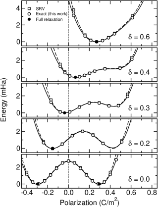
Figure 2: Energy versus polarization along the $c$ axis for the broken-inversion-symmetry perovskite described in the text, for different values of $\delta$. The solid (dashed) line is a polynomial fit of the values obtained using our (the SRV) method.

On the other hand, the electronic response is found to be profoundly important to the dielectric behavior in the case of a III-V semiconductor like AlAs, as can be seen in Fig. 3. Here we employed ABINIT abinit using the LDA Ceperley1980PRL , a plane-wave cutoff of 9 Ha, a $6\times 6\times 6$ reciprocal space grid Monkhorst1979PRB , Troullier-Martins Troullier1991PRB pseudopotentials pseudosAlAs , and a theoretically optimized lattice constant of $a=10.62$ a.u. As can be seen in Fig. 3, there is a drastic difference between the $E$ versus $P$ curves computed using the SRV method (ionic response only) and the one found with our new method (ionic and electronic response). In order to quantify this difference, the dielectric constant in both cases was computed from the curvature at the minimum of each function as $\epsilon=1+4\pi/({d^{2}E}/{dP^{2}})$. When computed with the SRV method, $\epsilon=3.0$, while when we use our new method, $\epsilon=10.3$. The experimental result is $\epsilon=10.1$ Souza2002PRL .

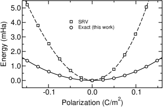
Figure 3: Energy versus magnitude of polarization in the line joining two nearest Al and As neighbors. The solid (dashed) line is a polynomial fit of the values obtained using our (the SRV) method.

Our last example involves potassium nitrate, which has an interesting phase diagram that includes a reentrant ferroelectric phase (phase III, R3m), and that has been proposed as a promising material to be used in random-access memory devices Scott1987PRB . The unit cell of phase III KNO₃ is a five-atom rhombohedral cell that results in alternating planes of K atoms and NO₃ groups arranged in such a way that the K atom is not equidistant from the NO₃ groups above and below it, but instead is slightly displaced in the vertical direction, giving rise to a polar structure. Figs. 4(a)-(b) show the conventional 15-atom hexagonal cell that is most convenient for visualization. The calculations are performed using ABINIT abinit , the LDA Ceperley1980PRL , a plane-wave cutoff of 30 Ha, a reciprocal space grid with 6 inequivalent points, and Troullier-Martins Troullier1991PRB pseudopotentials pseudosKNO3 . The theoretical structural optimization of bulk ferroelectric KNO₃ gives hexagonal lattice parameters of $a=9.68$ a.u. and $c=14.86$ a.u., to be compared with the ones found experimentally at 91 ^∘C, $a=10.37$ a.u. and $c=17.30$ a.u. Nimmo1976AC . As for the internal degrees of freedom, the distance between a K atom and the N atom above it is found to be $z=0.57c$ (experimentally, $z=0.59c$ Nimmo1976AC ), while the N–O distance is $d=2.35$ a.u. (experimentally, $d=2.42$ a.u. Nimmo1976AC ). The computation of the polarization gives 0.16 C/m², higher than the experimental values of 0.08–0.11 C/m² given in Ref. Sawada1958JPSJ, . (This disagreement is related to the reduction in volume found theoretically; when we performed an optimization of the atomic positions using the experimental lattice constants, we found a polarization value of 0.075 C/m².)

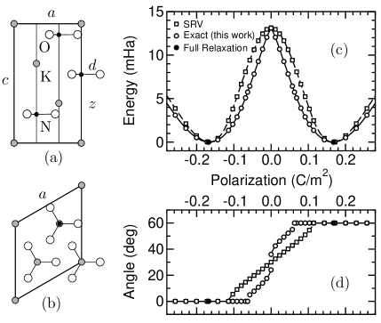
Figure 4: (a) Side view of the ferroelectric phase of KNO₃ (phase III), with the $c$ hexagonal lattice axis running vertically. (b) Top view of the same structure. (c) Energy versus polarization ${\bf P}=(0,0,P)$. (d) Angle of rotation of the NO₃ group as a function of polarization $P$.

Fig. 4(c) shows the energy of the ferroelectric phase of KNO₃ as a function of the magnitude of the polarization along the $c$ axis. As in the case of perovskites, we can see a double well potential, but now the change of polarization given by the movement of the NO₃ atoms parallel to the $c$ axis is accompanied by a rotation of these groups in their plane, as shown in Fig. 4(d). When doing SRV calculations, both the derivative of the energy and the angle of rotation are continuous functions of the polarization, and the NO₃ group rotates from $0^{\circ}$ to $60^{\circ}$ as the polarization goes from negative to positive, with the paraelectric configuration that corresponds to the maximum of $E(P)$ being the highly symmetrical one in which $z=0.5$ and the rotation angle is $30^{\circ}$. However, when the new exact method is used, this behavior changes noticeably: the $E(P)$ curve has a discontinuous derivative at $P=0$, and the angle-rotation curve is no longer continuous.

Although it may seem puzzling that the response of the system changes so significantly just by including the electronic response, this behavior can be understood on the basis of a simple model in which the energy is a function not only of polarization $P$, but also of the rotation angle $\theta$. To understand the qualitative features, it is sufficient to consider a low-order expansion $E(P,\theta)=\cos 6\theta+\alpha\cos 12\theta+\beta P\cos 3\theta+P^{2}$. We assume that $\beta>2\sqrt{2}$, in which case $E(P)$ has two minima. Then, depending on the value of $\alpha$, the behavior can be continuous ($\alpha<1/4$) or discontinuous ($\alpha>1/4)$ in $P$. Here, it appears that the system was already close to this critical value of $\alpha$, and inclusion of electronic effects happened to shift the system from the continuous to the discontinuous regime. A more detailed discussion of this material, and its modeling along the lines sketched above, will be given elsewhere. In any case, the ability of our approach to describe the complexity of the structural behavior of KNO₃ under polarization reversal provides an excellent example of the power of the method.

To summarize, we have presented a method for finding the most stable structural configuration of an insulating crystal when its electric polarization is constrained to take on a given value. Our method builds upon an earlier approach Sai2002PRB that makes the approximation of including only the lattice response to applied electric fields. By using the recently-developed theory of finite electric fields Souza2002PRL to include also the electronic response of the system, we have developed a new approach that is, instead, exact. We have illustrated the method by obtaining $E(P)$ curves for three rather different kinds of insulating materials, and have illustrated how the method is capable of describing the complexity of the nonlinear structural and dielectric response.

- (1) R. D. King-Smith and D. Vanderbilt, Phys. Rev. B 47, R1651 (1993).
- (2) I. Souza, J. Íñiguez, and D. Vanderbilt, Phys. Rev. Lett. 89, 117602 (2004).
- (3) S. de Gironcoli, S. Baroni, and R. Resta, Phys. Rev. Lett. 62, 2853 (1989); P. Giannozzi, S. de Gironcoli, P. Pavone, and S. Baroni, Phys. Rev. B 43, 7231 (1991); X. Gonze, Phys. Rev. B 55, 10337 (1997).
- (4) N. Sai, K. M. Rabe, and D. Vanderbilt, Phys. Rev. B 66, 104108 (2002).
- (5) H. Fu and L. Bellaiche, Phys. Rev. Lett. 91, 057601 (2003).
- (6) X. Wu, O. Diéguez, K. M. Rabe, and D. Vanderbilt, in preparation.
- (7) The ABINIT code is a common project of the Université Catholique de Louvain, Corning Incorporated, and other contributors (www.abinit.org). See: X. Gonze and others, Comp. Mat. Science 25, 478 (2002).
- (8) P. Hohenberg and W. Kohn, Phys. Rev. 136, B864 (1964).
- (9) D. M. Ceperley and B. J. Alder, Phys. Rev. Lett. 45, 566 (1980).
- (10) W. Kohn and L. J. Sham, Phys. Rev. 140, A1133 (1965).
- (11) H. J. Monkhorst and J. D. Pack, Phys. Rev. B 13, 5188 (1976).
- (12) N. Troullier and J. L. Martins, Phys. Rev. B 43, 1993 (1991).
- (13) More details about the pseudopotentials can be found in Ref. Sai2002PRB, .
- (14) The actual pseudopotentials files used are available at www.abinit.org/Psps/?text=../Psps/LDA_TM/lda.
- (15) J. F. Scott, M. S. Zhang, R. B. Godfrey, C. Araujo, and L. McMillan, Phys. Rev. B 35, 4044 (1987).
- (16) The actual pseudopotentials files used are available at www.abinit.org/Psps/?text=../Psps/LDA_FHI/fhi.
- (17) J. K. Nimmo and B. W. Lucas, Acta Cryst. B 32, 1968 (1976).
- (18) S. Sawada, S. Nomura, and Y. Asao, J. Phys. Soc. Jpn. 13, 1549 (1958).