Adiabatic-Impulse approximation for avoided level crossings: from phase transition dynamics to Landau-Zener evolutions and back again

Abstract

We show that a simple approximation based on concepts underlying the Kibble-Zurek theory of second order phase transition dynamics can be used to treat avoided level crossing problems. The approach discussed in this paper provides an intuitive insight into quantum dynamics of two level systems, and may serve as a link between the theory of dynamics of classical and quantum phase transitions. To illustrate these ideas we analyze dynamics of a paramagnet-ferromagnet quantum phase transition in the Ising model. We also present exact unpublished solutions of the Landau-Zener like problems.

I Introduction

Two level quantum systems that undergo avoided level crossing play an important role in physics. Often they provide not only a qualitative description of system properties but also a quantitative one. The possibility for a successful two level approximation arises in different physical systems, e.g., a single one-half spin; an atom placed in a resonant light; smallest quantum magnets; etc.

In this paper we focus on avoided level crossing dynamics in two level quantum systems. Two interesting related extensions of above mentioned long list are the critical dynamics of quantum phase transitions subir ; dorner ; jacek ; polkovnikov ; ralf and adiabatic quantum computing ad_q_com . In both of these cases (and, indeed, in all of the other applications of the avoided level crossing scenario) there are many more than two levels, but the essence of the problem can be still captured by the two level, Landau-Zener type, calculation.

Our interest in Landau-Zener model originates also from its well known numerous applications to different physical systems. In many cases there is a possibility of more general dependence of the relevant parameters (i.e. gap between the two levels on time) than in the original Landau-Zener treatment. This motivates our extensions in this paper of the level crossing dynamics to asymmetric level crossings and various power-law dependences. Appropriate variations of external parameters driving Landau-Zener transition can allow for an experimental realization of these generalized Landau-Zener like models in quantum magnets magnet and optical lattices bloch .

We focus on evolutions that include both adiabatic and diabatic (impulse) regime during a single sweep of a system parameter. For simplicity, we call these evolutions diabatic since we assume that they include a period of fast change of a system parameter. This is in contrast to adiabatic time evolutions induced by very slow parameter changes when the system never leaves adiabatic regime. We will use a formalism proposed recently by one of us bodzio . It originates from the so-called Kibble-Zurek (KZ) theory of topological defect production in the course of classical phase transitions kibble ; zurek , and works best for two level systems. The two level approximation was recently shown by Zurek et al dorner and Dziarmaga jacek to be useful in studies of quantum phase transitions confirming earlier expectations – see Chap. 1.1 of subir and bodzio . Therefore, we expect that the formalism presented here will provide a link between dynamical studies of classical and quantum phase transitions.

The present contribution extends the ideas presented in bodzio . In particular, we have succeeded in replacing the fit to numerics used there for getting a free parameter of the theory, with a simple analytic calculation. We also show that the method of bodzio can be successfully applied to a large class of two level systems. Moreover, we present nontrivial exact analytic solutions for Landau-Zener model and the relevant adiabatic-impulse approximations not published to date.

Section II presents basics of what we call the adiabatic-impulse approximation. Section III shows adiabatic-impulse, diabatic and finally exact solutions to different versions of the Landau-Zener problem. In Section IV we discuss solutions for a whole class of two level systems on the basis of adiabatic-impulse and diabatic schemes. Section V presents how results of Section III can be used to study quantum Ising model dynamics. Details of analytic calculations are in Appendix A (diabatic solutions), Appendix B (exact solutions of Landau-Zener problems) and Appendix C (adiabatic-impulse solution from Sec. IV).

II Adiabatic-Impulse approximation

We will study dynamics of quantum systems by assuming that it includes adiabatic (no population transfer between instantaneous energy eigenstates), and impulse (no changes in the wave function except for an overall phase factor) stages only. The nature of this approach suggests the name adiabatic-impulse (AI) approximation. The AI approach originates from the Kibble-Zurek (KZ) theory of nonequilibrium classical phase transitions and we refer the reader to bodzio for a detailed discussion of AI-KZ connections. Below, we summarize basic ideas of the KZ theory, and the relevant assumptions used later on.

Second order phase transitions and avoided level crossings share one key distinguishing characteristic: in both cases sufficiently near the critical point (defined by the relaxation time or by the inverse of the size of the gap between the two levels) system “reflexes” become very bad. In phase transitions this is known as “critical slowing down”.

In the treatment of the second order phase transitions this leads to the behavior where the state of the system can initially – in the adiabatic region far away from the transition – adjust to the change of the relevant parameter that induces the transition, but sufficiently close to the critical point its reflexes become too slow for it to react at all. As a consequence, a sequence of three regimes (adiabatic, impulse near the critical point, and adiabatic again on the other side of the transition) can be anticipated. In the second order phase transitions this allows one to employ a configuration dominated by the pre-transition fluctuations to calculate salient features of the post-transition state of the order parameter (e.g., the density of topological defects). Key predictions of this KZ mechanism have been by now verified in numerical simulations antunes ; laguna and more importantly in the laboratory experiments kz1 ; kz2 ; kz3 ; kz4 .

The crux of this story is of course the moments when the transition from adiabatic to impulse and back to adiabatic behavior takes place. Assuming that the transition point is crossed at time $t=0$, this must happen around the instants $\pm\hat{t}$, where $\hat{t}$ equals system relaxation time $\tau$ zurek . As the relaxation time depends on system parameter $\varepsilon$, which is changed as a function of time, one can write

$$\tau(\varepsilon(\hat{t}\,))=\hat{t}.$$ (1)

This basic equation proposed in zurek can be solved when dependence of $\tau$ on some measure of the distance from the critical point (e.g., relative temperature or coupling $\varepsilon$) is known. Assuming, e.g., $\tau=\tau_{0}/\varepsilon$ and $\varepsilon=t/\tau_{Q}$, where $\tau_{Q}$, the “quench time”, contains information about how fast the system is driven through the transition, one arrives at $\tau_{0}/(\hat{t}/\tau_{Q})=\hat{t}$. Hence, the time $\hat{t}$ at which the behavior switches between approximately adiabatic and approximately impulse is $\sqrt{\tau_{0}\tau_{Q}}$. Once this last “adiabatic” instant in the evolution of the system is known, interesting features of the post transition state (such as the size of the regions $\hat{\xi}$ in which the order parameter is smooth) can be computed. Generalization to other universality classes is straightforward zurek and leads to

$$\hat{t}\sim\tau_{Q}^{1/(1+\nu z)}\ \ \ ,\ \ \ \hat{\xi}\sim\tau_{Q}^{\nu/(1+\nu z)},$$ (2)

where $z$ and $\nu$ are universal critical exponents (see, e.g., antunes ).

In what follows we adopt this approach to quantum systems where dynamics can be approximated as an avoided level crossing (see Fig. 1). For simplicity we restrict ourselves to two-level systems that possess a single anti-crossing (Fig. 1) in the excitation spectrum and a gap preferably going to $+\infty$ far away from the anti-crossing. The latter condition guarantees that asymptotically the system enters adiabatic regime.

The passage through avoided level crossing can be divided into an adiabatic and an impulse regime according to the size of the gap in comparison with the energy scale that characterizes the rate of the imposed changes in system Hamiltonian. If the gap is large enough the system is in adiabatic regime, while when the gap is small it undergoes impulse time evolution as depicted in Fig. 1(b). The instants $\pm\hat{t}$ are supposed to be such that the discrepancy between time dependent exact results and those coming from splitting of the evolution into only adiabatic and impulse parts is minimized. Therefore, the AI approximation looks like a time dependent variational method where $\hat{t}$ is a variational parameter while adiabatic-impulse assumptions provide a form of a variational wave function.

To make sure that assumptions behind the AI approach are correctly understood, let’s consider time evolution of the system depicted in Fig. 1. Let the evolution start at $t_{i}\to-\infty$ from a ground state (GS) and last till $t_{f}\to+\infty$. The AI method assumes that the system wave function, $|\Psi(t)\rangle$, satisfies the following three approximations coming from passing through first adiabatic, then impulse and finally adiabatic regions

$$t\in[-\infty,-\hat{t}\,] : |\Psi(t)\rangle\approx({\rm phase\ factor})|{\rm GS\ at\ t}\rangle$$

$$t\in[-\hat{t},\hat{t}\,] : |\Psi(t)\rangle\approx({\rm phase\ factor})|{\rm GS\ at\ -\hat{t}}\rangle$$

$$t\in[\hat{t},+\infty] : |\langle\Psi(t)|{\rm GS\ at\ t}\rangle|^{2}={\rm const}.$$

Figure 1: Plot (a): structure of energy spectrum (parametrized by time) of a generic two-level system under consideration. Note the anticrossing at $t=0$ and asymptotic form of eigenstates: $|1\rangle$, $|2\rangle$. Plot (b): adiabatic-impulse regimes in system dynamics. Compare it to a plot of relaxation time scale in the Kibble-Zurek theory zurek ; bodzio . Note that instants separating adiabatic and impulse regimes does not have to be placed symmetrically with respect to $t=0$ – see Sec. III.1 and Fig. 3.

Finally, one needs to know how to get the instant $\hat{t}$. As proposed in bodzio , the proper generalization of Eq. (1) to the quantum case (after rescaling everything to dimensionless quantities) reads

$$\frac{1}{{\rm gap}(\hat{t}\,)}=\alpha\hat{t},$$ (3)

where $\alpha={\cal O}(1)$ is a constant. Similarity between Eq. (3) and Eq. (1) suggests (in accord with physical intuition) that the quantum mechanical equivalent of the relaxation time scale is an inverse of the gap.

In this paper we give a simple and systematic way for (i) obtaining $\alpha$ analytically; (ii) verification that Eq. (3) leads to correct results in the lowest nontrivial order. This method, illustrated on specific examples in Appendix A, is based on the observation that a time dependent Schrödinger equation can be solved exactly in the diabatic limit if one looks at the lowest nontrivial terms in expressions for excitation amplitudes. This should be true even when getting an exact solution turns out to be very complicated or even impossible. After obtaining $\alpha$ this way, the whole AI approximation is complete in a sense that there are no free parameters, so its predictions can be rigorously checked by comparison to exact (either analytic or numeric) solution.

III Dynamics in the Landau-Zener model

In this section we illustrate the AI approximation by considering the Landau-Zener model. In this way we supplement and extend the results of bodzio .

The Landau-Zener model, after rescaling all the quantities to dimensionless variables, is defined by the Hamiltonian:

$$H=\frac{1}{2}\left(\begin{array}[]{cc}\frac{t}{\tau_{Q}}&1\\ 1&-\frac{t}{\tau_{Q}}\end{array}\right),$$ (4)

where $\tau_{Q}$ is time independent and provides a time scale on which the system stays in the neighborhood of an anti-crossing. As $\tau_{Q}\to 0$ the system undergoes diabatic time evolution, while $\tau_{Q}\gg 1$ means adiabatic evolution. There are two eigenstates of this model for any fixed time $t$: the ground state $|\downarrow(t)\rangle$ and the excited state $|\uparrow(t)\rangle$ given by:

$$\left[\begin{array}[]{c}|\uparrow(t)\rangle\\ |\downarrow(t)\rangle\end{array}\right]=\left(\begin{array}[]{rr}\cos(\theta(t)/2)&\sin(\theta(t)/2)\\ -\sin(\theta(t)/2)&\cos(\theta(t)/2)\end{array}\right)\left[\begin{array}[]{c}|1\rangle\\ |2\rangle\end{array}\right],$$ (5)

where $|1\rangle$ and $|2\rangle$ are time-independent basis states of the Hamiltonian (4); $\cos(\theta)=\varepsilon/\sqrt{1+\varepsilon^{2}}$; $\sin(\theta)=1/\sqrt{1+\varepsilon^{2}}$;

$$\varepsilon=\frac{t}{\tau_{Q}},$$ (6)

and $\theta\in[0,\pi]$. The gap in this model is

$${\rm gap}=\sqrt{1+\varepsilon^{2}}.$$

The instant $\hat{t}$ is obtained from Equation (3):

$$\frac{1}{\sqrt{1+\left(\frac{\hat{t}}{\tau_{Q}}\right)^{2}}}=\alpha\hat{t},$$

which leads to the following solution

$$\hat{\varepsilon}=\frac{\hat{t}}{\tau_{Q}}=\frac{1}{\sqrt{2}}\sqrt{\sqrt{1+\frac{4}{(\alpha\tau_{Q})^{2}}}-1}.$$ (7)

Dynamics of the system is governed by the Schrödinger equation:

$$i\frac{d}{dt}|\Psi\rangle=H|\Psi\rangle,$$

and it will be assumed that evolution happens in the interval $[t_{i},t_{f}]$.

As was discussed in bodzio , by using AI approximation one can easily arrive at the following predictions for the probability of finding the system in the excited state at $t_{f}\gg\hat{t}$

• time evolution starts at $t_{i}\ll-\hat{t}$ from the ground state

  $$P_{AI}=|\langle\uparrow(\hat{t}\,)|\downarrow(-\hat{t}\,)\rangle|^{2}=\frac{\hat{\varepsilon}^{2}}{1+\hat{\varepsilon}^{2}}.$$ (8)

  In this case the system undergoes in the AI scheme the adiabatic time evolution from $t_{i}$ to $-\hat{t}$, then impulse one from $-\hat{t}$ to $\hat{t}$ and finally adiabatic from $\hat{t}$ to $t_{f}\gg\hat{t}$.

• time evolution starts at $t_{i}=0$ from the ground state

  $$p_{AI}=|\langle\uparrow(\hat{t}\,)|\downarrow(0)\rangle|^{2}=\frac{1}{2}\left(1-\frac{1}{\sqrt{1+\hat{\varepsilon}^{2}}}\right).$$ (9)

  Now evolution is first impulse from $t=0$ to $t=\hat{t}$ and then adiabatic from $\hat{t}$ to $t_{f}\gg\hat{t}$.

In the following we consistently denote excitation probability when the system evolves from $t_{i}\ll-\hat{t}$, $t_{i}=0$ by $P$, $p$ respectively. Additionally the subscript AI will be attached to predictions based on the AI approximation.

In the first case, the substitution of (7) into (8) leads to

$$P_{AI}=1-\alpha\tau_{Q}+\frac{(\alpha\tau_{Q})^{2}}{2}-\frac{(\alpha\tau_{Q})^{3}}{8}+{\cal O}(\tau_{Q}^{4}).$$ (10)

Now we have to determine $\alpha$. It turns out that it can be done by looking at the diabatic excitation probability. The proper expression and calculation can be found in Appendix A. Substituting $\eta=1/2$ into (37) and (36) one gets that to the lowest nontrivial order $P_{AI}=1-\pi\tau_{Q}/2$, which implies that $\alpha=\pi/2$ and verifies Eq. (3) for this case. Note that the calculation leading to Eqs. (36) and (37) is not only much easier then determination of exact LZ solution zener , but also really elementary. Therefore, we expect that it can be done comparably easily for any model of interest.

Now we are ready to compare our AI approximation with $\alpha$ determined as above, to the exact result, i.e.,

$$P=\exp\left(-\frac{\pi\tau_{Q}}{2}\right).$$ (11)

First, the agreement between the exact and AI result is up to ${\cal O}(\tau_{Q}^{3})$, i.e., one order above the first nontrivial term. This is the advantage that the AI approximation provides over a simple diabatic approximation performed in Appendix A. Second, we see that the AI expansion contains the same powers of $\tau_{Q}$ as the diabatic (small $\tau_{Q}$) expansion of the exact result. Third, Fig. 2 quantifies the discrepancies between exact, AI and diabtic results. For the AI prediction, we plot in Fig. 2 instead of a Taylor series (10) the full expression evaluated in bodzio

$$P_{AI}=\frac{2}{(\alpha\tau_{Q})^{2}+\alpha\tau_{Q}\sqrt{(\alpha\tau_{Q})^{2}+4}+2},$$ (12)

with $\alpha=\pi/2$. As easily seen the AI approximation significantly outperforms a diabatic solution. In other words, the combination of AI simplification of dynamics and diabatic prediction for the purpose of getting the constant $\alpha$ leads to fully satisfactory results considering simplicity of the whole approach.

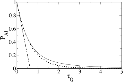
Figure 2: Transition probability when the system starts time evolution from a ground state at $t_{i}\to-\infty$ and evolves to $t_{f}\to+\infty$. Dots: exact expression (11). Solid line: AI prediction (12) with $\alpha=\pi/2$ determined from diabatic solution in Appendix A. Dashed thick line: lowest order diabatic result, $1-\pi\tau_{Q}/2$, coming from (36) and (37) with $\eta=1/2$.

It is instructive to consider now separately three situations: (i) dynamics in a nonsymmetric avoided level crossing (Sec. III.1); (ii) dynamics beginning at the anti-crossing center (Sec. III.2); and (iii) dynamics starting at $t_{i}\to-\infty$ but ending at the anti-crossing center (Sec. III.3). The first case will give us a hint whether ${\cal O}(\tau_{Q}^{3})$ agreement we have seen above is accidental and has something to do with the symmetry of the Landau-Zener problem. The second problem was preliminarily considered in bodzio , but without comparing the AI prediction to exact analytic one being interesting on its own. Finally, the third problem is an example where AI approximation correctly suggests at a first sight unexpected symmetry between this problem and the one considered in Sec. III.2.

III.1 Nonsymmetric Landau-Zener problem

Figure 3: The same as in Fig. 1 but for nonsymmetric Landau-Zener problem with $\delta>1$ – see (13).

We assume that system Hamiltonian is provided by the following expression

$$H=\frac{1}{2}\left(\begin{array}[]{cc}\frac{1}{\chi}\frac{t}{\tau_{Q}}&1\\ 1&-\frac{1}{\chi}\frac{t}{\tau_{Q}}\end{array}\right)\ \ \ ,\ \ \ \chi=\left\{\begin{array}[]{c}1\ {\rm for}\ t\leq 0\\ \delta\ {\rm for}\ t>0\\ \end{array}\right.$$ (13)

with $\delta>0$ being the asymmetry parameter – see Fig. 3(a) for schematic plot of the spectrum.

Once again, evolution starts at $t_{i}\to-\infty$ from a ground state. The exact expression for finding the system in the excited eigenstate at the end of time evolution ($t_{f}\to+\infty)$ is

$$P = 1-\frac{e^{-\frac{1}{8}\pi(1+\delta)\tau_{Q}}}{2}\sinh\left(\frac{1}{4}\pi\tau_{Q}\delta\right)$$ (14)

$$\left|\frac{\Gamma(1/2+i\tau_{Q}\delta/8)}{\Gamma(1/2+i\tau_{Q}/8)}+\sqrt{\frac{1}{\delta}}\frac{\Gamma(1+i\tau_{Q}\delta/8)}{\Gamma(1+i\tau_{Q}/8)}\right|^{2},$$

and its derivation is presented in Appendix B. Naturally, for $\delta=1$, i.e., in a symmetric LZ problem, the expression (14) reduces to (11).

Now we would like to compare (14) to predictions coming from AI approximation. Due to asymmetry of the Hamiltonian the systems enters the impulse regime in the time interval $[-\hat{t}_{L},\hat{t}_{R}]$ – see Fig. 3(b) for illustration of these concepts. The instants $\hat{t}_{L}$ and $\hat{t}_{R}$ are easily found in the same way as in the symmetric case. It is a straightforward exercise to verify that according to AI approximation, the probability of finding the system in the upper state is

$$P_{AI}=|\langle\downarrow(-\hat{t}_{L})|\uparrow(\hat{t}_{R})\rangle|^{2}.$$ (15)

To simplify comparison between exact (14) and approximate (15) excitation probabilities we will present their diabatic Taylor expansions:

$$P_{AI} = 1-\frac{1}{4}\left(1+\sqrt{\delta}\right)^{2}\alpha\tau_{Q}+$$ (16)

$$\frac{1}{16}(1+\delta)(1+\sqrt{\delta})^{2}(\alpha\tau_{Q})^{2}+{\cal O}(\tau_{Q}^{3}).$$

Determination of the constant $\alpha$ is easy and is presented in Appendix A. By putting $\eta=1/2$ into (37) and (41), one gets that $\alpha=\pi/2$.

The AI prediction can be easily compared to the exact result (14) after series expansion

$$P=1-\frac{\pi}{8}\left(1+\sqrt{\delta}\right)^{2}\tau_{Q}+\frac{\pi^{2}}{64}(1+\delta)(1+\sqrt{\delta})^{2}\tau_{Q}^{2}+{\cal O}(\tau_{Q}^{3}).$$

This comparison shows that once again there is perfect matching between exact and AI description up to ${\cal O}(\tau_{Q}^{3})$, i.e., one order better then the simple diabatic approximation from Appendix A, despite the fact that we deal now with nonsymmetric LZ problem. Moreover, the constant $\alpha$ is the same in symmetric and nonsymmetric cases. Finally the same powers of $\tau_{Q}$ show up in both exact and AI results.

The nonsymmetric Landau-Zener model is also interesting in the light of a recent paper ray , where it is argued that the final state of the system that passed through a classical phase transition point, is determined by details of dynamics after phase transition. In our system, there are two different quench rates: $\tau_{Q}$ before the transition and $\tau_{Q}^{\prime}=\tau_{Q}\delta$ after the transition. Substitution of $\delta=\tau_{Q}^{\prime}/\tau_{Q}$ into (14) shows that the final state of nonsymmetric Landau-Zener model expressed in terms of the excitation probability depends on both $\tau_{Q}$ and $\tau_{Q}^{\prime}$, so that it behaves differently than the system described in ray .

III.2 Landau-Zener problem when time evolution starts at the anti-crossing center

Now we consider the LZ problem characterized by Hamiltonian (4) in the case when time evolution starts from the ground state at the anticrossing center, i.e., $t_{i}=0$. It means that $|\Psi(0)\rangle\propto\left(|1\rangle-|2\rangle\right)/\sqrt{2}$. Excitation probability at $t_{f}\to+\infty$ equals exactly (see Appendix B)

$$p = 1-\frac{2}{\pi\tau_{Q}}\sinh\left(\frac{\pi\tau_{Q}}{4}\right)e^{-\pi\tau_{Q}/8}\left|\Gamma\left(1+\frac{i\tau_{Q}}{8}\right)+\right.$$ (17)

$$\left.e^{i\pi/4}\sqrt{\frac{\tau_{Q}}{8}}\Gamma\left(\frac{1}{2}+\frac{i\tau_{Q}}{8}\right)\right|^{2}.$$

From the point of view of AI approximation the evolution is now simplified by assuming that it is impulse from $t_{i}=0$ to $\hat{t}$ and then adiabatic from $\hat{t}$ to $t_{f}\to+\infty$. This case was discussed in bodzio , and it was shown that substitution of (7) into (9) leads to a simple expression

$$p_{AI}=\frac{1}{2}-\frac{1}{2}\sqrt{1-\frac{2}{(\alpha\tau_{Q})^{2}+\alpha\tau_{Q}\sqrt{(\alpha\tau_{Q})^{2}+4}+2}},$$ (18)

expanding it into diabatic series one gets

$$p_{AI}=\frac{1}{2}-\frac{1}{2}\sqrt{\alpha\tau_{Q}}+\frac{1}{8}(\alpha\tau_{Q})^{3/2}+{\cal O}(\tau_{Q}^{5/2}).$$ (19)

Determination of a constant $\alpha$ is straightforward (see Appendix A). Putting $\eta=1/2$ into (39,40) one easily gets $\alpha=\pi/4$ and confirms that the first nontrivial term in (19) is indeed $\propto\sqrt{\tau_{Q}}$. This value of $\alpha$ ($\approx 0.785$) is in agreement with the numerical fit done in bodzio where optimal $\alpha$ was found to be equal to $0.77$. Small disagreement comes from the fact that now we use just the $\frac{1}{2}-\frac{1}{2}\sqrt{\alpha\tau_{Q}}$ part for getting $\alpha$, which is equivalent to making the fit to exact results in the limit of $\tau_{Q}\ll 1$. In bodzio the fit of the whole expression (18) in the range of $0<\tau_{Q}<6$ was done.

Having the exact solution (17) at hand, we can verify rigorously accuracy of (18,19) with the choice of $\alpha=\pi/4$. Expanding (17) into diabatic series one gets

$$p=\frac{1}{2}-\frac{\sqrt{\pi}}{4}\sqrt{\tau_{Q}}+\frac{\pi^{3/2}}{64}\left(2-\frac{4\ln 2}{\pi}\right)\tau_{Q}^{3/2}+{\cal O}(\tau_{Q}^{5/2}).$$ (20)

As expected the first nontrivial term is in perfect agreement with (19) once $\alpha=\pi/4$. On the other hand, the term proportional to $\tau_{Q}^{3/2}$ is about $10\%$ off. Indeed, after substitution $\alpha=\pi/4$ into (19) one gets the third term equal to $\pi^{3/2}\tau_{Q}^{3/2}/64$, which has to be compared to $\approx 1.1\pi^{3/2}\tau_{Q}^{3/2}/64$ from (20). It shows that the AI approximation in this case does not predict exactly higher nontrivial terms in the diabatic expansion.

Nonetheless, expression (18) works much better then the above comparison suggests. It not only significantly outperforms the lowest order diabatic expansion, $\frac{1}{2}-\frac{1}{4}\sqrt{\pi\tau_{Q}}$, but also beautifully fits to the exact result pretty far from the $\tau_{Q}\ll 1$ regime. Fig. 4 leaves no doubt about these statements. It suggests that AI predictions should be compared to exact results not only term by term as in the diabatic expansion, but also in a full form.

Figure 4: Transition probability when the system starts time evolution at the anti-crossing center from a ground state and evolves to $t_{f}\to+\infty$. Dots: exact expression (17). Solid line: AI prediction (18) with $\alpha=\pi/4$ determined from the diabatic solution in Appendix A. Dashed thick line: lowest order diabatic prediction $1/2-\sqrt{\pi\tau_{Q}}/4$ coming from (39,40) with $\eta=1/2$.

III.3 One half of Landau-Zener evolution

In this section we consider exactly one half of the LZ problem. Namely, we take the Hamiltonian (4) and evolve the system to the anti-crossing center, $t_{f}=0$, while starting from the ground state at $t_{i}\to-\infty$.

Let’s see what the AI approximation predicts for excitation probability of the system at $t_{f}=0$. According to AI, evolution is adiabatic in the interval $[-\infty,-\hat{t}\,]$ and then impulse in time range $[-\hat{t},0]$. It implies that

$$|\langle\uparrow(0)|\Psi(0)\rangle|^{2}\approx|\langle\uparrow(0)|\Psi(-\hat{t}\,)\rangle|^{2}\approx|\langle\uparrow(0)|\downarrow(-\hat{t}\,)\rangle|^{2}.$$

A simple calculation then shows that

$$P_{AI}=|\langle\uparrow(0)|\downarrow(-\hat{t}\,)\rangle|^{2}=\frac{1}{2}\left(1-\frac{1}{\sqrt{1+\hat{\varepsilon}^{2}}}\right).$$ (21)

A quick look at (9) shows that the excitation probability for one-half of the Landau-Zener problem is supposed to be, according to the AI scheme, equal to the excitation probability when the system starts from the anti-crossing and evolves toward $t_{f}\to+\infty$.

To check that prediction we have solved the one-half LZ model exactly, see Appendix B, and found that indeed both probabilities are exactly the same, so the AI approximation provides us here with a prediction that is correct not only qualitatively but also quantitatively.

IV Dynamics in a general class of quantum two level systems

To test predictions coming from the AI approximation on two level systems different than the classic Landau-Zener model, we consider in this section dynamics induced by the Hamiltonian

$$H=\frac{1}{2}\left(\begin{array}[]{cc}{\rm sgn}(t)\left|\frac{t}{\tau_{Q}}\right|^{\frac{\eta}{1-\eta}}&1\\ 1&-{\rm sgn}(t)\left|\frac{t}{\tau_{Q}}\right|^{\frac{\eta}{1-\eta}}\end{array}\right),$$ (22)

where $\eta\in(0,1)$ is a constant parameter (when $\eta=1/2$ the system reduces to the Landau-Zener model). The eigenstates of Hamiltonian (22) are expressed by formula (5) with

$$\cos(\theta)=\frac{{\rm sgn}(t)\left|\frac{t}{\tau_{Q}}\right|^{\frac{\eta}{1-\eta}}}{\sqrt{1+\left|\frac{t}{\tau_{Q}}\right|^{\frac{2\eta}{1-\eta}}}},$$

and

$$\sin(\theta)=\frac{1}{\sqrt{1+\left|\frac{t}{\tau_{Q}}\right|^{\frac{2\eta}{1-\eta}}}}.$$

Extending the notation of Sec. III to the system (22) one has to replace definition (6) by

$$\varepsilon={\rm sgn}(t)\left|\frac{t}{\tau_{Q}}\right|^{\frac{\eta}{1-\eta}}$$

and then expressions (8,9) providing excitation probabilities are valid also for the model (22).

The instant $\hat{t}$ for the Hamiltonian (22) is determined by the following version of Eq. (3)

$$\frac{1}{\sqrt{1+\left|\frac{\hat{t}}{\tau_{Q}}\right|^{\frac{2\eta}{1-\eta}}}}=\alpha\hat{t}.$$ (23)

It seems to be impossible to obtain solution of (23) exactly. Fortunately, a diabatic perturbative expansion for $\hat{t}$ can be found – see Appendix C. Once the diabatic expansion of $\hat{t}$ is known, we can present different predictions about dynamics of the model (22).

First, we consider transitions starting from a ground state at $t_{i}\to-\infty$ and lasting till $t_{f}\to+\infty$. Using the results of Appendix C one gets the following expression for the excitation probability:

$$P_{AI} = \frac{\hat{\varepsilon}^{2}}{1+\hat{\varepsilon}^{2}}=1-(\alpha\tau_{Q})^{2\eta}+(1-\eta)(\alpha\tau_{Q})^{4\eta}-$$ (24)

$$\frac{1}{2}(1-\eta)(2-3\eta)(\alpha\tau_{Q})^{6\eta}+\frac{1}{3}(1-\eta)(1-2\eta)$$

$$(3-4\eta)(\alpha\tau_{Q})^{8\eta}+{\cal O}\left(\tau_{Q}^{10\eta}\right).$$

This result is equivalent to (10) when one puts $\eta=1/2$. The constant $\alpha$ was found in Appendix A from the diabatic solution and equals (37)

$$\alpha=(1-\eta)\Gamma(1-\eta)^{\frac{1}{\eta}}.$$

The exponent $2\eta$ in the lowest order term in (24) was positively verified (Appendix A). Additionally, we have performed numerical simulations for $\eta=1/3,2/3,3/4,5/6$. A fit to numerics in the range of $\tau_{Q}\ll 1$ has confirmed both the exponent $2\eta$ and the value of $\alpha$. The comparison between the AI prediction for $\eta=1/3,2/3$ and numerics is presented in Fig. 5(a). The lack of exact solution for this problem does not allow us for a more systematic analytic investigation of the AI approximation in this case. Nonetheless, a good agreement between AI and numerics is easily noticed. Once again, the AI prediction outperforms the lowest order diabatic expansion.

As before, we would like to consider transitions starting from the anticrossing center, i.e., $t_{i}=0$. In this case the excitation probability equals

$$p_{AI} = \frac{1}{2}\left(1-\frac{1}{\sqrt{1+\hat{\varepsilon}^{2}}}\right)=\frac{1}{2}-\frac{1}{2}(\alpha\tau_{Q})^{\eta}+\frac{1}{4}(1-\eta)$$ (25)

$$(\alpha\tau)^{3\eta}-\frac{1}{16}(1-\eta)(3-5\eta)(\alpha\tau_{Q})^{5\eta}+$$

$${\cal O}\left(\tau_{Q}^{7\eta}\right),$$

As above, the diabatic calculation of Appendix A verifies the exponent of the first nontrivial term in (25) and provides us with the following prediction for $\alpha$ (40)

$$\alpha=(1-\eta)\Gamma(1-\eta)^{\frac{1}{\eta}}\cos\left(\frac{\pi}{2}\eta\right)^{\frac{1}{\eta}}.$$

After setting $\eta=1/2$ formula (25) becomes the same as (19). Due to the lack of exact results we have carried out numerical simulations for $\eta=1/3,2/3,3/4,5/6$. As expected, this calculation has confirmed that the exponent of $\tau_{Q}$ is indeed $\eta$ for small $\tau_{Q}$ and that $\alpha$ is provided by (40). The AI approximation vs. numerics and diabatic expansion for $\eta=1/3,2/3$ is presented in Fig. 5(b). Once again an overall agreement is strikingly good.

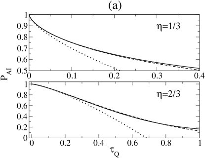
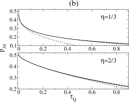
Figure 5: Numerics: bold dashed line, AI approximation: solid line, lowest order exact diabatic expansion (Appendix A): dotted line. (a): evolution starts from $t_{i}\to-\infty$. (b): evolution starts from $t_{i}=0$. In both (a) and (b) plots evolution ends in $t_{f}\to+\infty$.

V Quantum phase transition in Ising model vs. adiabatic-impulse approach

In this section we will illustrate how ideas coming from the adiabatic-impulse approach can be used in studies of dynamics of quantum phase transition. As an example we choose the quantum Ising model recently considered in this context dorner ; jacek ; polkovnikov . The quantum Ising model is defined by the following Hamiltonian:

$$H=-\sum_{n=1}^{N}\left(g\sigma^{x}_{n}+\sigma^{z}_{n}\sigma^{z}_{n+1}\right),$$ (26)

where $N$ is the number of spins. The quantum phase transition in this model is driven by the change of a dimensionless coupling $g$. The transition point between paramagnetic phase ($g>1$) and ferromagnetic one ($0\leq g<1$) is at $g=1$. To study dynamics of (26) one assumes that the system evolves from time $t^{\prime}=-\infty$ to time $t^{\prime}=0$, and takes

$$g=-\frac{t^{\prime}}{\tau_{Q}^{\prime}},$$

where $\tau_{Q}^{\prime}$ provides a quench rate. The quantity of interest is density of topological defects (kinks) after completion of the transition, i.e., at $g=0$. It equals jacek

$$n=\lim_{N\to+\infty}\left\langle\frac{1}{2N}\sum_{n=1}^{N-1}(1-\sigma^{z}_{n}\sigma^{z}_{n+1})\right\rangle.$$ (27)

The quantum Ising model obviously possesses $2^{N}$ different energy eigenstates so it seems to be hopeless to expect that the two level approximation would be sufficient. Therefore, it is a remarkable result of Dziarmaga jacek , that dynamics in this system can be exactly described by a series of uncoupled Landau-Zener systems. Due to lack of space, we refer the reader to jacek , and present just the main results and their AI equivalents.

The density of defects (27) in Dziarmaga’s notation reads as

$$n\stackrel{{\scriptstyle N\gg 1}}{{=}}\frac{1}{2\pi}\int_{-\pi}^{\pi}{\rm d}k\,p_{k},$$

where $p_{k}$’s are defined as

$$p_{k}=|\cos(k/2)u_{k}(t^{\prime}=0)-\sin(k/2)v_{k}(t^{\prime}=0)|^{2},$$ (28)

with $u_{k}$, $v_{k}$ satisfying the following Landau-Zener system

$$\frac{d}{dt}\left(\begin{array}[]{c}v_{k}\\ u_{k}\end{array}\right)=\frac{1}{2}\left(\begin{array}[]{cc}\frac{t}{\tau_{Q}}&1\\ 1&-\frac{t}{\tau_{Q}}\end{array}\right)\left(\begin{array}[]{c}v_{k}\\ u_{k}\end{array}\right),$$ (29)

$$t=4\left(t^{\prime}+\tau_{Q}^{\prime}\cos k\right)\sin k,$$

$$\tau_{Q}=4\tau_{Q}^{\prime}\sin^{2}k,$$

where $t^{\prime}$ changes from $-\infty$ to $0$. The initial conditions for that LZ system are the following

$$|u_{k}(t^{\prime}=-\infty)|=1\ \ \ ,\ \ \ v_{k}(t^{\prime}=-\infty)=0.$$ (30)

Due to the symmetry of the whole problem, it is possible to show that $p_{k}\equiv p_{-k}$, and therefore it is sufficient to restrict to $k\geq 0$ from now on.

Evolution in (29) lasts from $t_{i}=-\infty$ to $t_{f}=2\tau_{Q}^{\prime}\sin(2k)$. Since obviously $t_{f}$ does not go to $+\infty$, it is important to determine where $t_{f}$ is placed with respect to $\pm\hat{t}$.

We solve the equation $\hat{t}=|t_{f}|$ (where we substitute $k=k_{c}$). After using (7) with $\alpha=\pi/2$, and simple algebra one arrives at

$$\frac{1}{\sqrt{2}}\sqrt{\sqrt{1+\frac{4}{(\pi\tau_{Q}/2)^{2}}}-1}=\left|\frac{\cos k_{c}}{\sin k_{c}}\right|,$$

which leads to the result

$$\sin^{2}k_{c}=1-\frac{1}{4\pi^{2}\tau_{Q}^{\prime\,2}}.$$

Defining $k_{c}$ to be between $0$ and $\pi/2$ and doing some additional easy calculations one gets that when $\tau_{Q}^{\prime}>\frac{1}{2\pi}$ we have: (i) $t_{f}\geq\hat{t}$ for $k\in[0,k_{c}]$; (ii) $-\hat{t}<t_{f}<\hat{t}$ for $k\in(k_{c},\pi-k_{c})$; (iii) $t_{f}\leq-\hat{t}$ for $k\in[\pi-k_{c},\pi]$. Moreover, when $\tau_{Q}^{\prime}<\frac{1}{2\pi}$ one can show that $|t_{f}|<\hat{t}$ for any $k$’s of interest. It means that the evolution ends in the impulse regime for small enough $\tau_{Q}^{\prime}$.

Now, as in dorner ; jacek ; polkovnikov , we consider adiabatic time evolutions of the Ising model. In our scheme it clearly corresponds to $\tau_{Q}^{\prime}\gg\frac{1}{2\pi}$. As the system undergoes slow evolution it is safe to assume that only long wavelength modes are excited, which means that $k\ll\pi/4$ are of interest. This allows to approximate $\sin k\sim k$ and $\cos k\sim 1$, which implies that (28) turns into $p_{k}\approx|u_{k}(t_{f})|^{2}$ and that

$$n\approx\frac{1}{\pi}\int_{0}^{\epsilon}{\rm d}k\,|u_{k}(t_{f})|^{2},$$

with $\epsilon\ll\pi/4$. Since $k\in[0,\epsilon]$ corresponds to the above mentioned (i) case, $t_{f}>\hat{t}$ , the AI approximation says that $|u_{f}(t_{f})|\approx|u_{f}(+\infty)|$. Initial conditions (30) mean that the system starts time evolution at $t=-\infty$ from excited state and we are interested in probability of finding it in the ground state at $t_{f}$. Elementary algebra based on AI approximation shows that this probability equals

$$|u_{k}(t_{f})|^{2}=|\langle\uparrow(-\hat{t}\,)|\downarrow(\hat{t}\,)\rangle|^{2}=|\langle\downarrow(-\hat{t}\,)|\uparrow(\hat{t}\,)\rangle|^{2}.$$

Therefore, it is provided by (8) and (12). For any fixed $\epsilon$ consistent with lowest order approximation of $\sin k$ and $\cos k$ one gets

$$n\cong 0.172\frac{1}{\sqrt{2\tau_{Q}^{\prime}}},$$ (31)

where the prefactor, was found from expansion of the integral into $1/\sqrt{\tau_{Q}^{\prime}}$ adiabatic series with $\tau_{Q}^{\prime}\to+\infty$ at fixed $\epsilon$. In the derivation of this result $\sin^{2}k$ in the expression for $\tau_{Q}$ was approximated by $k^{2}$.

First of all, the prediction (31) provides correct scaling of defect density with $\tau_{Q}^{\prime}$. The prefactor, $0.172$, has to be compared to $\frac{1}{2\pi}\approx 0.16$ (exact result from jacek and numerical estimation from dorner ) or $0.18$ (approximate result from polkovnikov ). Our prefactor matches these results remarkably closely concerning simplicity of the whole AI approximation. Slight overestimation of the prefactor in comparison to exact result comes from the fact that AI transition probability, Eq. (12), overestimates the exact result, Eq. (11), for large $\tau_{Q}$’s (Fig. 2). It is interesting, to note that in the Kibble-Zurek scheme used for description of classical phase transitions an overestimation of defect density is usually of the order of ${\cal O}(1)$ dorner ; antunes ; laguna , while here discrepancy is smaller than $10\%$.

Therefore, the AI approximation provides us with two predictions concerning dynamics of the quantum Ising model: (i) it estimates when evolution ends in the asymptotic limit; (ii) it correctly predicts scaling exponent and number of defects produced during adiabatic transitions. The part (ii) can be calculated exactly in the quantum Ising model (26). Nonetheless, in other systems undergoing quantum phase transition the two level simplification might be too difficult for exact analytic treatment, e.g., as in the system governed by (22). Then the AI analysis might be the only analytic approach working beyond the lowest order diabatic expansion. Besides that the AI approach provides us with a quite intuitive description of system dynamics, which is of interest in its own. Especially, when one looks at connections between classical and quantum phase transitions.

VI Summary

We have shown that the adiabatic-impulse approximation, based on the ideas underlying Kibble-Zurek mechanism kibble ; zurek , provides good quantitative predictions concerning diabatic dynamics of two level Landau-Zener like systems. After supplementing the splitting of the evolution into adiabatic and impulse regimes by the exact lowest order diabatic calculation, the whole approach is complete and can be in principle applied to different systems possessing anti-crossings, e.g., those lacking exact analytic solution as the model (22). We expect that the AI approach will provide the link between dynamics of classical and quantum phase transition thanks to usage of the same terminology and similar assumptions.

We also expect that different variations of the classic Landau-Zener system discussed in this paper can be experimentally realized in the setting where the sweep rate can be manipulated. Indeed, the model (22) arises once a proper nonlinear change of external system parameter is performed. The experimental access to studies of nonsymmetric Landau-Zener model can be obtained by change of the sweep rate after passing an anti-crossing center. The case of evolution starting from or ending at the anticrossing center can also be subjected to experimental investigations, e.g., in a beautiful system consisting of the smallest available quantum magnets (cold Fe₈ clusters) magnet .

We are grateful to Uwe Dorner for collaboration on nonsymmetric Landau-Zener problem, and Jacek Dziarmaga for comments and useful suggestions on the manuscript. Work supported by the U.S. Department of Energy, National Security Agency, and the ESF COSLAB program.

Appendix A Exact diabatic expressions for transition probabilities

We would like to provide lowest order exact expressions for transition probabilities in a class of two level systems described by the Hamiltonian (22).

First, we express the wave function as

$$|\Psi(t)\rangle = C_{1}(t)\exp\left(\frac{-i(1-\eta)|t|^{\frac{1}{1-\eta}}}{2\tau_{Q}^{\frac{\eta}{1-\eta}}}\right)|1\rangle+$$ (32)

$$C_{2}(t)\exp\left(\frac{i(1-\eta)|t|^{\frac{1}{1-\eta}}}{2\tau_{Q}^{\frac{\eta}{1-\eta}}}\right)|2\rangle,$$

were exponentials are $\mp i\int{\rm dt}\,{\rm sgn}(t)|t/\tau_{Q}|^{\frac{\eta}{1-\eta}}/2$. Within this representation dynamics governed by the Hamiltonian (22) reduces to

$$i\dot{C_{1}}(t) = \frac{C_{2}(t)}{2}\exp\left(\frac{i(1-\eta)|t|^{\frac{1}{1-\eta}}}{\tau_{Q}^{\frac{\eta}{1-\eta}}}\right)$$ (33)

$$i\dot{C_{2}}(t) = \frac{C_{1}(t)}{2}\exp\left(\frac{-i(1-\eta)|t|^{\frac{1}{1-\eta}}}{\tau_{Q}^{\frac{\eta}{1-\eta}}}\right)$$ (34)

Time evolution starting from the ground state at $t_{i}\to-\infty$: we would like to integrate (34) from $-\infty$ to $+\infty$. The initial condition is such that $C_{1}(-\infty)=1$ and $C_{2}(-\infty)=0$. The simplification comes when one assumes a very fast transition, i.e., $\tau_{Q}\to 0$. Then it is clear that $C_{1}(t)=1+{\cal O}(\tau_{Q}^{\beta})$ with some $\beta>0$. Putting such $C_{1}(t)$ into (34) one gets

$$C_{2}(+\infty) = \frac{1}{2i}\tau_{Q}^{\eta}\int_{-\infty}^{+\infty}{\rm d}x\,\exp\left(-i(1-\eta)|x|^{\frac{1}{1-\eta}}\right)+$$ (35)

$$({\rm higher\ order\ terms\ in\ \tau_{Q}}),$$

which after some algebra results in

$$P=|C_{1}(+\infty)|^{2} = 1-|C_{2}(+\infty)|^{2}=1-(\alpha\tau_{Q})^{2\eta}+$$ (36)

$$({\rm higher\ order\ terms\ in\ \tau_{Q}}),$$

where

$$\alpha=(1-\eta)\Gamma\left(1-\eta\right)^{\frac{1}{\eta}}.$$ (37)

Time evolution starting from the ground state at $t_{i}=0$ (anti-crossing center): since initial wave function is $(|1\rangle-|2\rangle)/\sqrt{2}$ we have $C_{1}(0)=1/\sqrt{2}$ and $C_{2}(0)=-1/\sqrt{2}$ and we evolve the system till $t_{f}\to+\infty$ with the Hamiltonian (22). For fast transitions one has that $C_{1}(t)=1/\sqrt{2}+{\cal O}(\tau_{Q}^{\beta})$, where $\beta>0$ is some constant. Integrating (34) from $0$ to $+\infty$ one gets:

$$C_{2}(+\infty)+\frac{1}{\sqrt{2}} = \frac{\tau_{Q}^{\eta}}{2\sqrt{2}i}\int_{0}^{+\infty}{\rm d}x\exp\left(-i(1-\eta)x^{\frac{1}{1-\eta}}\right)$$ (38)

$$+({\rm higher\ order\ terms\ in\ \tau_{Q}}),$$

which can be easily shown to lead to

$$p = |C_{1}(+\infty)|^{2}=1-|C_{2}(+\infty)|^{2}=\frac{1}{2}-\frac{1}{2}(\alpha\tau_{Q})^{\eta}+$$ (39)

$$({\rm higher\ order\ terms\ in\ \tau_{Q}}),$$

where

$$\alpha=(1-\eta)\Gamma(1-\eta)^{\frac{1}{\eta}}\cos\left(\frac{\pi}{2}\eta\right)^{\frac{1}{\eta}}.$$ (40)

Time evolution from $t_{i}\to-\infty$ to $t_{f}\to+\infty$ in the nonsymmetric LZ model: we assume that the Hamiltonian is given by (22) for $t\leq 0$, while for $t>0$ it is given by (22) with $\tau_{Q}$ exchanged by $\tau_{Q}\delta$ where $\delta>0$ is the asymmetry constant – see (13) for $\eta=1/2$ case. Integration of (34) separately in the intervals $[-\infty,0]$ and $[0,+\infty]$ leads to the following prediction

$$P = |C_{1}(+\infty)|^{2}=1-|C_{2}(+\infty)|^{2}=1-\frac{1}{4}$$ (41)

$$\left(1+\delta^{\eta}\right)^{2}(\alpha\tau_{Q})^{2\eta}+$$

$$({\rm higher\ order\ terms\ in\ \tau_{Q}}),$$

with $\alpha$ given by (37).

Appendix B Exact solutions of the Landau-Zener system

In this Appendix we present derivation of exact solutions of the Landau-Zener problem that are used in the main part of the paper. The general exact solution for Landau-Zener model evolving according to Hamiltonian (4) was first discussed in zener and then elaborated in a number of papers, e.g., vitanov . Here we will use that general solution for getting predictions about different time evolutions. The problem is simplified by writing the wave function as (32) with $\eta=1/2$. Then one arrives at the equations (33) and (34) once again with $\eta=1/2$. Combining the latter ones with the substitution

$$U_{2}(t)=C_{2}(t)e^{\frac{it^{2}}{4\tau_{Q}}}$$

one gets

$$\ddot{U}_{2}(z)+\left(k-\frac{z^{2}}{4}+\frac{1}{2}\right)U_{2}(z)=0,$$

where

$$k=\frac{i\tau_{Q}}{4}\ \ ,\ \ z=\frac{t}{\sqrt{\tau_{Q}}}e^{-i\pi/4}.$$ (42)

The general solution of this equation is expressed in terms of linearly independent Weber functions $D_{-k-1}(\pm iz)$ zener ; whittaker . By combining this observation with $\eta=1/2$ version of (34) one gets

$$|\Psi(t)\rangle = 2i\left[\partial_{t}-\frac{it}{2\tau_{Q}}\right][aD_{-k-1}(iz)+bD_{-k-1}(-iz)]|1\rangle$$ (43)

$$+[aD_{-k-1}(iz)+bD_{-k-1}(-iz)]|2\rangle,$$

where $z$ is defined in (42). Though there is a simple one-to-one correspondence between $z$ and $t$, we will use both $z$ and $t$ in different expressions to shorten notation.

To determine constants $a$ and $b$ in different cases one has to know the following properties of Weber functions whittaker . First, $\forall\ |arg(s)|<3\pi/4$ one has

$$D_{m}(s) = e^{-s^{2}/4}s^{m}\left[1+{\cal O}(s^{-2})\right].$$ (44)

Second, $\forall-5\pi/4<arg(s)<-\pi/4$

$$D_{m}(s)=e^{-im\pi}D_{m}(-s)+\frac{\sqrt{2\pi}}{\Gamma(-m)}e^{-i(m+1)\pi/2}D_{-m-1}(is).$$ (45)

Third, as $s\to 0$ one has

$$D_{m}(s)=2^{m/2}\frac{\sqrt{\pi}}{\Gamma(1/2-m/2)}+{\cal O}(s).$$ (46)

Finally,

$$\frac{d}{ds}D_{m}(s)=mD_{m-1}(s)-\frac{1}{2}sD_{m}(s).$$ (47)

Exact solution of nonsymmetric LZ problem: the evolution starts at $t_{i}\to-\infty$, i.e., up to a phase factor $|\Psi(-\infty)\rangle\sim|1\rangle$. The Hamiltonian is given by (13). Using (44,45,47) one finds that $a=0$ and $b=\sqrt{\tau_{Q}}\exp(-\pi\tau_{Q}/16)/2$. Substituting them into (43) results in

$$|\Psi(t\leq 0)\rangle = e^{-\pi\tau_{Q}/16}e^{i3\pi/4}$$ (48)

$$[(k+1)D_{-k-2}(-iz)-izD_{-k-1}(-iz)]|1\rangle$$

$$+\frac{\sqrt{\tau_{Q}}}{2}e^{-\pi\tau_{Q}/16}D_{-k-1}(-iz)]|2\rangle.$$

Using (46) one finds that this solution at $t=0$ becomes

$$|\Psi(0)\rangle = e^{-\pi\tau_{Q}/16}e^{i3\pi/4}\frac{\sqrt{\pi}2^{-k/2}}{\Gamma(1/2+k/2)}|1\rangle+$$ (49)

$$\frac{\sqrt{\tau_{Q}}}{2}e^{-\pi\tau_{Q}/16}\sqrt{\frac{\pi}{2}}\frac{2^{-k/2}}{\Gamma(1+k/2)}|2\rangle.$$

For $t>0$ the Hamiltonian changes its form, see (13), and one has to match (49) with (43) having $\tau_{Q}$ replaced by $\tau_{Q}\delta$. Substitution of

$$a = \frac{e^{-\pi\tau_{Q}/16}}{4}2^{-k(1-\delta)/2}\sqrt{\tau_{Q}\delta}\left[\frac{\Gamma(1+k\delta/2)}{\Gamma(1+k/2)}\sqrt{\frac{1}{\delta}}\right.$$

$$\left.-\frac{\Gamma(1/2+k\delta/2)}{\Gamma(1/2+k/2)}\right],$$

$$b = \frac{e^{-\pi\tau_{Q}/16}}{4}2^{-k(1-\delta)/2}\sqrt{\tau_{Q}\delta}\left[\frac{\Gamma(1+k\delta/2)}{\Gamma(1+k/2)}\sqrt{\frac{1}{\delta}}\right.$$

$$\left.+\frac{\Gamma(1/2+k\delta/2)}{\Gamma(1/2+k/2)}\right],$$

into (43) gives the wave function $|\Psi(t\geq 0)\rangle$. Taking one minus squared modulus of the amplitude of finding the system in the state $|2\rangle$ one obtains the excitation probability of the system at $t_{f}\to+\infty$ in the form (14).

Exact solution of LZ problem when evolution starts from a ground state at anticrossing center: the Hamiltonian of the system is given by (4) and we look for a solution that starts at $t=0$ from the (ground) state: $|\Psi(0)\rangle=(|1\rangle-|2\rangle)/\sqrt{2}$. The constants $a$ and $b$ from (43) turn out to be equal to

$$a=\frac{2^{k/2}\Gamma(1/2+k/2)e^{i\pi/4}\sqrt{\tau_{Q}}}{4\sqrt{2\pi}}-2^{k/2}\frac{\Gamma(1+k/2)}{2\sqrt{\pi}},$$

$$b=-\frac{2^{k/2}\Gamma(1/2+k/2)e^{i\pi/4}\sqrt{\tau_{Q}}}{4\sqrt{2\pi}}-2^{k/2}\frac{\Gamma(1+k/2)}{2\sqrt{\pi}}.$$

Having this at hand, it is straightforward to show that one minus squared modulus of the amplitude of finding the system in the state $|2\rangle$ at $t_{f}\to+\infty$, i.e., excitation probability, equals (17).

One-half of the Landau-Zener problem: the excitation probability of the system that started time evolution at $t_{i}=-\infty$ from ground state, and stopped evolution at $t_{f}=0$, turns out to be equal to (17). The simplest way to prove it comes from an observation that this probability equals one minus the squared overlap between the state $(|1\rangle-|2\rangle)/\sqrt{2}$ and (49). Then, straightforward calculation leads immediately to expression (17).

Appendix C Solution of Eq. (23)

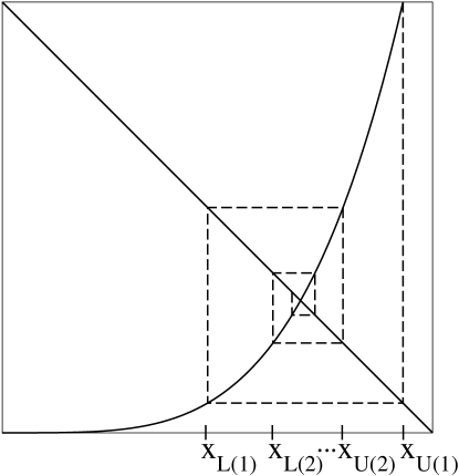
Figure 6: Schematic plot of the recurrence method for getting solution of (51). Solid lines $x^{\frac{1}{1-\eta}}$ and $\beta-x$, dashed line is a construction of a recurrence solution (52) and (53). The plots are in a $\beta\times\beta$ box.

Equation (23) can be solved in the following recursive way. First, one introduces new variables:

$$x=\left(\frac{\hat{t}}{\tau_{Q}}\right)^{2}\ \ ,\ \ \beta=\frac{1}{\alpha^{2}\tau_{Q}^{2}}.$$ (50)

In these variables Equation (23) becomes:

$$x^{\frac{1}{1-\eta}}=\beta-x,$$ (51)

and we assume that $\beta>1$ (diabatic evolutions).

A quick look at Fig. 6, makes clear that the solution can be obtained by considering a series of inequalities, numbered by index $i$, in the form

$$x_{L(i)}<x<x_{U(i)},$$ (52)

where both lower ($x_{L(i)}$) and upper ($x_{U(i)}$) bounds satisfy the the same recurrence equation

$$x_{L,U(i)}=\left[\beta-\left[\beta-x_{L,U(i-1)}\right]^{1-\eta}\right]^{1-\eta},$$ (53)

with the initial conditions $x_{L(0)}=0$, $x_{U(0)}=\beta$. Considering a few iterations one can show that the solution of (51) can be conveniently written as

$$x^{\frac{1}{1-\eta}} = \frac{1}{(\alpha\tau_{Q})^{2}}\left[1-(\alpha\tau)^{2\eta}+(1-\eta)(\alpha\tau_{Q})^{4\eta}+\right.$$ (54)

$$\frac{1}{2}(3\eta-2)(1-\eta)(\alpha\tau_{Q})^{6\eta}+\frac{1}{3}(1-\eta)(1-2\eta)$$

$$(3-4\eta)\left.(\alpha\tau_{Q})^{8\eta}+{\cal O}\left(\tau_{Q}^{10\eta}\right)\right].$$

Using (54), different quantities of interest can be determined, e.g.,

$$\hat{\varepsilon}^{2} = \frac{1}{(\alpha\tau_{Q})^{2\eta}}\left[1-\eta(\alpha\tau_{Q})^{2\eta}+\frac{1}{2}\eta(1-\eta)(\alpha\tau_{Q})^{4\eta}-\right.$$ (55)

$$\frac{1}{3}\eta(1-\eta)(1-2\eta)(\alpha\tau_{Q})^{6\eta}+\frac{1}{8}\eta(1-\eta)$$

$$\left.(1-3\eta)(2-3\eta)(\alpha\tau_{Q})^{8\eta}+{\cal O}\left(\tau_{Q}^{10\eta}\right)\right],$$

$$\hat{t} = \tau_{Q}^{\eta}\alpha^{\eta-1}+{\cal O}\left(\tau_{Q}^{3\eta}\right).$$ (56)

Substitution of $\eta=1/2$ into (55) and (56) reproduces diabatic series expansions of $\hat{\varepsilon}$, $\hat{t}$ from the standard Landau-Zener theory (7).

References

- (1) S. Sachdev, Quantum Phase Transitions (Cambridge University Press, Cambridge UK, 2001).
- (2) W.H. Zurek, U. Dorner, and P. Zoller, Phys. Rev. Lett. 95, 105701 (2005).
- (3) J. Dziarmaga, Phys. Rev. Lett. 95, 245701 (2005).
- (4) A. Polkovnikov, Phys. Rev. B 72, 161201(R) (2005).
- (5) R. Schützhold, Phys. Rev. Lett. 95, 135703 (2005).
- (6) E. Farhi, J. Goldstone, S. Gutmann, J. Lapan, A. Lundgren, and D. Preda, Science 292, 472 (2001); A.M. Childs, E. Farhi, and J. Preskill, Phys. Rev. A 65, 012322 (2002).
- (7) W. Wernsdorfer and R. Sessoli, Science 284, 133 (1999); W. Wernsdorfer et al., J. Appl. Phys. 87, 5481 (2000).
- (8) I. Bloch, Nature Physics 1, 23 (2005).
- (9) B. Damski, Phys. Rev. Lett. 95, 035701 (2005).
- (10) T.W.B. Kibble, J. Phys. A 9, 1387 (1976); Phys. Rep. 67, 183 (1980).
- (11) W.H. Zurek, Nature (London) 317, 505 (1985); Acta Phys. Pol. B 24, 1301 (1993); Phys. Rep. 276, 177 (1996).
- (12) N.D. Antunes, L.M.A. Bettencourt, and W.H. Zurek, Phys. Rev. Lett. 82, 2824 (1999)
- (13) P. Laguna and W.H. Zurek, Phys. Rev. Lett. 78, 2519 (1997); A. Yates and W. H. Zurek, Phys. Rev. Lett. 80, 5477 (1998).
- (14) C. Bauerle, Y.M. Bunkov, S.N. Fisher, H. Godfrin, and G.R. Pickett, Nature (London) 382, 332 (1996); V.M.H. Ruutu et al., Nature (London) 382, 334 (1996).
- (15) M.J. Bowick, L. Chandar, E.A. Schiff, and A.M. Srivastava, Science 263, 943 (1994); I. Chuang, R. Durrer, N. Turok, and B. Yurke, Science 251, 1336 (1991).
- (16) R. Carmi, E. Polturak, and G. Koren, Phys. Rev. Lett. 84 4966 (2000); A. Maniv, E. Polturak, and G. Koren, Phys. Rev. Lett. 91, 197001 (2003).
- (17) R. Monaco, J. Mygind, and R.J. Rivers, Phys. Rev. Lett. 89, 080603 (2002); Phys. Rev. B 67, 104506 (2003). R. Monaco, U.L. Olsen, J. Mygind, R.J. Riviers, and V.P. Koshelets, cond-mat/0503707.
- (18) C. Zener, Proc. R. Soc. A 137, 696 (1932).
- (19) N. D. Antunes, P. Gandra, R.J. Rivers, hep-ph/0504004.
- (20) N. V. Vitanov and B. M. Garraway, Phys. Rev. A 53, 4288 (1996); N. V. Vitanov, Phys. Rev. A 59, 988 (1999).
- (21) E.T. Whittaker and G.N. Watson, A Course of Modern Analysis (Cambridge University Press, Cambridge UK, 1958).