Inter-edge interactions and novel fixed points at a junction of quantum Hall line junctions

Abstract

We show that novel fixed points (characterized by matrices which specify the splitting of the currents at the junction) can be accessed in a system which contains a junction of three quantum Hall line junctions. For such a junction of fractional quantum Hall edge states, we find that it is possible for both the flower (single droplet) and islands (three droplets) configurations to be stable in an intermediate region, for a range of values of the inter-edge repulsive interactions. A measurement of the tunneling conductance as a function of the gate voltage controlling inter-edge repulsions can give a clear experimental signal of this region.

Line junctions renn between the edge states of a fractional quantum Hall system wen allow the realization of one-dimensional systems of interacting electrons with a tunable Luttinger parameter gogolin . A line junction is formed by creating a narrow barrier which divides a fractional quantum Hall liquid (FQHL) such that there are chiral edge states flowing in opposite directions on the two sides of the barrier kang ; roddaro ; the edges interact with each other through Coulomb repulsion. A line junction is thus similar to a non-chiral quantum wire; however, the physical separation between the two edges of the effective non-chiral wire allows for a greater control over the strength of the interaction between them.

Recent experiments have shown that the geometry of the quantum Hall droplet and the location of the points across which tunneling occurs can influence the degree of back-scattering and therefore the transport. Motivated by this, we will study here a FQHL droplet with three narrow barriers as shown in Fig. 1. (Junctions of three quantum Hall edges have been studied earlier chen ; oshikawa ; chamon , but not in the context of line junctions). The width of the narrow barrier between the edges can be tuned to control the Coulomb repulsion between the two edges on its opposite sides; this in turn controls the Luttinger parameter $g$ in each non-chiral wire which is formed by the two edges. Unlike the typical split Hall bar model, this geometry offers access to a new class of tunnelings and fixed points. When there is perfect symmetry between the three barrier gates, we find that there is a range of $g$ for which both the flower fixed point (fully disconnected in terms of wires) and the islands fixed point (chiral in terms of wires) are stable. We compute the scaling of the tunneling conductances around these fixed points.

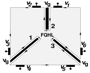
Figure 1: Single droplet (flower configuration) of FQHL. Line junctions are formed by the gate voltages $V_{g}$. $V_{i}$ denote the potentials which drive currents between different edges.

These fixed points are obtained by imposing boundary conditions on the currents via a matrix which splits the currents into the three ‘wires’. Although many consistent (conformally invariant) boundary conditions are possible nayak ; chen ; oshikawa ; chamon , we will focus on certain simple boundary conditions which can be visualized in terms of processes involving the electrons and quasi-particles (quasi-electrons and quasi-holes) at the junction.

The Lagrangian for a system of three quantum Hall line junctions is given by

$$L = {1\over 4\pi}~{}\sum_{i=1}^{3}~{}[~{}\int_{0}^{\infty}dx~{}\partial_{x}\phi_{iO}~{}(-\partial_{t}-v\partial_{x})~{}\phi_{iO}$$ (1)

$$~{}~{}~{}~{}~{}~{}~{}~{}~{}~{}~{}+\int_{-\infty}^{0}dx~{}\partial_{x}\phi_{iI}~{}(-\partial_{t}-v\partial_{x})~{}\phi_{iI}~{}]$$

$$+~{}{v\lambda\over\pi}~{}\sum_{i=1}^{3}~{}\int_{0}^{\infty}dx~{}\partial_{x}\phi_{iO}(x)~{}\partial_{x}\phi_{iI}(-x)~{},$$

where $v$ denotes the velocity, $i$ labels the wire, the incoming fields $\phi_{iI}$ are defined from $x=-\infty$ to $0$, and the outgoing fields $\phi_{iO}$ from $x=0$ to $\infty$. The geometry allows for a screened Coulomb interaction between the left and right movers with a strength $\lambda$ which has to be positive; $\lambda$ can be varied by a gate potential. When the gate potential is large, the left and right movers are well-separated and $\lambda$ is small; when it is small, the two modes move closer to each other and $\lambda$ is large. We restrict ourselves here to the case where there is no hopping between the modes. Note that $\lambda$ is related to the parameter $g$ of a non-chiral Luttinger wire as $g=[(1-\lambda)/(1+\lambda)]^{1/2}$. We therefore choose $\lambda$ to be less than one.

The quasi-electron and electron operators are given by $\psi_{qe}=\eta_{i}e^{i{\sqrt{\nu}}\phi_{i}}$ and $\psi_{el}=\chi_{i}e^{i\phi_{i}/{\sqrt{\nu}}}$ respectively, where $\nu~{}(=1/3,1/5,\cdots)$ is the FQHL filling, and $\eta_{i}$ and $\chi_{i}$ are the Klein factors for quasi-electrons and electrons respectively. The density fields canonically conjugate to $\phi$ are given by $\rho_{i,I/O}=-(1/2\pi)\partial_{x}\phi_{i,I/O}$, so that

$${}[\phi_{iI/O}(x),\rho_{jI/O}(y)] = \delta_{ij}~{}\delta(x-y)~{}~{}{\rm for}~{}~{}x,y</>0~{},$$

$${}[\phi_{iI}(x),~{}\rho_{j0}(y)] = 0~{}~{}{\rm for}~{}~{}x<0,~{}y>0~{}.$$ (2)

At the junction, the Lagrangian in Eq. (1) must be supplemented by boundary conditions which ensure that the current (given by $j_{i,I/O}=(1/2\pi)\partial_{t}\phi_{i,I/O}$) is conserved, and that Eqs. (2) are satisfied. This implies that the fields must be related at the junction as ${\vec{\phi}}_{O}=S{\vec{\phi}}_{I}$, where the $3\times 3$ splitting matrix $S$ is real and orthogonal, and each of its columns (or rows) add up to 1. The latter conditions ensure that the fields satisfy $\sum\phi_{iO}=\sum_{i}\phi_{iI}$, so that the current is conserved at the junction.

We now consider some simple forms of $S$, which are the identity matrix $I$ and the two chiral matrices, namely, $M_{+}$ with $M_{13}=M_{21}=M_{32}=1$ and all the other matrix elements equal to zero, and $M_{-}=M_{+}^{T}$. For a given sign of the magnetic field, only one chirality is possible, so we only consider one of them, say, $M_{+}$. We will consider a given value of the FQHL filling $\nu<1$, and study the scaling dimensions of various tunneling operators as functions of $\lambda$ or the Luttinger parameter $g$.

The case $S=I$ corresponds to the situation in Fig. 1, in which current from the incoming edge $i$ goes entirely to the outgoing edge $i$. Since there is only one droplet, one can consider both electron and quasi-particle tunneling between two edges, say, between the incoming edge 1 and the outgoing edge 2. The scaling dimensions of this operator can be computed after performing a Bogoliubov diagonalization given by $\phi^{\prime}_{O/I}=[(1+g)\phi_{iO/I}+(1-g)\phi_{I/O}]/2\sqrt{g}$ in each wire. We find that the tunneling operator as described above has the scaling dimension $\nu/g$ for quasi-particles and $1/(\nu g)$ for electrons. Since $\nu$ and $g$ are both less than 1, electron tunneling is irrelevant in the sense of the renormalization group (RG). However, if $g>\nu$, quasi-particle tunneling is relevant, and the configuration in Fig. 1 is unstable under an RG flow. In that case, since tunneling between the incoming edge $i$ and the outgoing edge $i+1$ grows, it is reasonable to assume that the configuration in Fig. 1 flows, at long distances, to the one in Fig. 2. [Note that in the absence of Coulomb interaction between the edges, $g=1$ is greater than $\nu$; hence the configuration in Fig. 1 is unstable to Fig. 2. This agrees with the usual expectation that a single FQHL droplet is unstable to the formation of multiple droplets.]

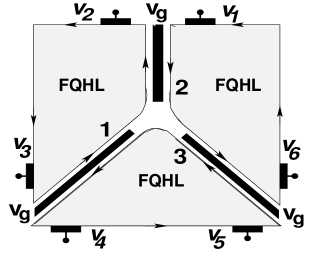
Figure 2: Three droplets (islands configuration) of FQHL. The gate voltages and potentials are defined as in Fig. 1.

The case $S=M_{+}$ corresponds to Fig. 2. In this case, only electrons can tunnel between, say, the incoming edge 1 and the outgoing edges 1 or 3; the conservation of charge (in integer multiples of an electron) in the individual droplets prevents tunneling of quasi-particles from the incoming edge 1 to the outgoing edges 1 and 3. To calculate the scaling dimension of the tunneling operator, we first carry out the Bogoliubov diagonalization in each wire and then rewrite the boundary condition in terms of the free incoming and outgoing fields, i.e.,

$${\vec{\phi}^{\prime}}_{O}~{}=~{}\frac{(1+g)S+(1-g)I}{(1+g)I+(1-g)S}~{}{\vec{\phi}^{\prime}}_{I}~{}.$$ (3)

The scaling dimension of the electron tunneling operator between any incoming edge and outgoing edge is then found to be $4g/[\nu(3+g^{2})]$. Note that we reproduce the scaling dimensions obtained in Refs. oshikawa ; chamon near the chiral fixed points, without using Klein factors or mapping to the dissipative Hofstader model. This is because we compute the scaling dimension of weak tunneling directly at the islands fixed point of Fig. 2, rather than studying the strong tunneling limit (with multiple hoppings involving Klein factors) of the flower fixed point of Fig. 1. Thus we identify the islands configuration (and its time-reversed form) with $\chi_{\pm}$ oshikawa ; chamon . (For $g$ close to 1, these reduce to the chiral fixed points first studied in Ref. lal ).

We find that the dimension of the electron tunneling operator at the chiral fixed point is less than 1 if $g<g_{c}$, where $g_{c}=\frac{2}{\nu}-{\sqrt{\frac{4}{\nu^{2}}-3}}$; this is equal to $0.255$ for $\nu=1/3$ (this value of $g$ corresponds to $\lambda=0.877$). Hence the configuration in Fig. 2 is unstable if $g<g_{c}$ and stable if $g>g_{c}$. For $g<g_{c}$, since tunneling between the incoming edge 1 and the outgoing edge 1 grows, it is reasonable to assume that Fig. 2 flows under RG to Fig. 1. We thus see that the flower in Fig. 1 is stable if $g<\nu$, and the islands in Fig. 2 is stable if $g>g_{c}$. Since $g_{c}$ is less than $\nu$ (for $\nu<1$), we have the interesting situation that in the intermediate range $g_{c}<g<\nu$, the configurations in Figs. 1 and 2 are both stable; this implies that there must be an unstable fixed point lying between the two configurations. As a function of the gate voltage controlling the strength of the inter-edge interactions, the single droplet is unstable to breaking up into three droplets if the inter-edge coupling $\lambda<0.877$. But if the gate voltage is decreased and the inter-edge interaction increases to $\lambda>0.877$, the single droplet configuration becomes stable. These results are summarized in the table below.

Geo-	Tunneling	Scaling	RG relevance
metry	Operator	dimen-	$g<g_{c}$	$g_{c}<g$	$g>\nu$
		sion		$<\nu$
Flower	$e^{i(\phi_{iO}-\phi_{jI})/{\sqrt{\nu}}}$	$\frac{1}{\nu g}$	irrel.	irrel.	irrel.
Flower	$e^{i\sqrt{\nu}(\phi_{iO}-\phi_{jI})}$	$\frac{\nu}{g}$	irrel.	irrel.	rel.
Islands	$e^{i(\phi_{iO}-\phi_{jI})/{\sqrt{\nu}}}$	$\frac{4g}{\nu(3+g^{2})}$	rel.	irrel.	irrel.

One way to experimentally distinguish between the flower and islands configurations would be to measure the differential tunneling conductance $dI/dV$ between, say, the incoming edge 1 and the outgoing edge 3; the tunneling amplitude for this process is expected to be small in both configurations since those two edges are well separated. The tunneling conductance $G\sim b^{2}V^{2(d-1)}$ where $V$ is the voltage difference (or temperature $T^{2(d-1)}$) for small values of $V$ (or $T$), where $d$ is the scaling dimension of the tunneling operator, and $b$ is the back-scattering strength. For the flower which is stable if $g<\nu$, tunneling will be dominated by quasi-particles since the value of $d$ is smaller for them than for electrons; the exponent of $V$ (or $T$) will be given by $(2\nu/g)-2$. For the islands which is stable if $g>g_{c}$, only electrons can tunnel, and the exponent of $V$ will be given by $8g/[\nu(3+g^{2})]-2$. Note that the change from instability to stability occurs at different points for the two configurations, which is why there is an intermediate region where both configurations are stable. In Fig. 3, we plot the tunneling conductances for both configurations in the three regions (i), (ii) and (iii) defined in the caption.

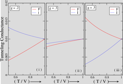
Figure 3: Tunneling conductance in regions (i) $0<g<g_{c}$, (ii) $g_{c}<g<\nu$, and (iii) $\nu<g<1$ as a function of the voltage or temperature, for the flower (F) and islands (I) configurations. The quasi-particle tunneling is plotted for the flower, and electron tunneling for the islands. The conductance has been normalized to $0.01$ at the temperature $T=1$ (scaled by the cutoff temperature $\Lambda$). The flower and islands configurations are both stable in region (ii).

If we start with the flower configuration with $g$ slightly less than 1 (weak back-scattering) at high temperatures (or high voltages), and slowly reduce the temperature, the system flows to the islands configuration. The tunneling conductance at low temperatures (governed by electron tunneling) is plotted in Fig. 4 (line F-I, signifying that we start with the flower configuration at high temperatures and reach the islands configuration at low temperatures). The experiment can be repeated after reducing $g$. Until we reach $g=1/3$, the system always flows to the islands configuration at low temperatures and the tunneling conductance is governed by the F-I line. However, for $g<1/3$, the flower configuration is stable; even at low temperatures, the system remains in that configuration. The tunneling conductance at low temperatures is governed by quasi-particle tunneling plotted in Fig. 4 as the line F-F. Note that at $g=1/3$, the electron and quasi-particle tunneling operators are both marginal.

Similarly, we may start with the islands configuration at high temperatures and look at the scaling of the conductance at low temperatures. Until we reach $g=g_{c}$, the islands remains stable and the low temperature tunneling conductance is governed by the irrelevant electron operator (which turns marginal at $g_{c}$). If the experiment is repeated with $g<g_{c}$, the low temperature stable phase is the flower configuration, where the conductance is governed by the quasi-particle tunneling operator.

Hence, by starting with either the flower or the islands configuration at high temperatures and changing the value of $g$ of the line junction, we should see a dramatic change in the behaviors of the tunneling conductances at $g=\nu$ and $g=g_{c}$. This is an unambiguous prediction which can be experimentally tested.

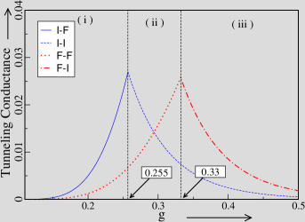
Figure 4: Tunneling conductance as a function of $g$, starting from either the islands configuration (I-I and I-F lines) or flower configuration (F-F and F-I lines) at high temperature. The conductance at the marginal points has been normalized to be 0.025. Low temperature ($T=0.1$) conductances (quasi-particle tunneling for the I-F and F-F lines, and electron tunneling for the I-I and F-I lines) have been plotted.

The three droplet and the single droplet configurations will also show different behaviors of the noise noise ; safi . The shot noise at the lowest temperatures will show signatures of both electron and quasi-particle hopping for the single droplet case, and a signature of only electron hopping for the three droplet configuration. The zero-frequency limit of the shot noise $S(\omega)$ is proportional to the tunneling current $I$ and to the charge of the electron/quasi-particle which is tunneling; the term of order $\omega$ in $S(\omega)$ is proportional to $V^{4(d-1)}$ noise .

For a general $S$-matrix at the boundary, we can study the problem by solving the equations of motion following from the Lagrangian in Eq. (1); details will be reported elsewhere das2 . [Here, the splitting matrix and the interactions are introduced at the same time. This is different in spirit from the procedure of ‘delayed boundary condition’ followed in Ref. oshikawa , where the boundary conditions are chosen a posteriori.] We find that for each wave number $k$, there are three modes (labeled by $p=1,2,3$) with the same velocity $\tilde{v}=v{\sqrt{1-\lambda^{2}}}$. Upon imposing the commutation relations given in Eq. (2), we obtain

$$\phi_{iI/O}(x,t)~{}=~{}\int_{0}^{\infty}~{}\frac{dk}{\sqrt{k}}~{}\sum_{p}~{}\psi_{ipI/O,k}(x,t)~{},$$

$$\psi_{ipI/O,k}~{}=~{}\alpha_{pk}~{}(a_{ipI/O}e^{ikx}+b_{ipI/O}e^{-ikx})~{}e^{-i\tilde{v}kt}$$

$$~{}~{}~{}~{}~{}~{}~{}~{}~{}~{}~{}~{}~{}~{}~{}+~{}{\rm h.c.}~{},$$

$${\rm with}~{}~{}[\alpha_{pk}~{},~{}\alpha_{p^{\prime}k^{\prime}}^{\dagger}]~{}=~{}\pi~{}\delta_{pp^{\prime}}~{}\delta(k-k^{\prime})~{}.$$ (4)

The wave function coefficients $a_{ip,I/O}$ and $b_{ip,I/O}$ may be compactly written as $3\times 3$ matrices $A_{I/O}$ and $B_{I,O}$, such that $(A_{I/O})_{ip}=a_{ip,I/O}$ and $(B_{I/O})_{ip}=b_{ip,I/O}$. In the absence of interactions, the incident waves are given by $A_{I}=I$, and the transmitted waves by $A_{O}=S$; the reflected waves $B_{I}$ and $B_{O}$ vanish. The interactions cause rescaling and reflections of the waves in each wire; this is governed by a parameter $\mu={\lambda}/{(1+{\sqrt{1-\lambda^{2}}})}$, which is related to the parameter $g$ as $\mu=(1-g)/(1+g)$. Furthermore, the boundary $S$ matrix relates the transmitted waves to the incident waves. We find that

$$A_{I}=\frac{I}{\sqrt{1-\mu^{2}}}~{}, B_{I}=\mu~{}D~{}A_{I}~{},$$

$$A_{O}=D~{}A_{I}~{}, B_{O}=\mu A_{I}~{},$$ (5)

where $D={(S-\mu I)}/{(I-\mu S)}$ is an orthogonal matrix.

We can now compute the dimension of an operator which produces tunneling at the junction ($x=0$) between an incoming edge $i$ and an outgoing edge $j$. The tunneling operator is given by $O_{\beta,ij}(t)=\exp i\beta(\phi_{iI}(0,t)-\phi_{jO}(0,t))$, where $\beta={\sqrt{\nu}}$ and $1/{\sqrt{\nu}}$ for quasi-electrons and electrons respectively. In terms of the matrices $A$ and $B$ given in Eq. (5), the scaling dimension of $O_{ij}$ is given by

$$d_{\beta,ij} = \frac{\beta^{2}}{2}~{}\sum_{p}~{}(A_{I,ip}~{}+~{}B_{I,ip}~{}-~{}A_{O,jp}~{}-~{}B_{O,jp})^{2}$$ (6)

$$= \frac{\beta^{2}}{1-\mu^{2}}~{}[~{}1~{}-~{}D_{ji}~{}+~{}\mu~{}(~{}D_{ii}~{}+~{}D_{jj}~{}-~{}2\delta_{ij}~{})$$

$$~{}~{}~{}~{}~{}~{}~{}~{}~{}~{}~{}+~{}\mu^{2}~{}(~{}1~{}-~{}D_{ij}~{})~{}]~{}.$$

For instance, for the electron hopping operator at the fixed point $M_{+}$, this gives $d=4g/\nu(3+g^{2})$, which agrees with the earlier analysis. This formalism can be used to check the stability of various other fixed points das2 .

In summary, we have proposed a new geometry for line junctions of FQHL edges. For $\nu=1/3$, we find that for values of the parameter $g$ (which is determined by the width or gate voltage of the line junction) lying in the range $0.255<g<0.333$, the single droplet (flower) and the three droplet (islands) phases are both stable. These phase boundaries can be experimentally tested by measuring the voltage power law as a function of the gate voltage which controls $g$.

We thank Siddhartha Lal for interesting discussions. SD acknowledges many stimulating and useful discussions with Yuval Gefen. SD was supported by the Feinberg Graduate School, Israel, and is also grateful to HRI for hospitality during the completion of this work. DS thanks the Department of Science and Technology, India for financial support under projects SR/FST/PSI-022/2000 and SP/S2/M-11/2000.

References

- (1) S. R. Renn and D. P. Arovas, Phys. Rev. B51, 16832 (1995); C. L. Kane and M. P. A. Fisher, Phys. Rev. B56, 15231 (1997); A. Mitra and S. M. Girvin, Phys. Rev. B64, 041309 (2001); M. Kollar and S. Sachdev, Phys. Rev. B65, 121304 (2002); E.-A. Kim and E. Fradkin, Phys. Rev. B67, 045317 (2003); U. Zülicke and E. Shimshoni, Phys. Rev. B69, 085307 (2004), and Phys. Rev. Lett. 90, 026802 (2003); E. Papa and A. H. MacDonald, Phys. Rev. Lett. 93, 126801 (2004).
- (2) X.-G. Wen, Phys. Rev. B44, 5708 (1991); Phys. Rev. B41, 12838 (1990).
- (3) A. O. Gogolin, A. A. Nersesyan, and A. M. Tsvelik, Bosonization and Strongly Correlated Systems (Cambridge University Press, Cambridge, 1998); T. Giamarchi, Quantum Physics in One Dimension (Oxford University Press, Oxford, 2004); S. Rao and D. Sen, in Field Theories in Condensed Matter Physics, edited by S. Rao (Hindustan Book Agency, New Delhi, 2001).
- (4) W. Kang, H. L. Stormer, L. N. Pfeiffer, K. W. Baldwin, and K. W. West, Nature 403, 59 (2000); I. Yang, W. Kang, K. W. Baldwin, L. N. Pfeiffer, and K. W. West, Phys. Rev. Lett. 92, 056802 (2004); I. Yang, W. Kang, L. N. Pfeiffer, K. W. Baldwin, K. W. West, E.-A. Kim, and E. Fradkin, Phys. Rev. B71, 113312 (2005).
- (5) S. Roddaro, V. Pellegrini, F. Beltram, G. Biasiol, and L. Sorba, Phys. Rev. Lett. 93, 046801 (2004); S. Roddaro, V. Pellegrini, F. Beltram, G. Biasiol, L. Sorba, R. Raimondi, and G. Vignale, Phys. Rev. Lett. 90, 046805 (2003).
- (6) S. Chen, B. Trauzettel, and R. Egger, Phys. Rev. Lett. 89, 226404 (2002); R. Egger, B. Trauzettel, S. Chen, and F. Siano, New Journal of Physics 5, 117 (2003).
- (7) M. Oshikawa, C. Chamon, and I. Affleck, cond-mat/0509675.
- (8) C. Chamon, M. Oshikawa, and I. Affleck, Phys. Rev. Lett. 91, 206403 (2003).
- (9) C. Nayak, M. P. A. Fisher, A. W. W. Ludwig, and H. H. Lin, Phys. Rev. B59, 15694 (1999).
- (10) S. Lal, S. Rao, and D. Sen, Phys. Rev. B66, 165327 (2002).
- (11) Manuscript under preparation.
- (12) C. de C. Chamon, D. E. Freed, and X. G. Wen, Phys. Rev. B53, 4033 (1996) and Phys. Rev. B51, 2363 (1995).
- (13) I. Safi, P. Devillard, and T. Martin, Phys. Rev. Lett. 86, 4628 (2001); E.-A. Kim, M. Lawler, S. Vishveshwara, and E. Fradkin, Phys. Rev. Lett. 95, 176402 (2005).