Unified phase diagram of models exhibiting neutral-ionic transition

Abstract

We have studied the neutral-ionic transition in organic mixed-stack compounds. A unified model has been derived which, in limiting cases, is equivalent to the models proposed earlier, the donor-acceptor model and the ionic Hubbard model. Detailed numerical calculations have been performed on this unified model with the help of the density-matrix renormalization-group (DMRG) procedure calculating excitation gaps, ionicity, lattice site entropy, two-site entropy, and the dimer order parameter on long chains and the unified phase diagram has been determined.

I Introduction

Two physically seemingly different models have been proposed in the literature to describe the neutral-ionic (N-I) transition first observed in organic mixed-stack charge-transfer salts.torr_01 ; torr_02 Assuming that the coupling between the stacks is weak, the system is modelled as a linear chain in which two kinds of molecules alternate. Assuming furthermore, that it is sufficient to consider a single orbital per site, Torrance and Hubbard hubb-torr have suggested that the different nature of the two molecules can be attributed to different values of the on-site energy, while the on-site Coulomb repulsion $U$ can be taken to be identical. Taking into account the finite transfer integral between neighboring molecules we are led to the so-called ionic Hubbard model described by the Hamiltonian

$$\begin{split}{\mathcal{H}}&=t\sum_{i\sigma}\left(c^{\dagger}_{i\sigma}c^{\phantom{\dagger}}_{i+1\sigma}+c^{\dagger}_{i+1\sigma}c^{\phantom{\dagger}}_{i\sigma}\right)\\ &\phantom{=}+U\sum_{i}n_{i\uparrow}n_{i\downarrow}+\frac{\Delta}{2}\sum_{i}(-1)^{i}n_{i}\,,\end{split}$$ (1)

where $c^{\dagger}_{i\sigma}(c^{\phantom{\dagger}}_{i\sigma})$ is the usual creation (annihilation) operator of electrons at site $i$ with spin $\sigma$, $n_{i\sigma}=c^{\dagger}_{i\sigma}c^{\phantom{\dagger}}_{i\sigma}$ and $n_{i}=\sum_{\sigma}n_{i\sigma}$ is the occupation number at site $i$.

When the number of electrons is exactly equal to the number of sites, the competition between the on-site energy difference $\Delta$ and the Coulomb energy $U$ will determine whether the system is a band insulator (BI) or a correlated Mott insulator (MI). It is easily seen by looking at the energy levels in the atomic limit, shown in Fig. 1, that if hopping processes can be neglected, it is energetically favorable to have doubly occupied odd sites and empty even sites when $U<\Delta$ (the energy of the pair is $E=U-\Delta<0$), while in the opposite case ($U>\Delta$) in the lowest-energy configuration every site is occupied by one electron (the energy of such a pair is $E=0$), but their spin can be arbitrarily oriented. In the band-insulator state both the charge and spin gaps are finite, while in the correlated Mott insulator only the charge gap is finite. The transition between these phases takes place at $U=\Delta$.

$U<\Delta$		$U>\Delta$

Figure 1: Energy levels of the ionic Hubbard model in the atomic limit for $U<\Delta$ and $U>\Delta$.

As was first pointed out by Fabrizio et al.,fabri for finite values of the hopping integral $t$ the transition between these two states occurs in two steps. The charge gap closes at a critical value $U_{\rm c1}$, but it reopens immediately, while the spin gap vanishes at a different value $U_{\rm c2}>U_{\rm c1}$. The transition at $U=U_{\rm c1}$ is of Ising-like while the one at $U_{\rm c2}$ is a Berezinskii-Kosterlitz-Thouless (BKT) transition. A dimerized bond-order (BO) phase exists between the two critical values.

Since then the model has been studied in detail by several groups using both analytic and numerical methods. The most recent works are in Refs. [torio, ; zhang, ; kampf, ; manma, ; soos, ; aligia, ; leo, ; legeza, ] where further references can be found. After some controversy, by now consensus seems to emerge, the numerical resultsmanma ; leo ; legeza seem to support the picture with two transitions. The model has also been extended to include intersite Coulomb interaction bruins ; aligia with rather similar results.

In realistic charge-transfer salts, however, the intramolecular Coulomb energy is presumably the largest energy and it is reasonable to assume that its unique role is to forbid doubly ionized molecules. If that is so, the transition between the neutral and ionic phases is driven by other couplings. In the model studied in detail by Avignon et al.,avignon Girlando and Painelli,girlando and Horovitz and one of the authors horovitz it is assumed that donor and acceptor molecules alternate along the chain. In its neutral state (D⁰), the highest occupied molecular orbital (HOMO) of the donor is filled by two electrons of opposite spin. The ionization energy to remove an electron from this orbital and to create thereby a singly ionized D⁺ donor is $I$. Taking into account the Coulomb repulsion $U_{\rm D}$ the energy of the doubly ionized (D²⁺) state is $2I+U_{\rm D}$. The donor molecules can thus be described by the Hamiltonian

$$\begin{split}{\mathcal{H}}_{\rm D}&=I\rule{-5.69054pt}{0.0pt}\sum_{\rm donor\,sites}\rule{-5.69054pt}{0.0pt}(2-n_{i})\\ &\phantom{=,}+U_{\rm D}\rule{-5.69054pt}{0.0pt}\sum_{\rm donor\,sites}\rule{-5.69054pt}{0.0pt}(1-n_{i\uparrow})(1-n_{i\downarrow})\,.\end{split}$$ (2)

The energies are measured with respect to the neutral configuration. If $U_{\rm D}\gg I$, its role is to forbid doubly ionized sites, empty donor orbitals.

On the other hand the lowest unoccupied molecular orbital (LUMO) of the acceptor is empty in its neutral state (A⁰). The energy is lowered to $-A$, where $A$ is the affinity, when the level becomes singly occupied, singly ionized (A^-), while the doubly ionized (A^2-) acceptors have a high energy due to the Coulomb repulsion $U_{\rm A}$. The acceptor molecules are described by the Hamiltonian

$${\mathcal{H}}_{\rm A}=-A\rule{-5.69054pt}{0.0pt}\sum_{\rm acceptor\,sites}\rule{-5.69054pt}{0.0pt}n_{i}+U_{\rm A}\rule{-5.69054pt}{0.0pt}\sum_{\rm acceptor\,sites}\rule{-5.69054pt}{0.0pt}n_{i\uparrow}n_{i\downarrow}\,.$$ (3)

If $U_{\rm A}\gg A$, its role is to forbid doubly ionized sites, doubly occupied acceptor orbitals. The atomic energy levels of the donor and acceptor molecules are shown schematically in Fig. 2.

Figure 2: Atomic energy levels of donor and acceptor molecules.

Since $I$ and $A$ are fixed internal parameters of the molecules, and it is assumed that $I-A>0$, the molecules are neutral in the ground state of the stack unless a transition to an ionized state is driven by the intermolecular Coulomb attraction $V$ between the oppositely ionized donors (D⁺) and acceptors (A^-),

$$\begin{split}{\mathcal{H}}_{\rm C}&=-V\rule{-5.69054pt}{0.0pt}\sum_{\rm donor\,sites}\rule{-5.69054pt}{0.0pt}(2-n_{i})n_{i+1}\\ &\phantom{=,}-V\rule{-5.69054pt}{0.0pt}\sum_{\rm acceptor\,sites}\rule{-5.69054pt}{0.0pt}n_{i}(2-n_{i+1})\,.\end{split}$$ (4)

In this atomic limit this transition should occur at $V=I-A$.

However, in addition to these terms one has to take into account the charge transfer between the donor and acceptor molecules described by

$${\mathcal{H}}_{\rm CT}=t\rule{-5.69054pt}{0.0pt}\sum_{{\rm all\,sites,\,}\sigma}\rule{-5.69054pt}{0.0pt}\left(c^{\dagger}_{i\sigma}c^{\phantom{\dagger}}_{i+1\sigma}+c^{\dagger}_{i+1\sigma}c^{\phantom{\dagger}}_{i\sigma}\right)\,.$$ (5)

Since for finite hopping the molecules are always at least partially ionized, this may smear out the sharp transition between the neutral and ionic phases.

In fact, exact diagonalization on relatively short chains horovitz and valence-bond calculations soos-maz ; girlando indicated that the transition remains of first order until $t\leq 0.15(I-A)$. For larger $t$ values a second-order or BKT-like transition was observed. The charge, spin and charge-transfer gaps seemed to vanish at the same critical intermolecular Coulomb coupling $V_{\rm c}$, but the charge gap reopens again.

Not only the interaction driving the neutral-ionic transition is different in the two models but also the character of the transition seems to be different. The aim of the present work is to perform a more careful study of the neutral-ionic transition. First it is shown that a unified model can be derived which is identical to the donor-acceptor model in the limit when the intramolecular Coulomb repulsion forbids doubly ionized donors and acceptors, and at the same time it is also a good approximation to the ionic Hubbard model when $t\ll\Delta$, but $U-\Delta$ can be arbitrary. Detailed numerical calculations are performed on this unified model with the help of the density-matrix renormalization-group (DMRG) white procedure calculating excitation gaps, ionicity, single-site entropy, two-site entropy, and the dimer order parameter on long chains and the unified phase diagram is determined.

The setup of the paper is as follows. In Sec. II we transform the Hamiltonian of the two models into an effective spin-1 model and show their relationship. In Sec. III we discuss how the quantum phase transition between the neutral and ionic phases can be best described and our numerical procedure is presented. The results are given in Sec. IV, and the conclusions are drawn in Sec. V.

II Unified spin-1 Hamiltonian

As mentioned earlier, in the donor-acceptor model, the on-site Coulomb couplings are large compared to the other characteristic energies in the problem, and the limit $U_{\rm D},\,U_{\rm A}\rightarrow\infty$ can be taken whereby the doubly ionized molecular states (empty donor D²⁺ and doubly occupied acceptor A^2-) are forbidden. Since only three states per site survive, this model can be mapped onto an effective $S=1$ spin model.horovitz The appropriate mapping between the allowed electronic states and spin states is shown in Fig. 3.

$\left|\,0\,\right>$ $\longrightarrow$ excluded $\left|\,\uparrow\,\right>$ $\longrightarrow$ $\left|\,1\,\right>$ $\left|\,\downarrow\,\right>$ $\longrightarrow$ $\left|\,-1\,\right>$ $\left|\,\uparrow\downarrow\,\right>$ $\longrightarrow$ $\left|\,0\,\right>$		$\left|\,0\,\right>$ $\longrightarrow$ $\left|\,0\,\right>$ $\left|\,\uparrow\,\right>$ $\longrightarrow$ $\left|\,1\,\right>$ $\left|\,\downarrow\,\right>$ $\longrightarrow$ $\left|\,-1\,\right>$ $\left|\,\uparrow\downarrow\,\right>$ $\longrightarrow$ excluded
Donor		Acceptor

Figure 3: Mapping of the allowed electronic states of donor and acceptor molecules to $S=1$ spin states.

As is seen, the transfer of an electron with spin $\uparrow$ or $\downarrow$ from the neutral donor at site $2j-1$ to the empty, neutral acceptor at site $2j$, the process D${}_{2j-1}^{0}$A${}_{2j}^{0}\rightarrow$ D${}_{2j-1}^{+}$A${}_{2j}^{-}$ corresponds in the spin language to an exchange process $\left|0\right>_{2j-1}\left|0\right>_{2j}\rightarrow\left|-1\right>_{2j-1}\left|1\right>_{2j}$ or $\left|0\right>_{2j-1}\left|0\right>_{2j}\rightarrow\left|1\right>_{2j-1}\left|-1\right>_{2j}$. The opposite processes are also possible. No hopping could, however, take place between a neutral donor and an ionized acceptor or an ionized donor and a neutral acceptor or between ionized neighbors when the spins of the electrons are parallel.

However, one has to take into account that due to the fermionic nature of the electrons, these hopping processes appear with different signs. Acting by the charge-transfer term on a neutral donor-acceptor pair

$$\begin{split}{\mathcal{H}}_{\rm CT}&\,c_{2j-1\uparrow}^{\dagger}c_{2j-1\downarrow}^{\dagger}|0\rangle_{2j-1}|0\rangle_{2j}\\ =&\,t\big{(}c_{2j-1\uparrow}^{\dagger}c_{2j\downarrow}^{\dagger}-c_{2j-1\downarrow}^{\dagger}c_{2j\uparrow}^{\dagger}\big{)}|0\rangle_{2j-1}|0\rangle_{2j}\\ =&\,t\big{(}|\!\uparrow\rangle_{2j-1}|\!\downarrow\rangle_{2j}-|\!\downarrow\rangle_{2j-1}|\!\uparrow\rangle_{2j}\big{)}\,.\end{split}$$ (6)

Similarly when the charge-transfer term acts on an A${}_{2j}^{0}$D${}_{2j+1}^{0}$ pair

$$\begin{split}{\mathcal{H}}_{\rm CT}&\,|0\rangle_{2j}c_{2j+1\uparrow}^{\dagger}c_{2j+1\downarrow}^{\dagger}|0\rangle_{2j+1}\\ =&\,t\big{(}c_{2j\uparrow}^{\dagger}c_{2j+1\downarrow}^{\dagger}-c_{2j\downarrow}^{\dagger}c_{2j+1\uparrow}^{\dagger}\big{)}|0\rangle_{2j}|0\rangle_{2j+1}\\ =&\,t\big{(}|\!\uparrow\rangle_{2j}|\!\downarrow\rangle_{2j+1}-|\!\downarrow\rangle_{2j}|\!\uparrow\rangle_{2j+1}\big{)}\,.\end{split}$$ (7)

The charge-transfer processes can thus be described in the spin language by the Hamiltonian

$$\begin{split}{\cal H}_{\rm CT}&=-{\textstyle\frac{1}{2}}t\rule{-5.69054pt}{0.0pt}\sum_{\rm all\,sites}\rule{-5.69054pt}{0.0pt}S^{z}_{i}S^{z}_{i+1}\left(S^{+}_{i}S^{-}_{i+1}-S^{-}_{i}S^{+}_{i+1}\right)\\ &\phantom{=,}+{\textstyle\frac{1}{2}}t\rule{-5.69054pt}{0.0pt}\sum_{\rm all\,sites}\rule{-5.69054pt}{0.0pt}\left(S^{+}_{i}S^{-}_{i+1}-S^{-}_{i}S^{+}_{i+1}\right)S^{z}_{i}S^{z}_{i+1}\,,\end{split}$$ (8)

where $S^{+}_{i}$ and $S^{-}_{i}$ are the usual raising and lowering operators corresponding in the fermionic picture to removing or adding an electron. $S^{z}_{i}$ measures the state of the ion, and the product $S^{z}_{i}S^{z}_{i+1}$ makes sure that no charge transfer takes place between a neutral and an ionized site.

Using the commutation relations of the spin operators, this part of the Hamiltonian can be written in the form

$$\begin{split}{\mathcal{H}}_{\rm CT}&=-{\textstyle\frac{1}{2}}t\sum_{i}S_{i}^{z}\left(S_{i}^{+}S_{i+1}^{-}+S_{i}^{-}S_{i+1}^{+}\right)\\ &\phantom{=,}-{\textstyle\frac{1}{2}}t\sum_{i}\left(S_{i}^{+}S_{i+1}^{-}+S_{i}^{-}S_{i+1}^{+}\right)S_{i+1}^{z}\,.\end{split}$$ (9)

It is easy to check that the same matrix elements are obtained if the other terms of the Hamiltonian are written in the spin language as

$$\begin{split}{\cal H}_{\rm D}&=I\rule{-5.69054pt}{0.0pt}\sum_{\rm donor\,sites}\rule{-5.69054pt}{0.0pt}(S^{z}_{i})^{2}\,,\\ {\cal H}_{\rm A}&=-A\rule{-5.69054pt}{0.0pt}\sum_{\rm acceptor\,sites}\rule{-5.69054pt}{0.0pt}(S^{z}_{i})^{2}\,,\\ {\cal H}_{\rm C}&=-V\rule{-5.69054pt}{0.0pt}\sum_{\rm all\,sites}\rule{-5.69054pt}{0.0pt}(S^{z}_{i})^{2}(S^{z}_{i+1})^{2}\,.\end{split}$$ (10)

Due to charge conservation

$$\sum_{\rm donor\,sites}(S^{z}_{i})^{2}=\sum_{\rm acceptor\,sites}(S^{z}_{i})^{2}\,,$$ (11)

and therefore

$${\cal H}_{\rm D}+{\mathcal{H}}_{\rm A}={\textstyle\frac{1}{2}}(I-A)\sum_{\rm all\,sites}(S^{z}_{i})^{2}\,.$$ (12)

We mention that the effective spin-1 Hamiltonian used in Ref. [horovitz, ] differs somewhat from the one given above. The charge-transfer term was written in the form

$$\begin{split}{\cal H}_{\rm CT}&=-{\textstyle\frac{1}{2}}t\rule{-5.69054pt}{0.0pt}\sum_{\rm all\,sites}\rule{-5.69054pt}{0.0pt}S^{z}_{i}S^{z}_{i+1}\left(S^{-}_{i}S^{+}_{i+1}+S^{+}_{i}S^{-}_{i+1}\right)\\ &\phantom{=,}-{\textstyle\frac{1}{2}}t\rule{-5.69054pt}{0.0pt}\sum_{\rm all\,sites}\rule{-5.69054pt}{0.0pt}\left(S^{-}_{i}S^{+}_{i+1}+S^{+}_{i}S^{-}_{i+1}\right)S^{z}_{i}S^{z}_{i+1}\,.\end{split}$$ (13)

The two expressions can be related by a unitary transformation, by introducing phase factors in the mapping, which alternate with a four-site periodicity. The appropriate mapping is given in Fig. 4.

$\left|\,0\,\right>$ $\longrightarrow$ excluded $\left|\,\uparrow\,\right>$ $\longrightarrow$ $\left|\,1\,\right>$ $\left|\,\downarrow\,\right>$ $\longrightarrow$ $\left|\,-1\,\right>$ $\left|\,\uparrow\downarrow\,\right>$ $\longrightarrow$ $\left|\,0\,\right>$		$\left|\,0\,\right>$ $\longrightarrow$ $\phantom{-}\left|\,0\,\right>$ $\left|\,\uparrow\,\right>$ $\longrightarrow$ $-\left|\,1\,\right>$ $\left|\,\downarrow\,\right>$ $\longrightarrow$ $\phantom{-}\left|\,-1\,\right>$ $\left|\,\uparrow\downarrow\,\right>$ $\longrightarrow$ excluded
Donor at site $4j-3$		Acceptor at site $4j-2$
$\left|\,0\,\right>$ $\longrightarrow$ excluded $\left|\,\uparrow\,\right>$ $\longrightarrow$ $-\left|\,1\,\right>$ $\left|\,\downarrow\,\right>$ $\longrightarrow$ $-\left|\,-1\,\right>$ $\left|\,\uparrow\downarrow\,\right>$ $\longrightarrow$ $\phantom{-}\left|\,0\,\right>$		$\left|\,0\,\right>$ $\longrightarrow$ $\phantom{-}\left|\,0\,\right>$ $\left|\,\uparrow\,\right>$ $\longrightarrow$ $\phantom{-}\left|\,1\,\right>$ $\left|\,\downarrow\,\right>$ $\longrightarrow$ $-\left|\,-1\,\right>$ $\left|\,\uparrow\downarrow\,\right>$ $\longrightarrow$ excluded
Donor at site $4j-1$		Acceptor at site $4j$

Figure 4: Phase factors in the mapping of the donor-acceptor model to a spin-1 model.

In their work on the extended ionic Hubbard model Aligia and Batista aligia have shown that a similar mapping to an effective spin-1 model can be used in this model as well. When the number of electrons is exactly equal to the number of sites, the occupancy of states on even and odd sites is strongly correlated. Due to charge conservation an empty odd site, which itself has low energy, implies that an even site is doubly occupied, and the energy of this pair $E=2\Delta+U$ is larger than that of a pair of singly occupied even and odd sites ($E=0$), or when the even site is empty and the odd site is doubly occupied ($E=U-\Delta$). Near the expected transition, $U\approx\Delta$, doubly occupied even sites and empty odd sites can, therefore, be neglected.

With this provisio the electronic states of the ionic Hubbard model can be mapped to the three $S=1$ states. The convention used is shown in Fig. 5.

$\left|\,0\,\right>$ $\longrightarrow$ $\left|\,0\,\right>$ $\left|\,\uparrow\,\right>$ $\longrightarrow$ $\left|\,1\,\right>$ $\left|\,\downarrow\,\right>$ $\longrightarrow$ $\left|\,-1\,\right>$ $\left|\,\uparrow\downarrow\,\right>$ $\longrightarrow$ excluded		$\left|\,0\,\right>$ $\longrightarrow$ excluded $\left|\,\uparrow\,\right>$ $\longrightarrow$ $\left|\,1\,\right>$ $\left|\,\downarrow\,\right>$ $\longrightarrow$ $\left|\,-1\,\right>$ $\left|\,\uparrow\downarrow\,\right>$ $\longrightarrow$ $\left|\,0\,\right>$
Even sites		Odd sites

Figure 5: Mapping of the electronic states of the ionic Hubbard model to $S=1$ spin states for the even and odd sites.

The requirement that all matrix elements should be identical in the two representations leads to the following forms for the three terms of the Hamiltonian of the ionic Hubbard model:

$${\cal H}_{t} = -{\textstyle\frac{1}{2}}t\rule{-5.69054pt}{0.0pt}\sum_{\rm all\,sites}\rule{-5.69054pt}{0.0pt}S^{z}_{i}S^{z}_{i+1}\left(S^{+}_{i}S^{-}_{i+1}-S^{-}_{i}S^{+}_{i+1}\right)$$ (14)

$$+{\textstyle\frac{1}{2}}t\rule{-5.69054pt}{0.0pt}\sum_{\rm all\,sites}\rule{-5.69054pt}{0.0pt}\left(S^{+}_{i}S^{-}_{i+1}-S^{-}_{i}S^{+}_{i+1}\right)S^{z}_{i}S^{z}_{i+1}\,,$$

$${\cal H}_{U} = U\sum_{\rm odd\,sites}\left(1-(S_{i}^{z})^{2}\right),$$ (15)

$${\cal H}_{\Delta} = {\textstyle\frac{1}{2}}\Delta\left[\sum_{\rm even\,sites}(S_{i}^{z})^{2}-\sum_{\rm odd\,sites}\left(2-(S_{i}^{z})^{2}\right)\right]\!\!.$$ (16)

The hopping term has exactly the same form as the charge-transfer term in the donor-acceptor model. The resemblance of the atomic term of the ionic Hubbard model to that of the donor-acceptor model becomes manifest when charge conservation is taken into account. The sum of the on-site Coulomb term (${\cal H}_{U}$) and the ionic term (${\cal H}_{\Delta}$) can be written as

$${\cal H}_{U}+{\cal H}_{\Delta}=-\frac{\varepsilon}{2}\sum_{i}(S_{i}^{z})^{2}+\frac{N\varepsilon}{2}$$ (17)

where $N$ is the number of sites and the parameter

$$\varepsilon=U-\Delta$$ (18)

has been introduced. Apart from a constant term this is the same as the atomic part of the donor-acceptor model given in Eq. (12), if the identification

$$\varepsilon=-(I-A)$$ (19)

is done. Thus in this representation the Hamiltonian of the donor-acceptor model is just an extension of that of the ionic Hubbard model, including the nearest-neighbor Coulomb interaction. Even sites in the ionic Hubbard model correspond to acceptors and odd sites to donors.

There is, however, an essential physical difference. While in the ionic Hubbard model the two transitions occur at positive values of $\varepsilon$, in the donor-acceptor model $\varepsilon$ is assumed to be negative, and the nearest-neighbor Coulomb coupling is needed to drive the transition. The question we want to address in the remaining part of this paper is how the transitions obtained in the ionic Hubbard model can be related in this unified model to the first or second order transitions of the donor-acceptor model.

III Detecting and locating phase transitions

A customary numerical procedure to detect and locate quantum phase transitions is to calculate energy gaps or correlation functions. A drawback of this procedure is that even if DMRG allows to determine these quantities on long chains, quite often it is very difficult to draw firm conclusions from finite-size scaling. This is well illustrated by the longstanding controversy over the existence of two phase transitions in the ionic Hubbard model.

Recently we have proposedlegeza that the two-site entropy, which is easily accessible in DMRG, should be considered when quantum phase transitions are studied. In this section we present briefly the quantities that were used to locate the phase transitions and our method to control the numerical accuracy is also summarized.

III.1 Energy gaps

The natural quantities to be calculated are the excitation gaps. There are several types of excited states which can be considered.

1. $\Delta E_{\rm c}$ is the energy needed to add or remove an electron. Since originally there is an equal number of $\uparrow$ and $\downarrow$ electrons in the system, in the spin language, this gap is the energy difference between the lowest lying states with total spin $S^{z}_{\rm T}=\pm 1$ and $0$. Denoting the lowest energy in the spin sector $S^{z}_{\rm T}$ by $E_{0}(S^{z}_{\rm T})$, $\Delta E_{\rm c}=E_{0}(S^{z}_{\rm T}=1)-E_{0}(S^{z}_{\rm T}=0)$.

2. $\Delta E_{\rm s}$ is the energy gap of spin-flip excitations. In the spin language, it corresponds to the energy gap between the lowest lying states with total spin $2$ and $0$, $\Delta E_{\rm s}=E_{0}(S^{z}_{\rm T}=2)-E_{0}(S^{z}_{\rm T}=0)$.

3. $\Delta E_{\rm CT}$ is the excitation energy needed to transfer charge from a donor to an acceptor without changing the total charge and spin. In the spin language, it is the energy difference between the two lowest lying states of the $S^{z}_{\rm T}=0$ spin sector, $\Delta E_{\rm CT}=E_{1}(S^{z}_{\rm T}=0)-E_{0}(S^{z}_{\rm T}=0)$. When calculating this quantity one has to take into account that for an open chain with an even number of lattice sites the two lowest lying singlet states are separated by a finite energy gap even in the thermodynamic limit, if the system is dimerized. In order to get the proper charge-transfer gap the finite-chain calculations have to be done with periodic boundary condition.

In order to facilitate comparison with the work by Manmana et al.manma where the behavior of the gaps of the nontruncated ionic Hubbard model have been carefully studied, we note that their $\Delta_{1}$ is twice our charge gap, $\Delta_{1}\equiv 2\Delta E_{\rm c}$, the spin gap is definied in the same way, $\Delta_{\rm S}\equiv\Delta E_{\rm s}$, while the quantity we characterized as charge-transfer gap is called by them exciton gap, $\Delta_{\rm E}\equiv\Delta E_{\rm CT}$.

III.2 Ionicity and dimer order

Alternatively one can look at an appropriately defined order parameter. One such quantity could be the average charge on the molecules, the ionicity. In the spin representation it is given by the expectation value of $(S^{z}_{i})^{2}$,

$$\varrho_{i}\equiv\langle\Psi_{\rm GS}|(S^{z}_{i})^{2}|\Psi_{\rm GS}\rangle\,,$$ (20)

where $|\Psi_{\rm GS}\rangle$ is the ground state wave function. It turns out that this is a good quantity to look at when the transition is of first order and the ionicity has a finite jump at the transition point. In a second-order transition, however, the ionicity is continuous, although with an infinite derivative in the thermodynamic limit, so it is difficult to get reliable information from its behavior in finite systems.

As has been pointed out in Refs. [horovitz, ; manma, ], another proper order parameter could be the dimer order parameter $D$. An indication of the existence of dimer order can be obtained by measuring the alternation in the bond energy

$$D_{i}=\langle{\cal H}_{i-1,i}\rangle-\langle{\cal H}_{i,i+1}\rangle$$ (21)

in the middle of a long enough open chain. The dimer order parameter can thus be defined as

$$D=\lim_{N\to\infty}|D_{N/2}|\,.$$ (22)

III.3 Single-site and two-site entropies

Knowing the reduced density matrix $\rho_{i}$ of site $i$, which is obtained from the wave function of the total system by tracing out all configurations of all other sites, the von Neumann entropy of this site can be determined from $s_{i}=-{\rm Tr}\rho_{i}\ln\rho_{i}$. For a model with $q$ degrees of freedom per site $s_{i}$ may vary between 0 and $\ln q$. In a chain with free ends, the site entropy at the center of the chain $s_{N/2}$ is free from end effects if the chain length is larger than the coherence length, and the anomalies appearing in this quantity as a function of the coupling constant can be used to detect quantum phase transitions. The site entropy has a jump at a first-order transition, while if a second-order transition takes place between two differently ordered phases, the site entropy is expected to show a sharp maximum at the transition point. A similar quantity, the concurrence, can also be used to locate quantum phase transition points, as has been shown by Vidal et al.vidal for the Ising model in transverse field.

The single-site entropy, however, is not always a good indicator of a quantum phase transition. It can be featureless when it is insensitive to the breaking of symmetry that distinguishes the two phases. Recently it has been pointed outlegeza that in such cases quantum phase transitions can be more efficiently detected and located by studying the von Neumann entropy of an ensemble of two lattice sites in the middle of a long chain. The quantity defined by

$$s_{i,i+1}=-{\rm Tr}\rho_{i,i+1}\ln\rho_{i,i+1}\,,$$ (23)

where $\rho_{i,i+1}$ is the reduced density matrix of two neighboring sites, may display—when taken in the middle of the chain, at $i=N/2$—a relatively sharp maximum at a phase transition point even though the single-site entropy does not.

When the system gets dimerized at the transition, the breakdown of translational symmetry can also be detected by calculating—as an alternative to the usual dimer order parameter—the difference of two-site entropies on neighboring sites, in the center of the chain

$$D_{s}=s_{i+1,i+2}-s_{i,i+1}\qquad i=N/2\,.$$ (24)

III.4 Numerical accuracy

The numerical calculations were performed on finite spin chains up to $N=800$ lattice sites when open boundary condition (OBC) was used and up to $N=256$ sites for periodic boundary conditions (PBC) using the DMRG technique,white and the dynamic block-state selection (DBSS) approach.legeza02 ; legeza03 All data shown in the figures were obtained with OBC unless stated otherwise. We have set the threshold value of the quantum information loss $\chi$ to $10^{-8}$ and the minimum number of block states $M_{\rm min}$ to $256$. The maximum number of block states varied in the range $300-800$ for OBC and $500-2000$ for PBC, respectively. All eigenstates of the model have been targeted independently using two or three DMRG sweeps. The entropy sum rule was checked for all finite chain lengths for each DMRG sweep, and it was found that the sum rule was satisfied after the second sweep already.

After accomplishing the infinite lattice procedure and using White’s wave-function transformation method stvec the largest value of the fidelity error of the starting vector of the superblock diagonalization procedure, $\delta\varepsilon_{\Psi_{\rm stv}}=1-\langle\Psi_{\rm T}|\Psi_{\rm stv}\rangle$, where $\Psi_{\rm stv}$ is the starting vector and $\Psi_{\rm T}$ is the target state determined by the diagonalization of the superblock Hamiltonian, was of the order of $10^{-9}$.

As another test of the accuracy we calculated the ionicity $(\varrho_{i})$, lattice site entropy ($s_{i}$), two-site entropy ($s_{i,i+1}$) and dimer order $(D_{i})$ profile using PBC. In principle, each of them should be independent of $i$ for a given finite chain length. Using the DBSS approach with $\chi=10^{-6}$, $M_{\rm min}=256$ for chains up to $N=256$ sites the values obtained differ from their mean by less than $10^{-5}$ for all sites.

It is important to emphasize that when a maximum or cusp is looked for in the single-site or two-site entropies, the application of the DBSS approach is crucial, otherwise—if the number of block states $m$ were fixed during the calculation—a very large number of states would have to be used. This is due to the rapid increase of entanglement around the transition points, thus a constant $m$ can lead to a significant and non-constant cut in the entropy functions.

In order to obtain the energy gaps, order parameters and entropies in the $N\rightarrow\infty$ thermodynamic limit, finite-size scaling analysis has been performed using scaling functions appropriate for OBC and PBC.buchta

IV Numerical results

Since a nontrivial truncation procedure has to be performed to reduce the ionic Hubbard model to the unified model with $\varepsilon>0$ and $V=0$, first we have studied to what extent the truncation modifies the location of the phase transition in the model. As a next step we checked the first-order transition of the donor-acceptor model for $\varepsilon<0$ and $t\ll V$. Then we extended the calculation to intermediate values of the couplings to see how the two limits can be related.

IV.1 The ionic Hubbard model versus the unified model at $V=0$

As mentioned before the ionic Hubbard model given by Eq. (1) has been shown to possess two phase transitions. An ionic bond-ordered dimerized phase has been found between the neutral regular and the ionic regular phases. Since the location of the BKT transition is an especially difficult problem when the vanishing of gaps is studied numerically, we have chosen to calculate the single-site and two-site entropies as a function of $U$ for various values of $t$ by taking $\Delta$ as the unit of energy. As an example we show in Fig. 6 our results for various finite chain lengths at $t/\Delta=0.5$.

Figure 6: Single-site and two-site entropies as well as the dimerization in the two-site entropy of the ionic Hubbard model for $t/\Delta=0.5$ as a function of $U/\Delta$.

As seen in the figure the single-site entropy of the central site is a rather smooth curve without any cusp or sharp maximum, while the two-site entropy has two maxima. As the size of the system is increased the maxima get closer, but finite-size scaling analysis shows that they remain separated and develop into two cusps in the thermodynamic limit. The same behavior is found for other values of $t/\Delta$, except that with decreasing $t$ the two peaks get even closer. This result is in perfect agreement with the two-transition scenario mentioned above. One peak can be identified with $U_{\rm c1}$, the other with $U_{\rm c2}$. The phase diagram of the ionic Hubbard model obtained from these calculations for $t/\Delta\leq 0.5$ is given in Fig. 7.

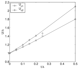
Figure 7: Phase diagram of the ionic Hubbard model. The critical values at $t/\Delta=0.05$ and $0.25$ are taken from Ref. [manma, ].

The values obtained by Manmana et al.manma for $U_{\rm c1}$ and the bounds for $U_{\rm c2}$ from their study of the gaps are also shown in the figure. They fit very nicely on the curves obtained from the peaks of the two-site entropy.

A hint about the nature of the phases can be obtained when the alternation of the two-site entropy $D_{s}$ is looked at. As seen in the third panel of Fig. 6 it vanishes for small and large values of $U/\Delta$ and is finite in the intermediate region only, indicating that in the BO phase, the system is spontaneously dimerized, while it is regular in the BI and MI phases. The critical value where dimerization first appears coincides well with $U_{\rm c1}$, while it cannot be established with certainty that the dimer order disappears exactly at $U_{\rm c2}$, since convergence at the BKT transition is very slow. There is no doubt, however, that the dimer order disappears at large $U$ values and a consistent picture is obtained if it is assumed that spontaneous dimerization occurs in a narrow range only, between the two transitions.

Furthermore, the phase boundaries allow to determine the range where the truncated Hamiltonian can be justified. That is the regime where $(U/\Delta)_{\rm c1}$ and $(U/\Delta)_{\rm c2}$ vary linearly with $t/\Delta$, i.e., where the relevant parameter is the combination $\varepsilon/t\equiv(U-\Delta)/t$. The slopes of the curves give

$$(\varepsilon/t)_{\rm c1}\approx 1.4\,,\qquad(\varepsilon/t)_{\rm c2}\approx 2\,,$$ (25)

and the curvature is rather small up to $t/\Delta\approx 0.5$.

As a check of these results we have repeated the calculations on the unified model at $V=0$ for $\varepsilon>0$. The results for various finite chain lengths are shown in Fig. 8.

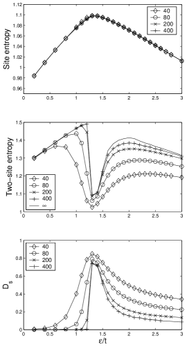
Figure 8: Same as Fig. 6 but for the effective spin-1 model at $V=0$ as a function of $\varepsilon/t\equiv(U-\Delta)/t$.

The site entropy is a rather smooth curve, like for the full model. Even if eventually it develops a cusp at $(\varepsilon/t)_{\rm c1}\simeq 1.3$, there is no indication in the single-site entropy of the second, BKT-like transition. In contrast to this, the two-site entropy exhibits again two maxima. Although for the longest chains the entropy curves have been smoothened close to the maxima due to the fact that the number of block states selected dynamically has reached the maximum number of block states that our code could handle, nevertheless finite-size scaling analysis of the curves gave $(\varepsilon/t)_{\rm c1}\approx 1.3$ and $(\varepsilon/t)_{\rm c2}\approx 2$ for the two critical values, in agreement with our result given in Eq. (25) and with earlier results on the full ionic Hubbard model.legeza ; leo

Moreover, the two-site entropy $D_{s}$ shows clearly that the system is spontaneously dimerized above the first critical value $(\varepsilon/t)_{\rm c1}$, but again although $D_{s}$ certainly vanishes at large enough $\varepsilon/t$, the exact location where this happens cannot be determined from the available chain lengths using finite-size scaling analysis.

IV.2 Large negative values of $\varepsilon/t$

The donor-acceptor model corresponds to $\varepsilon<0$. In the absence of charge transfer between neighbors $(t=0)$ the transition from the neutral to the ionic phase takes place at

$$V={\textstyle\frac{1}{2}}(I-A)\equiv-{\textstyle\frac{1}{2}}\varepsilon\,.$$ (26)

This is a first-order transition where the ionicity jumps from zero to one and none of the gaps go to zero continuously as discussed in Ref. [horovitz, ]. In the neutral state, all sites are in a pure state, the single-site and two-site entropies are zero. In the ionic phase the high degeneracy is due to the arbitrary orientation of the spins, and the site entropy is $\ln 2$, the two-site entropy is $\ln 4$. The jump occurs at the transition point.

For finite $t$ the ionicity and the single-site and two-site entropies are nonvanishing in the neutral phase and their value is less than the maximal one in the ionic phase. Nevertheless, when $t$ is small enough compared to $V$ and $|\varepsilon|$, a finite jump can be detected in these quantities near $V\approx-\varepsilon/2$. The behavior of these quantities as a function of $V/t$ for $\varepsilon/t=-10$ is shown in Fig. 9.

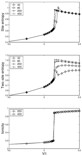
Figure 9: The single-site entropy ($s_{i}$), two-site entropy ($s_{i,i+1}$), and ionicity ($\varrho_{i}$) in the middle of the chains for different chain lengths at $\varepsilon/t=-10$ as a function of $V/t$.

The excitation energies obtained on finite chains using PBC for $\varepsilon/t=-10$ as a function of $V/t$ in the vicinity of the N-I transition are shown in Fig. 10. Although the charge gap $\Delta E_{\rm c}$ has a minimum for all finite $N$, it remains finite even in the thermodynamic limit. The minimum in the $N\rightarrow\infty$ limit is at $V/t\simeq 5.13$, the same value where the ionicity and the entropies have a jump. At the same point, the spin gap $\Delta E_{\rm s}$ and the charge-transfer gap $\Delta E_{\rm CT}$ jump to zero and remain zero for larger $V/t$ values.

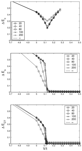
Figure 10: Charge gap, spin gap and charge-transfer gap for a small nonvanishing charge-transfer integral $(\varepsilon/t=-10)$ using PBC.

The dimer order parameter was found to be of the order of $10^{-3}$ or less for all $V/t$ for $N=400$ lattice sites already. Finite-size scaling extrapolation gives less than $10^{-4}$ for the dimer order parameter.

Similar results have been found everywhere for $\varepsilon/t<-8$ except that the transition point shifts to larger $V/t$ values with decreasing $\varepsilon/t$ as expected. We can, therefore, conclude—in agreement with earlier works girlando ; horovitz —that for small values of $t/V$, or equivalently for large negative values of $\varepsilon/t$ the system undergoes a first-order transition from a regular neutral to a regular ionic phase.

IV.3 Smaller values of $\varepsilon/t$

As we have seen, the unified model describes on the one hand the two transitions taking place at $V=0$ and $\varepsilon/t>0$, and on the other hand, the unique first-order transition at large negative values of $\varepsilon/t$. The question we want to address now is how these two limits can be incorporated into a unified phase diagram. We have, therefore, done similar calculations for fixed smaller negative and positive values of $\varepsilon/t$ as a function of $V/t$. The excitation energies obtained on finite chains using OBC for $\varepsilon/t=-2$ are shown in Fig. 11.

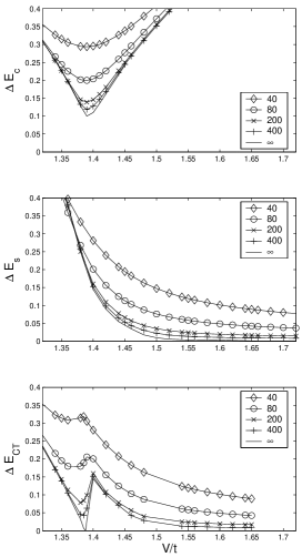
Figure 11: Charge gap, spin gap and charge-transfer gap for $\varepsilon/t=-2$.

Comparison to the results obtained in Ref. [manma, ] shows that the gaps behave surprisingly similarly to that found in the full ionic Hubbard model. The charge-transfer gap vanishes at a critical value $(V/t)_{\rm c1}$ which for $\epsilon/t=-2$ is $(V/t)_{\rm c1}\approx 1.39$, but reopens again and closes a second time at another critical point, whose exact location, however, cannot be determined by finite-size scaling from the available chain lengths. When the same calculations are performed with PBC, the charge-transfer gap vanishes at $(V/t)_{\rm c1}$ and remains zero. Thus the reopening of the gap is due to our use of OBC. As we will see, the system is spontaneously dimerized for $V/t$ larger than this critical value, and as has been discussed in Sec. III, this gives rise to the finite gap between the two lowest lying levels.

The extrapolated spin gap, on the other hand, is finite at $(V/t)_{\rm c1}$ and closes at a second critical value $(V/t)_{\rm c2}$. Due to the very slow decay of the spin gap even on rather long chains, the exact location of the second phase transition could not be determined accurately from the gap.

The charge gap $\Delta E_{\rm c}$ has a minimum for all $N$ and the location of the minimum scales in the thermodynamic limit to $(V/t)_{c1}\simeq 1.39$, however, the gap remains finite at this transition point. The same behavior has been found for the one-particle gap $\Delta_{1}$ in Ref. [manma, ].

The ionicity (not shown) is no longer a good indicator of the neutral-ionic transition, it is found to be a continuous function of $V/t$. Instead of that the dimer order has to be studied, as has been done in the ionic Hubbard model. The behavior is again very similar. The extrapolated value of the measured dimer order parameter is exceedingly small, of the order of $10^{-5}-10^{-4}$ for $V/t<(V/t)_{\rm c1}$. It becomes finite above this transition point, but disappears again at a larger value of $V/t$. Calculations on very long chains ($N=800$) still do not allow a reliable extrapolation to determine the coupling where this happens.

Since it is difficult to locate the second transition from the vanishing of the spin gap or the dimerization, we have studied the behavior of the entropy. Our results obtained on finite chains are shown in Fig. 12.

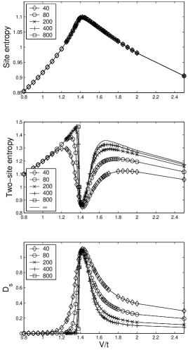
Figure 12: The single-site entropy, two-site entropy, and the dimerization of the two-site entropy for $\varepsilon/t=-2$.

The single-site entropy seems to develop a cusp indicating a second-order phase transition taking place at $(V/t)_{\rm c1}\simeq 1.4$, but only one transition is found. In contrast to this the two-site entropy possesses two maxima for all finite chain lengths and they both develop into a cusp-like peak in the thermodynamic limit. The critical points are at $V/t\simeq 1.39$ and $1.66$. Calculations in the vicinity of $V/t=1.39$ on chains up to $N=800$ lattice sites confirm that although the rise in the two-site entropy is rather steep, there is no jump in it, the transition is of second order.

Similar results, two transitions have been found for other values of $\varepsilon/t$ as a function of $V/t$, when $\varepsilon/t$ is larger than about $-8$. When $\varepsilon/t$ is larger than the critical $(\varepsilon/t)_{\rm c1}\approx 1.3$ or $(\varepsilon/t)_{\rm c2}\approx 2$, one or both transitions appear for negative $V/t$ values.

IV.4 Phase diagram

The results obtained until now can be summarized in the phase diagram shown in Fig. 13.

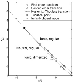
Figure 13: Phase diagram of the unified model describing the ionic Hubbard and donor-acceptor models as a function of the parameters ${\varepsilon/}t$ and $V/t$. Dashed line indicates first-order transition, solid lines correspond to second-order or BKT transitions. The star denotes the tricritical point. The phase boundaries of the full ionic Hubbard model are also shown.

The two transitions obtained in the ionic Hubbard model and the first-order transition of the donor-acceptor model appear in fact as two limiting cases of the unified model. When $\varepsilon$ is negative and $|\varepsilon|\gg t$, the neutral-ionic transition is discontinuous, the ionicity jumps by a finite amount. A tricritical point appears at about $-\varepsilon/t\approx 8$ and $V/t\approx 4.2$, beyond which two transitions are found. The charge-transfer gap vanishes at one of the transitions, while the spin gap does so at the other one.

Since the dimer order parameter is nonvanishing in the narrow region only, between the two continuous transitions, three phases can be identified, a regular neutral, a regular ionic, and a dimerized phase inbetween.

V Conclusion

In summary, we have studied the neutral-ionic transition in organic mixed-stack compounds using the density-matrix renormalization-group method. First, we have shown that a unified model can be derived which is identical to the donor-acceptor model when the intramolecular Coulomb repulsion is the largest energy in the problem and it represents a good approximation to the ionic Hubbard model when $\Delta/t\gg 1$.

Detailed numerical calculations have been performed on this unified model calculating excitation gaps, ionicity, lattice site entropy and dimer order parameter on long chains. We have shown that the best quantity to study is the two-site entropy. It exhibits the transitions most clearly, even at points where finite-size effects are important and the vanishing of gaps in the thermodynamic limit is difficult to establish. In this way we could determine the unified phase diagram as a function of intersite Coulomb interaction and the intraatomic energies. The results are in complete agreement with earlier results on the ionic Hubbard model, while earlier works on the donor-acceptor model have found a single (first or second order) transition only. This is probably due to the closeness of the two transitions, which could not be resolved on short chains.

In the model studied, spontaneous dimerization appears in a narrow range of couplings only, while experiments indicate that the ionic phase is dimerized when electron-phonon coupling is taken into account and the displacement of ions is permitted. Extension of the calculations in this direction is in progress.

- (1) J. B. Torrance, J. E. Vazquez, J. J. Mayerle, and V. Y. Lee, Phys. Rev. Lett. 46, 253 (1981).
- (2) J. B. Torrance, A. Girlando, J. J. Mayerle, J. C. Crowley, V. Y. Lee, P. Batail, and S. J. LaPlaca, Phys. Rev. Lett. 47, 1747 (1981).
- (3) J. Hubbard and J. B. Torrance, Phys. Rev. Lett 47, 1750 (1981).
- (4) M. Fabrizio, A. O. Gogolin, and A. A. Nersesyan, Phys. Rev. Lett. 83, 2014 (1999); Nucl. Phys. B 580, 647 (2000).
- (5) M. E. Torio, A. A. Aligia, and H. C. Ceccatto, Phys. Rev. B 64, 121105(R) (2001).
- (6) Y. Z. Zhang, C. Q. Wu, and H. Q. Lin, Phys. Rev. B 67, 205109 (2003).
- (7) A. P. Kampf, M. Sekania, G. I. Japaridze, and P. Brune, J. Phys.: Condens. Matter 15, 5895 (2003).
- (8) S. R. Manmana, V. Meden, R. M. Noack, and K. Schönhammer, Phys. Rev. B 70, 155115 (2004).
- (9) Z. G. Soos, S. A. Bewick, A. Peri, and A. Painelli, J. Chem. Phys. 120, 6712 (2004).
- (10) A. A. Aligia and C. D. Batista, cond-mat/0412026 (2004).
- (11) L. Tincani, R. Noack and D. Baeriswyl (unpublished).
- (12) Ö. Legeza and J. Sólyom, submitted for publication.
- (13) R. Bruinsmaa, P. Bak, and J. B. Torrance, Phys. Rev. B 27, 456 (1983).
- (14) M. Avignon, C. A. Balseiro, C R. Proetto, and B. Alascio, Phys. Rev. B 33, 205 (1986).
- (15) A. Girlando and A. Painelli, Phys. Rev. B 34, 2131 (1986); A. Painelli and A. Girlando, ibid. 37, 5748 (1988).
- (16) B. Horovitz and J. Sólyom, Phys. Rev. B 35, 7081 (1987).
- (17) Z. G. Soos and S. Mazumdar, Phys. Rev. B 18, 1991 (1978).
- (18) S. R. White, Phys. Rev. Lett. 69, 2863 (1992); Phys. Rev. B 48, 10345 (1993).
- (19) J. Vidal, G. Palacios, R. Mosseri, Phys. Rev. A 69, 022107 (2004); J. Vidal, R. Mosseri, J. Dukelsky, ibid. 69, 054101 (2004).
- (20) Ö. Legeza, J. Röder, and B. A. Hess, Phys. Rev. B 67, 125114 (2003).
- (21) Ö. Legeza and J. Sólyom, Phys. Rev. B 70, 205118 (2004).
- (22) S. R. White, Phys. Rev. Lett. 77, 3633 (1996).
- (23) K. Buchta, G. Fáth, Ö. Legeza and J. Sólyom, Phys. Rev. B 72, 054433 (2005).