Spectral moment sum rules for strongly correlated electrons in time-dependent electric fields

Abstract

We derive exact operator average expressions for the first two spectral moments of nonequilibrium Green’s functions for the Falicov-Kimball model and the Hubbard model in the presence of a spatially uniform, time-dependent electric field. The moments are similar to the well-known moments in equilibrium, but we extend those results to systems in arbitrary time-dependent electric fields. Moment sum rules can be employed to estimate the accuracy of numerical calculations; we compare our theoretical results to numerical calculations for the nonequilibrium dynamical mean-field theory solution of the Falicov-Kimball model at half-filling.

I Introduction

The problem of strong electron correlation is one of the most challenging problems in condensed matter physics. It is interesting because many materials with important properties for applications derive those properties from the delicate balance between minimizing the kinetic and the potential energies in strongly correlated materials. Most theoretical work on this problem has focused on equilibrium properties and linear response, with only limited work available on the nonequilibrium system (which is most easily attained when driven by an external electric field). Two commonly studied models of strong electron correlation are the Hubbard modelHubbard and the Falicov-Kimball modelFalicovKimball (equivalent to the Hubbard model with zero hopping parameter for the down spin electrons). Despite tremendous efforts, the exact equilibrium solution of these models is known only in some limiting cases like one dimension, where the Bethe anzatz techniqueLiebWu can be successfully applied to the Hubbard model, and in the infinite-dimensional case where both models can be solvedGeorges ; Freericks with dynamical mean-field theory (DMFT).

Since the exact solution of these problems is challenging to attain, exact results in the form of sum rules can be quite valuable in determining the fidelity of different approximation techniques (be they analytic, variational, perturbative, or numerical approximations). This problem was analyzed in equilibrium for the Hubbard model by Steve Whitewhite and used to check the accuracy of a quantum Monte Carlo solution to the two-dimensional Hubbard model.

Can similar results be found for nonequilibrium situations, like the case of a strongly correlated material in an uniform external electric field (with arbitrary time dependence)? The answer to this question has, surprisingly, not been discussed much in the literature. It is well known that the canonical anticommutation relation for fermion creation and annihilation operators leads to the integral of the spectral function being 1 in both equilibrium and nonequilibrium situations. It is also well known that the conventional proof that the spectral function is nonnegative in equilibrium (arising from a Lehmann representation), does not apply to the nonequilibrium case, so the spectral function can be negative. It is also known that in the limit of a steady state, the spectral function recovers its nonnegativity. In this work, we examine the theoretical problem of the first few moments of the spectral functions in the presence of an external electric field. It turns out that the equilibrium results for the first few moments are quite similar to the nonequilibrium results, implying they can be used effectively to determine the accuracy of different approximation techniques in solving nonequilibrium problems.

Dynamical mean-field theory has been employed to solve many of the models of strongly correlated electrons. To date, most of this work has focused on equilibrium properties. Schmidt and MonienSchmidtMonien , made a first attempt to solve nonequilibrium DMFT via second-order perturbation theory for the Hubbard model. Their theoretical formulation evaluated the case of a spatially uniform, but time dependent scalar potential, which unfortunately does not correspond to any electric field. More recently, a generalization of the Brandt-Urbanek solutionbrandt_urbanek for the localized electron spectral function allows for an exact numerical solution of the nonequilibrium problem for the Falicov-Kimball modelNashville within the DMFT framework. The procedure works directly in time by discretizing the continuous matrix operators and solving the nonlinear equations by iterating matrix operations on the discretized operators. The approach has been tested against the equilibrium solutionNashville , and nonequilibrium results for the quenching of Bloch oscillations will be presented elsewhere.

In this contribution, we derive operator identities for the first two spectral moments of the nonequilibrium Green’s functions when the strongly correlated material is in the presence of a spatially uniform electric field with arbitrary time dependence. These identities are found for both the Falicov-Kimball and the Hubbard model. Our results are valid for any spatial dimensionality. In the general case, the moments depend on time, which is expected because the field can be turned on at any time; surprisingly, the first two moments of the local retarded Green’s function are time independent, and have the same form as in equilibrium. This last result is particularly surprising because the local retarded Green’s function is a nontrivial oscillating function of time in the noninteracting caseTurkowski .

The rest of the paper is organized as follows. We derive analytical expressions for the spectral moments for the Falicov-Kimball model and the Hubbard model in Section II. The application of nonequilibrium DMFT to the Falicov-Kimball model follows in Section III. Section IV contains results for the Green’s functions and spectral moments in this case. A summary of our results and our conclusions appear in Section V.

II Formalism for the spectral moments

We begin our formal developments with a derivation of exact expressions for the zeroth, first and second spectral moments of the retarded and lesser Green’s functions; the analysis is performed for the spinless Falicov-Kimball model and the spin one-half Hubbard model in an external arbitrary time-dependent spatially uniform electric field. The Hamiltonian for both models has the following form (in the absense of an external field):

$${\mathcal{H}}(0) = -\sum_{ij}t_{ij}c_{i}^{\dagger}c_{j}-\sum_{ij}t_{ij}^{f}f_{i}^{\dagger}f_{j}-\mu\sum_{i}c_{i}^{\dagger}c_{i}$$ (1)

$$- \mu_{f}\sum_{i}f_{i}^{\dagger}f_{i}+U\sum_{i}f_{i}^{\dagger}f_{i}c_{i}^{\dagger}c_{i}.$$

In the case of the Falicov-Kimball model,FalicovKimball  the Hamiltonian in Eq. (1) describes a system which consists of two kinds of spinless electrons: itinerant $c$-electrons with a nearest neighbor hopping matrix $t_{ij}$ and localized $f$-electrons with a hopping matrix equal to zero ($t_{ij}^{f}=0$). We normally take the hopping matrix to be between nearest neighbors only, but this is not a requirement. We do assume the matrix elements are all real and that the hopping matrices are Hermitian. The on-site interaction between the two electrons is equal to $U$. Double occupation by a $c$ or $f$ electron is forbidden by the Pauli exclusion principle. The chemical potentials are $\mu$ and $\mu_{f}$ for the $c$- and $f$-electrons, respectively. We will set $\mu_{f}=0$ in our calculations; it plays no role in the spectral moments of the $c$ particles, which we will be evaluating in this contribution. The spectral moments of the $f$-electrons in equilibrium were worked out in Ref. f_spectral, . In the case of the Hubbard model,Hubbard  the Hamiltonian in Eq. (1) describes a system of spin-up $c\equiv c_{\uparrow}$-electrons, and spin-down $f\equiv c_{\downarrow}$-electrons with equal hopping matrix elements $t_{ij}=t_{ij}^{f}$ and chemical potentials $\mu=\mu_{f}$. The local Coulomb repulsion between electrons with different spins is $U$.

The electric field ${\bf E}({\bf r},t)$ can be described by a vector potential ${\bf A}({\bf r},t)$ in the Hamiltonian or temporal gauge (where the scalar potential vanishes):

$${\bf E}({\bf r},t)=-\frac{1}{c}\frac{\partial{\bf A}({\bf r},t)}{\partial t}$$ (2)

We assume that vector potential ${\bf A}({\bf r},t)$ is smooth enough, that the magnetic field produced by ${\bf A}({\bf r},t)$ can be neglected. For simplicity we shall assume that the vector potential is spatially uniform (independent of r). Note that if we have any time dependence to the electric field, then neglecting the magnetic field will violate Maxwell’s equations. In most situations these magnetic field effects are small enough that they can be neglected in a first analysis, and added back later via either perturbative or gradient-based approaches. The electric field is coupled to the electrons via the Peierls substitution,Jauho  which involves modifying the hopping matrix elements by a phase that depends on the line integral of the vector potential:

$$t_{ij} \rightarrow t_{ij}\exp\left[-\frac{ie}{\hbar c}\int_{{\bf R}_{i}}^{{\bf R}_{j}}{\bf A}({\bf r},t)d{\bf r}\right]$$ (3)

$$= t_{ij}\exp\left[-\frac{ie{\bf A}(t)}{\hbar c}\cdot({\bf R}_{i}-{\bf R}_{j})\right],$$

$$t_{ij}^{f} \rightarrow t_{ij}^{f}\exp\left[-\frac{ie}{\hbar c}\int_{{\bf R}_{i}}^{{\bf R}_{j}}{\bf A}({\bf r},t)d{\bf r}\right]$$ (4)

$$= t_{ij}^{f}\exp\left[-\frac{ie{\bf A}(t)}{\hbar c}\cdot({\bf R}_{i}-{\bf R}_{j})\right].$$

The second line in each equation follows for spatially uniform vector potentials. Note that the Hamiltonian in a field, $\mathcal{H}({\bf A})$, is identical in form to that shown in Eq. (1), but it uses the hopping matrices in Eqs. (3) and (4). Note also that $t^{f}=0$ for the Falicov-Kimball model.

The “Peierls substituted” Hamiltonian in Eq. (1), with the hopping matrix elements in Eqs. (3) and (4), has a simple form in the momentum representation:

$$\mathcal{H}({\bf A}) = \sum_{{\bf k}}\left[\epsilon\left({\bf k}-\frac{e{\bf A}(t)}{\hbar c}\right)-\mu\right]c_{{\bf k}}^{\dagger}c_{{\bf k}}$$ (5)

$$+ \sum_{{\bf k}}\left[\epsilon^{f}\left({\bf k}-\frac{e{\bf A}(t)}{\hbar c}\right)-\mu_{f}\right]f_{{\bf k}}^{\dagger}f_{{\bf k}}$$

$$+ U\sum_{{\bf p},{\bf k},{\bf q}}f_{{\bf p}+{\bf q}}^{\dagger}c_{{\bf k}-{\bf q}}^{\dagger}c_{{\bf k}}f_{{\bf p}},$$

where the fermionic creation and annihilation operators now create or annihilate electrons with well-defined momentum. The free electron energy spectra in Eq. (5) satisfy

$$\epsilon\left({\bf k}-\frac{e{\bf A}(t)}{\hbar c}\right) = \epsilon^{f}\left({\bf k}-\frac{e{\bf A}(t)}{\hbar c}\right)$$

$$= -2t\lim_{d\rightarrow\infty}\sum_{j=1}^{d}\cos\left[a\left({\bf k}_{j}-\frac{e{\bf A}_{j}(t)}{\hbar c}\right)\right],$$

for the Hubbard model. In the case of the Falicov-Kimball model, the $\epsilon^{f}$ term vanishes.

We shall consider the spectral moments for the retarded

$$G_{\bf k}^{R}(t_{1},t_{2})=-i\theta(t_{1}-t_{2})\left\langle\left\{c_{{\bf k}}(t_{1}),c_{{\bf k}}^{\dagger}(t_{2})\right\}\right\rangle$$ (7)

and the lesser

$$G_{\bf k}^{<}(t_{1},t_{2})=i\left\langle c_{{\bf k}}^{\dagger}(t_{2})c_{{\bf k}}(t_{1})\right\rangle$$ (8)

Green’s functions; the symbol $\{O_{1},O_{2}\}=O_{1}O_{2}+O_{2}O_{1}$ is the anticommutator and the operators $c_{{\bf k}}^{\dagger}(t)$ and $c_{{\bf k}}(t)$ are in the Heisenberg representation, where all time dependence is carried by the operators and the states are time-independent. Any Heisenberg representation operator $O_{H}$ is connected with a corresponding Schrödinger representation operator $O_{S}$ via

$$O_{H}(t)=\left[{\mathcal{\bar{T}}}\exp\left\{(i/\hbar)\int_{t_{0}}^{t}d{\bar{t}}\mathcal{H}_{I}({\bar{t}})\right\}\right]e^{(i/\hbar)\mathcal{H}(0)(t-t_{0})}O_{S}$$

$$\times e^{-(i/\hbar)\mathcal{H}(0)(t-t_{0})}\left[\mathcal{T}\exp\left\{-(i/\hbar)\int_{t_{0}}^{t}d{\bar{t}}\mathcal{H}_{I}({\bar{t}})\right\}\right],$$ (9)

where $\mathcal{H}(0)$ is the time-independent part of the Hamiltonian [in Eq. (1) with hopping matrix elements given by their field-free constant values], and $\mathcal{H}_{I}(t)$ is the time-dependent part of the Hamiltonian, which includes the interaction with an external field [but expressed in the interaction representation as detailed in Eq. (10) below]: that is, we define the time-dependent piece in the Schrödinger representation via $\mathcal{H}_{IS}(t)=\mathcal{H}({\bf A})-\mathcal{H}(0)$ and then re-express in the interaction representation. Note that the interaction representation operator is defined to be the Schrödinger representation operator evolved under the time-independent Hamiltonian [i.e., the middle three terms in Eq. (9)]. Hence, the time-dependent piece of the Hamiltonian in the interaction representation is expressed by

$$\mathcal{H}_{I}(t)=e^{(i/\hbar)\mathcal{H}(0)(t-t_{0})}\mathcal{H}_{IS}(t)e^{-(i/\hbar)\mathcal{H}(0)(t-t_{0})},$$ (10)

in terms of the Schrödinger operator; in this form, there is the bare time dependence arising from the time dependence of the fields, plus the time dependence inherited by the operators, as we go from the Schrödinger representation to the interaction representation. The symbol $\mathcal{T}$ ($\mathcal{\bar{T}}$) in Eq. (9) is the time-ordering (anti-time-ordering) operator.

We prepare our system to be in equilibrium prior to the field being turned on, hence the quantum statistical averages in Eqs. (7) and (8) are defined with respect to the zero-field (equilibrium) Hamiltonian $\mathcal{H}(0)$:

$$\langle(...)\rangle={\rm Tr}\left[e^{-\beta\mathcal{H}(0)}(...)\right]/\mathcal{Z},$$ (11)

where the partition function satisfies

$$\mathcal{Z}={\rm Tr}\left[e^{-\beta\mathcal{H}(0)}\right],$$ (12)

and $\beta$ is the inverse temperature of the original equilibrium distribution. As was already mentioned in Section I, the retarded and the lesser Green’s functions form an independent Green’s function basis. Any other Green’s function can be expressed in terms of these two functions. This is in contrast to the equilibrium case, where only one Green’s function is independent (because the Fermi-Dirac distribution function is determined by the equilibrium condition).

Calculations in the nonequilibrium case are complicated by the fact that the Green’s functions in Eqs. (7) and (8) are functions of two time variables, contrary to the equilibrium case, where they only depend on the relative time difference (because the equilibrium system is time-translation invariant). It is convenient to transform the two-time dependence of the Green’s functions from $t_{1}$ and $t_{2}$ to Wigner coordinates, which use the average time $T=(t_{1}+t_{2})/2$ and the relative time $t=t_{1}-t_{2}$ (do not confuse the average time $T$ with the temperature $1/\beta$). Next, the relative time dependence is Fourier transformed to a frequency, and the additional (average) time evolution of different quantities is described by the average time coordinate $T$; in equilibrium, there is no $T$ dependence. For example, the spectral function for the retarded and the lesser Green’s functions can be defined as

$$A_{{\bf k}}^{R,<}(T,\omega)=\int_{-\infty}^{\infty}dte^{i\omega t}\left(\eta\frac{1}{\pi}\right){\rm Im}G_{{\bf k}}^{R,<}(T,t),$$ (13)

where $G_{{\bf k}}^{R,<}(T,t)$ is the respective Green’s function from Eq. (7) or (8) with $t_{1}=T+t/2$ and $t_{2}=T-t/2$; $\eta$ is equal to $-1$ for the retarded Green’s function and $+1$ for the lesser Green’s function so that the spectral functions are nonnegative in equilibrium. In general, the spectral function depends on the average time, because the system no longer has time-translation invariance when a field is turned on at a specific time.

We define the $n$th moment of the retarded and lesser spectral function [in Eq. (13)] $\mu_{n}^{R,<}$ to be

$$\mu_{n}^{R,<}({\bf k},T) = \int_{-\infty}^{\infty}d\omega\omega^{n}A_{{\bf k}}^{R,<}(T,\omega)$$ (14)

$$= \int_{-\infty}^{\infty}d\omega\omega^{n}\left(\eta\frac{1}{\pi}\right){\rm Im}G_{{\bf k}}^{R,<}(T,\omega)$$

$$= \int_{-\infty}^{\infty}d\omega\omega^{n}\left(\eta\frac{1}{\pi}\right)$$

$$\times{\rm Im}\int_{-\infty}^{\infty}dte^{i\omega t}G_{{\bf k}}^{R,<}(T,t).$$

It is easy to show that this expression is equivalent to

$$\mu_{n}^{R,<}({\bf k},T) = \eta\frac{1}{\pi}\int_{-\infty}^{\infty}d\omega$$ (15)

$$\times{\rm Im}\int_{-\infty}^{\infty}dte^{i\omega t}i^{n}\frac{\partial^{n}}{\partial t^{n}}G_{{\bf k}}^{R,<}(T,t).$$

Begin by noting that

$$\frac{\partial^{n}}{(-i)^{n}\partial t^{n}}G_{{\bf k}}^{R,<}(T,t)=\int_{-\infty}^{\infty}\frac{d\omega}{2\pi}e^{-i\omega t}\omega^{n}G_{{\bf k}}^{R,<}(T,\omega),$$ (16)

so that

$$\omega^{n}G_{{\bf k}}^{R,<}(T,\omega)=\int_{-\infty}^{\infty}dte^{i\omega t}\frac{\partial^{n}}{(-i)^{n}\partial t^{n}}G_{{\bf k}}^{R,<}(T,t).$$ (17)

Substituting Eq. (17) into the first line of Eq. (14) then yields Eq. (15). Before proceeding with the evaluation of analytical expressions for the spectral moments from Eq. (15), we note that the integration over frequency in Eq. (15) can be evaluated, yielding the following expression, which connects the spectral moments to the derivative of the Green’s function with respect to relative time $t$ at zero relative time:

$$\mu_{n}^{R,<}({\bf k},T)=\eta 2{\rm Im}\left[i^{n}\frac{\partial^{n}}{\partial t^{n}}G_{{\bf k}}^{R,<}(T,t)\right]_{t=0^{+}}.$$ (18)

This formula assumes that the Green’s function is a differentiable function, which is true in most cases of interest. Despite the fact that the expressions in Eqs. (15) and (18) are formally equivalent, it is preferable to use one or the other in specific cases.

In the case of the retarded Green’s function, the well-known expression for the zeroth spectral moment can be found from Eqs. (18) and (7):

$$\mu_{0}^{R}({\bf k},T)=-2{\rm Im}\left[G_{{\bf k}}^{R}(T,t)\right]_{t=0^{+}}$$ (19)

$$= -2{\rm Im}\left[-i\theta(t)\left\langle\left\{c_{{\bf k}}\left(T+\frac{t}{2}\right),c_{{\bf k}}^{\dagger}\left(T-\frac{t}{2}\right)\right\}\right\rangle\right]_{t=0^{+}}$$

$$= \left\langle\left\{c_{{\bf k}}(T),c_{{\bf k}}^{\dagger}(T)\right\}\right\rangle=1.$$

In the derivation of Eq. (19), we used the anticommutation relation for Heisenberg operators and the fact that the theta function is equal to $1/2$ when its argument is equal to zero.

It is more convenient to use Eqs. (15) and (7) to evaluate the expression for the first moment of $G^{R}$:

$$\mu_{1}^{R}({\bf k},T)=\left(-\frac{1}{\pi}\right)\int_{-\infty}^{\infty}d\omega{\rm Im}\int_{-\infty}^{\infty}dte^{i\omega t}$$ (20)

$$\times \frac{\partial}{\partial t}\left[\theta(t)\left\langle\left\{c_{{\bf k}}\left(T+\frac{t}{2}\right),c_{{\bf k}}^{\dagger}\left(T-\frac{t}{2}\right)\right\}\right\rangle\right].$$

Taking the time derivative in Eq. (20) gives

$$\mu_{1}^{R}({\bf k},T) = -\frac{1}{\pi}\int_{-\infty}^{\infty}d\omega{\rm Im}\int_{-\infty}^{\infty}dte^{i\omega t}\delta(t)$$ (21)

$$\times \left\langle\left\{c_{{\bf k}}\left(T+\frac{t}{2}\right),c_{{\bf k}}^{\dagger}\left(T-\frac{t}{2}\right)\right\}\right\rangle$$

$$+ \frac{1}{\pi}\int_{-\infty}^{\infty}d\omega{\rm Im}\int_{-\infty}^{\infty}dte^{i\omega t}i\theta(t)$$

$$\times \left[\left\langle\left\{i\frac{\partial}{\partial t}c_{{\bf k}}\left(T+\frac{t}{2}\right),c_{{\bf k}}^{\dagger}\left(T-\frac{t}{2}\right)\right\}\right\rangle\right.$$

$$+ \left.\left\langle\left\{c_{{\bf k}}\left(T+\frac{t}{2}\right),i\frac{\partial}{\partial t}c_{{\bf k}}^{\dagger}\left(T-\frac{t}{2}\right)\right\}\right\rangle\right].$$

The first term in Eq. (21) is equal to zero, because the integral over time is equal to $1$, therefore its imaginary part vanishes. The second term in Eq. (21) can be simplified by performing an integration over $\omega$ and replacing the time derivatives of the operators by their commutators with the Hamiltonian, according to the Heisenberg equation of motion $i\partial O(t)/\partial t\ =[O(t),\mathcal{H}(t)]$, where $\mathcal{H}(t)$ is the total Hamiltonian including the effects of the time-dependent field. This yields

$$\mu_{1}^{R}({\bf k},T) = \frac{1}{2}{\rm Re}\left(\left\langle\left\{[c_{{\bf k}}(T),\mathcal{H}(T)],c_{{\bf k}}^{\dagger}(T)\right\}\right\rangle\right.$$ (22)

$$- \left.\left\langle\left\{c_{{\bf k}}(T),[c_{{\bf k}}^{\dagger}(T),\mathcal{H}(T)]\right\}\right\rangle\right).$$

Evaluation of the commutators of the Fermi-operators with the Hamiltonian and the subsequent anticommutators in Eq. (5) gives the following expression for the first spectral moment of the retarded Green’s function

$$\mu_{1}^{R}({\bf k},T)=\epsilon\left({\bf k}-\frac{e{\bf A}(T)}{\hbar c}\right)-\mu+Un_{f},$$ (23)

where

$$n_{f}=\sum_{{\bf k}}\langle f_{{\bf k}}^{\dagger}(T)f_{{\bf k}}(T)\rangle$$ (24)

is the average number of $f$ ($c_{\downarrow}$)-electrons in the system; this number of electrons does not depend on the average or the relative time, because the total electron number for each species of electron is conserved.

Similarly, the expression for the second moment of the retarded Green’s function can be found from Eqs. (15) and (7):

$$\mu_{2}^{R}({\bf k},T) = \frac{1}{4}{\rm Re}\left(\left\langle\left\{[[c_{{\bf k}}(T),\mathcal{H}(T)],\mathcal{H}(T)],c_{{\bf k}}^{\dagger}(T)\right\}\right\rangle\right.$$ (25)

$$- 2\left\langle\left\{[c_{{\bf k}}(T),\mathcal{H}(T)],[c_{{\bf k}}^{\dagger}(T),\mathcal{H}(T)]\right\}\right\rangle$$

$$+ \left.\left\langle\left\{c_{{\bf k}}(T),[[c_{{\bf k}}^{\dagger}(T),\mathcal{H}(T)],\mathcal{H}(T)]\right\}\right\rangle\right).$$

Details of the derivation are presented in the Appendix.

Evaluating the commutators and anticommutators in Eq. (25) gives

$$\mu_{2}^{R}({\bf k},T) = \left[\epsilon\left({\bf k}-\frac{e{\bf A}(T)}{\hbar c}\right)-\mu\right]^{2}$$

$$+ 2U\left[\epsilon\left({\bf k}-\frac{e{\bf A}(T)}{\hbar c}\right)-\mu\right]n_{f}+U^{2}n_{f}.$$

The moments of the local retarded Green’s function ${\tilde{\mu}}_{n}^{R}(T)$ are obtained by summing the corresponding spectral moment functions $\mu_{n}^{R}({\bf k},T)$ over ${\bf k}$

$${\tilde{\mu}}_{n}^{R}(T)=\sum_{{\bf k}}\mu_{n}^{R}({\bf k},T).$$ (27)

Performing the summations for Eqs. (23) and (II) yields the following local moments:

$${\tilde{\mu}}_{1}^{R}(T) = -\mu+Un_{f};$$ (28)

$${\tilde{\mu}}_{2}^{R}(T) = \frac{1}{2}+\mu^{2}-2U\mu n_{f}+U^{2}n_{f}.$$ (29)

These results coincide with those derived previously for the Hubbard model in the equilibrium casewhite . Since the hopping matrix is always chosen to be traceless in our models, the sum of the energy $\sum_{{\bf k}}\epsilon({\bf k})$ in Eqs. (23) and (II) is equal to zero. The expression for the zeroth local moment ${\tilde{\mu}}_{0}^{R}$ has the same form as the expression for the zeroth spectral moment in Eq. (19), since the zeroth spectral moment is momentum-independent. Hence, the zeroth and the first two local moments of the retarded Green’s function in an arbitrary external time-dependent homogeneous electric field are all time-independent! This is a nontrivial result because the retarded Green’s function strongly depends on the average time. In particular, the retarded Green’s function is an oscillating function of timeTurkowski when $U=0$. Furthermore, the moments do not depend on the electric field at half-filling because the chemical potential is not changed by the field! It isn’t obvious whether the chemical potential would be changed by the field off of half-filling.

In the case of half-filling, where $n_{c}=n_{f}=1/2$ and $\mu=U/2$, the expressions in Eqs. (19), (28) and (29) acquire an even simpler form:

$${\tilde{\mu}}_{0}^{R}(T) = 1,$$ (30)

$${\tilde{\mu}}_{1}^{R}(T) = 0,$$ (31)

$${\tilde{\mu}}_{2}^{R}(T) = \frac{1}{2}+\frac{U^{2}}{4}.$$ (32)

If one examines the moments for gauge-invariant Green’s functions,gauge_inv  then the local moments are unchanged, and the spectral function moments are modified by a time-dependent shift of the momentum wavevector. We don’t include those formulas here, because they just involve such a simple shift.

The corresponding moments of the lesser Green’s functions are found by a similar analysis. Using Eqs. (18) and (8) we find

$$\mu_{0}^{<}({\bf k},T) = 2n_{c}({\bf k},T),$$ (33)

$$\mu_{1}^{<}({\bf k},T) = -{\rm Re}\left(\left\langle[c_{{\bf k}}^{\dagger}(T),\mathcal{H}(T)]c_{{\bf k}}(T)\right\rangle\right.$$ (34)

$$- \left.\left\langle c_{{\bf k}}^{\dagger}(T)[c_{{\bf k}}(T),\mathcal{H}(T)]\right\rangle\right),$$

$$\mu_{2}^{<}({\bf k},T) = \frac{1}{2}{\rm Re}\left(\left\langle[[c_{{\bf k}}^{\dagger}(T),\mathcal{H}(T)],\mathcal{H}(T)]c_{{\bf k}}(T)\right\rangle\right.$$ (35)

$$- \left.2\left\langle[c_{{\bf k}}^{\dagger}(T),\mathcal{H}(T)][c_{{\bf k}}(T),\mathcal{H}(T)]\right\rangle\right.$$

$$+ \left.\left\langle c_{{\bf k}}^{\dagger}(T)[[c_{{\bf k}}^{\dagger}(T),\mathcal{H}(T)],\mathcal{H}(T)]\right\rangle\right),$$

where

$$n_{c}({\bf k},T)=\left\langle c_{{\bf k}}^{\dagger}(T)c_{{\bf k}}(T)\right\rangle$$ (36)

is the momentum distribution function for the $c$ $(c_{\uparrow})$-electrons. Note that a commutator term depending on the derivative of the Hamiltonian with respect to time can be shown to cancel, so it is not included in the second moment expression above. Evaluation of the commutators of the operators with the Hamiltonian [in Eq. (5)] in Eqs. (34) and (35) gives

$$\mu_{1}^{<}({\bf k},T)=2\left[\epsilon\left({\bf k}-\frac{e{\bf A}(T)}{\hbar c}\right)-\mu\right]n_{c}({\bf k},T)$$

$$+U\sum_{{\bf p},{\bf q}}\left(\left\langle f_{{\bf p}+{\bf q}}^{\dagger}c_{{\bf k}-{\bf q}}^{\dagger}c_{{\bf k}}f_{{\bf p}}\right\rangle+\left\langle f_{{\bf p}+{\bf q}}^{\dagger}c_{{\bf k}}^{\dagger}c_{{\bf k}+{\bf q}}f_{{\bf p}}\right\rangle\right).$$ (37)

and

$$\mu_{2}^{<}({\bf k},T) = 2\left[\epsilon\left({\bf k}-\frac{e{\bf A}(T)}{\hbar c}\right)-\mu\right]^{2}n_{c}({\bf k},T)+\frac{3}{2}U\left[\epsilon\left({\bf k}-\frac{e{\bf A}(T)}{\hbar c}\right)-\mu\right]\sum_{{\bf p},{\bf q}}\left(\left\langle f_{{\bf p}+{\bf q}}^{\dagger}c_{{\bf k}-{\bf q}}^{\dagger}c_{{\bf k}}f_{{\bf p}}\right\rangle+\left\langle f_{{\bf p}+{\bf q}}^{\dagger}c_{{\bf k}}^{\dagger}c_{{\bf k}+{\bf q}}f_{{\bf p}}\right\rangle\right)$$

$$+ \frac{1}{2}U\sum_{{\bf p},{\bf q}}\left[\epsilon\left({\bf k}-{\bf q}-\frac{e{\bf A}(T)}{\hbar c}\right)-\mu\right]\left\langle f_{{\bf p}+{\bf q}}^{\dagger}c_{{\bf k}-{\bf q}}^{\dagger}c_{{\bf k}}f_{{\bf p}}\right\rangle+\frac{1}{2}U\sum_{{\bf p},{\bf q}}\left[\epsilon\left({\bf k}+{\bf q}-\frac{e{\bf A}(T)}{\hbar c}\right)-\mu\right]\left\langle f_{{\bf p}+{\bf q}}^{\dagger}c_{{\bf k}}^{\dagger}c_{{\bf k}+{\bf q}}f_{{\bf p}}\right\rangle$$

$$+ \frac{1}{2}U\sum_{{\bf p},{\bf q}}\epsilon^{f}\left({\bf p}+{\bf q}-\frac{e{\bf A}(T)}{\hbar c}\right)\left[\left\langle f_{{\bf p}+{\bf q}}^{\dagger}c_{{\bf k}}^{\dagger}c_{{\bf k}+{\bf q}}f_{{\bf p}}\right\rangle-\left\langle f_{{\bf p}+{\bf q}}^{\dagger}c_{{\bf k}-{\bf q}}^{\dagger}c_{{\bf k}}f_{{\bf p}}\right\rangle\right]$$

$$- \frac{1}{2}U\sum_{{\bf p},{\bf q}}\epsilon^{f}\left({\bf p}-\frac{e{\bf A}(T)}{\hbar c}\right)\left[\left\langle f_{{\bf p}+{\bf q}}^{\dagger}c_{{\bf k}}^{\dagger}c_{{\bf k}+{\bf q}}f_{{\bf p}}\right\rangle-\left\langle f_{{\bf p}+{\bf q}}^{\dagger}c_{{\bf k}-{\bf q}}^{\dagger}c_{{\bf k}}f_{{\bf p}}\right\rangle\right]$$

$$+ \frac{1}{2}U^{2}\sum_{{\bf p},{\bf q},{\bf P},{\bf Q}}\left[\left\langle f_{{\bf p}+{\bf q}}^{\dagger}f_{{\bf p}}f_{{\bf P}+{\bf Q}}^{\dagger}f_{{\bf P}}c_{{\bf k}-{\bf q}-{\bf Q}}^{\dagger}c_{{\bf k}}\right\rangle+2\left\langle f_{{\bf p}+{\bf q}}^{\dagger}f_{{\bf p}}f_{{\bf P}+{\bf Q}}^{\dagger}f_{{\bf P}}c_{{\bf k}-{\bf q}}^{\dagger}c_{{\bf k}+{\bf Q}}\right\rangle\right.$$

$$+ \left.\left\langle f_{{\bf p}+{\bf q}}^{\dagger}f_{{\bf p}}f_{{\bf P}+{\bf Q}}^{\dagger}f_{{\bf P}}c_{{\bf k}}^{\dagger}c_{{\bf k}+{\bf q}+{\bf Q}}\right\rangle\right].$$

In Eq. (II), we have suppressed the time label $T$ corresponding to the time at which all operators are evaluated. We continue to suppress this time label in some equations below; this should not cause any confusion.

The expressions in Eqs. (33)–(II) for the lesser spectral moments are more complicated than the corresponding retarded moments. However, they simplify in the case of the local Green’s function, where we find

$${\tilde{\mu}}_{0}^{<}(T) = 2n_{c},$$ (39)

$${\tilde{\mu}}_{1}^{<}(T) = 2\sum_{{\bf k}}\left[\epsilon\left({\bf k}-\frac{e{\bf A}(T)}{\hbar c}\right)-\mu\right]n_{c}({\bf k},T)$$ (40)

$$+ 2U\sum_{i}\left\langle f_{i}^{\dagger}f_{i}c_{i}^{\dagger}c_{i}\right\rangle,$$

$${\tilde{\mu}}_{2}^{<}(T) = 2\sum_{{\bf k}}\left[\epsilon\left({\bf k}-\frac{e{\bf A}(T)}{\hbar c}\right)-\mu\right]^{2}n_{c}({\bf k},T)$$ (41)

$$+ 2U\sum_{{\bf k},{\bf p},{\bf q}}\left[\epsilon\left({\bf k}-\frac{e{\bf A}(T)}{\hbar c}\right)\right.$$

$$\quad+\left.\epsilon\left({\bf k}-{\bf q}-\frac{e{\bf A}(T)}{\hbar c}\right)\right]\left\langle f_{{\bf p}+{\bf q}}^{\dagger}f_{{\bf p}}c_{{\bf k}-{\bf q}}^{\dagger}c_{{\bf k}}\right\rangle$$

$$- 2U(2\mu-U)\sum_{i}\left\langle f_{i}^{\dagger}f_{i}c_{i}^{\dagger}c_{i}\right\rangle,$$

with

$$n_{c}=\sum_{{\bf k}}n_{c}({\bf k},T)$$ (42)

being the time-independent particle density of the $c$ ($c_{\uparrow}$)-electrons. In order to save space, and make the equations more transparent, we use a mixed real-space/momentum-space representation for the operators in Eqs. (40) and (41). Note that the first moment involves one correlation function and the second moment involves two correlation functions. Note further that the value of the first moment in Eq. (40) is equal to twice the average value of the Hamiltonian. The last term in Eq. (41) is equal to zero in the case of half-filling ($\mu=U/2$). The second two moments of the lesser Green’s functions do appear to depend both on the average time and the electric field (although our empirical evidence at half filling suggests the second moment may be independent of average time—see the numerical results below).

There is an interesting observation that can be made about the first moment, and its relation to the current driven by the electric field and the phenomenon of Bloch oscillations. In the limit where $U$ is small, one can evaluate the correlation function in Eq. (40) via a mean-field theory decoupling ($\langle f_{i}^{\dagger}f_{i}c_{i}^{\dagger}c_{i}\rangle\approx\langle f_{i}^{\dagger}f_{i}\rangle\langle c_{i}^{\dagger}c_{i}\rangle$). For example, at half filling, the first moment will be equal to twice the average kinetic energy (including the shift by the vector potential needed to construct the actual kinetic energy from the bandstructure) plus a correction of order $U^{2}$. If the current oscillates, we expect the average kinetic energy to oscillate as well. Hence, for small $U$ there is a correlation between oscillations in the first moment of the local Green’s function and oscillations of the current.

The correlation function $\left\langle f^{\dagger}_{i}f_{i}c^{\dagger}_{i}c_{i}\right\rangle$ that appears in Eqs. (40) and (41) can be determined for the Falicov-Kimball or Hubbard model via the equation of motion, because it is related to the total energy of the Hamiltonian. To show how this works, we first provide the derivation for the equilibrium case using an imaginary-time formalism. Begin with the definition of the Green’s function in real space

$$G_{ij}(\tau)=-\left\langle\mathcal{T}c_{i}(\tau)c_{j}^{\dagger}(0)\right\rangle,$$ (43)

with a similar result for the spin-down electrons in the Hubbard model. Here we have $c_{i}(\tau)=\exp(\mathcal{H}\tau)c_{i}(0)\exp(-\mathcal{H}\tau)$. Taking the imaginary-time derivative of the local Green’s function gives

$$\partial_{\tau}G_{ii}(\tau) = -\delta(\tau)-\left\langle\mathcal{T}[\mathcal{H},c_{i}(\tau)]c^{\dagger}_{i}(0)\right\rangle$$ (44)

$$= -\delta(\tau)+t\sum_{\delta}G_{i+\delta i}(\tau)+\mu G_{ii}(\tau)$$

$$+ U\left\langle\mathcal{T}f_{i}^{\dagger}f_{i}c_{i}(\tau)c_{i}^{\dagger}(0)\right\rangle,$$

where the symbol $\delta$ denotes the translation vector to a nearest-neighbor site and $i+\delta$ as a subscript refers to the lattice site that is the nearest neighbor of site $i$ translated by the nearest-neighbor translation vector $\delta$. Hence we determine the correlation function via

$$U\left\langle\mathcal{T}f_{i}^{\dagger}f_{i}c_{i}^{\dagger}c_{i}\right\rangle = \lim_{\tau\rightarrow 0^{-}}\left[-\partial_{\tau}G_{ii}(\tau)\right.$$

$$+ \left.t\sum_{\delta}G_{i+\delta i}(\tau)+\mu G_{ii}(\tau)-\delta(\tau)\right].$$

Using the Matsubara frequency representation

$$G(i\omega_{n})=G_{n}=\int_{0}^{\beta}d\tau e^{i\omega_{n}\tau}G(\tau),$$ (46)

with $i\omega_{n}=i\pi(2n+1)/\beta$ the fermionic Matsubara frequency, allows us to determine a simple expression for the correlation function. Note that $G(\tau)=(1/\beta)\sum_{n}\exp(-i\omega_{n}\tau)G_{n}$ and that the Green’s function in momentum space satisfies $G_{n}({\bf k})=1/[i\omega_{n}+\mu-\Sigma_{n}({\bf k})-\epsilon({\bf k})]$, to find that the correlation function simplifies to

$$\left\langle\mathcal{T}f_{i}^{\dagger}f_{i}c_{i}c_{i}^{\dagger}\right\rangle=\frac{1}{\beta U}\sum_{n}\sum_{\bf k}\frac{\Sigma_{n}({\bf k})}{i\omega_{n}+\mu-\Sigma_{n}({\bf k})-\epsilon({\bf k})}.$$ (47)

In the limit of infinite dimensions, the self-energy is a local function, and hence has no momentum dependence. Then the sum over momentum can be performed by changing from a sum over momentum to an integral over the noninteracting density of states. This produces the local Green’s function, and we are left with the final form for DMFT:

$$\left\langle\mathcal{T}f_{i}^{\dagger}f_{i}c_{i}^{\dagger}c_{i}\right\rangle=\frac{1}{\beta U}\sum_{n}\Sigma_{n}G_{n}.$$ (48)

In numerical calculations, it is more convenient to evaluate the summation in Eq. (48) via the formally equivalent expression with the Hartree-Fock contribution to the self-energy removed

$$\left\langle\mathcal{T}f_{i}^{\dagger}f_{i}c_{i}^{\dagger}c_{i}\right\rangle=\langle f^{\dagger}f\rangle\langle c^{\dagger}c\rangle+\frac{1}{\beta U}\sum_{n}[\Sigma_{n}-U\langle f^{\dagger}f\rangle]G_{n},$$ (49)

because the Matsubara summation converges faster.

In the nonequilibrium case, one can perform a similar analysis, but now one has to work with the nonequilibrium Green’s functions as functions of real time variables. Using the standard equations of motion, and definitions for nonequilibrium Green’s functions, one can show, after some significant algebra, that the correlation function can be expressed as

$$U\left\langle f_{i}^{\dagger}f_{i}c_{i}^{\dagger}c_{i}\right\rangle = -i\sum_{\bf k}\left[i\frac{\partial}{\partial t_{1}}+\mu-\epsilon\left({\bf k}-\frac{e{\bf A}(t_{1})}{\hbar c}\right)\right]$$ (50)

$$\times G^{<}_{\bf k}(t_{1},t_{2})\Biggr{|}_{t_{2}=t_{1}}$$

$$= -i\sum_{\bf k}\int dt\left[\Sigma^{R}_{\bf k}(t_{1},t)G^{<}_{\bf k}(t,t_{1})\right.$$

$$+ \left.\Sigma^{<}_{\bf k}(t_{1},t)G^{A}_{\bf k}(t,t_{1})\right],$$

where the final result is written in terms of retarded, lesser and advanced Green’s functions and self-energies in the presence of the field. In the DMFT limit, the self-energies have no momentum dependence. This expression appears like it can have average time dependence, but we cannot say that it definitely does, because there could be a cancellation of the time dependence.

As a check of Eq. (50), we evaluate it in equilibrium, to show it yields the same result as Eq. (48). When we are in equilibrium, the correlation function is independent of time and the Green’s functions and self-energies depend only on the time difference of their two time variables. Hence, we can perform a Fourier transform by using the convolution theorem to transform Eq. (50) into

$$U\left\langle f_{i}^{\dagger}f_{i}c_{i}^{\dagger}c_{i}\right\rangle = -\frac{i}{2\pi}\sum_{\bf k}\int d\omega\left[\Sigma^{R}_{\bf k}(\omega)G^{<}_{\bf k}(\omega)\right.$$ (51)

$$+ \left.\Sigma^{<}_{\bf k}(\omega)G^{A}_{\bf k}(\omega)\right].$$

Using the fact that the lesser functions satisfy $G^{<}_{\bf k}=-2if(\omega){\rm Im}G^{R}_{\bf k}(\omega)$ and $\Sigma^{<}_{\bf k}=-2if(\omega){\rm Im}\Sigma^{R}_{\bf k}(\omega)$ in equilibrium, allows us to transform Eq. (51) into

$$U\left\langle f_{i}^{\dagger}f_{i}c_{i}^{\dagger}c_{i}\right\rangle=-\frac{1}{\pi}\sum_{\bf k}\int d\omega f(\omega){\rm Im}\left[\Sigma_{\bf k}^{R}(\omega)G^{R}_{\bf k}(\omega)\right],$$ (52)

which is equal to the analytic continuation of Eq. (48) from the imaginary axis to the real axis.

The correlation function $\left\langle f_{{\bf p}+{\bf q}}^{\dagger}f_{{\bf p}}c_{{\bf k}-{\bf q}}^{\dagger}c_{{\bf k}}\right\rangle$ which enters Eq. (41) is more complicated to evaluate, because it cannot be expressed in terms of a simple equation of motion for the single-particle Green’s functions. Because of it’s complex nature, we will evaluate it only for the Falicov-Kimball model in equilibrium. While it is certainly true that it can be evaluated for the Falicov-Kimball model in the presence of a field, some of the formal details become quite complicated, and take us away from the main theme of this work, so we do not perform such an analysis here.

Our starting point, then, is the operator average

$$\sum_{\bf k,p,q}\left[\epsilon({\bf k})+\epsilon({\bf k}-{\bf q})\right]\left\langle f_{{\bf p}+{\bf q}}^{\dagger}f_{{\bf p}}c_{{\bf k}-{\bf q}}^{\dagger}c_{{\bf k}}\right\rangle,$$ (53)

where we have set the vector potential ${\bf A}$ equal to zero. We use a Fourier transform to express the localized electrons in terms of their real-space operators. Then Elitzur’s theoremelitzur ensures that the operator expectation value vanishes if the two localized electrons are not at the same lattice site (i.e., there is no spontaneous hybridization in the Falicov-Kimball model for nonzero temperature). This allows us to perform the summation over the momentum variable ${\bf p}$ and gives us

$$\sum_{\bf k,q}\sum_{i}\left[\epsilon({\bf k})+\epsilon({\bf k}-{\bf q})\right]e^{i{\bf q}\cdot{\bf R_{i}}}\left\langle f_{i}^{\dagger}f_{i}c_{{\bf k}-{\bf q}}^{\dagger}c_{{\bf k}}\right\rangle.$$ (54)

Next, we express the bandstructure in terms of the summation over nearest neighbor translation vectors $\delta$: $\epsilon({\bf k})=-t^{*}\sum_{\delta}\exp[i{\bf k}\cdot\delta]/\sqrt{d}$, and introduce Fourier transforms for the itinerant electrons to real space. This allows us to sum over the remaining momenta, yielding

$$-\frac{t^{*}}{\sqrt{d}}\sum_{i\delta}\left[\left\langle f_{i}^{\dagger}f_{i}c_{i}^{\dagger}c_{i+\delta}\right\rangle+\left\langle f_{i}^{\dagger}f_{i}c_{i+\delta}^{\dagger}c_{i}\right\rangle\right].$$ (55)

The statistical averages in Eq. (55) have already been evaluated.thermal  The procedure is to imagine adding a small field $-\sum_{i}h_{i}f^{\dagger}_{i}f_{i}$ to the Hamiltonian, and evaluate the expectation value with the localized particle number via a derivative with respect to the field strength $h_{i}$ (then set the field to zero to evaluate the average). This gives

$$-\frac{t^{*}}{\sqrt{d}}\sum_{i\delta}\left[\frac{1}{\beta}\frac{\partial}{\partial h_{i}}+\langle w_{i}\rangle\right]\left[\left\langle c_{i}^{\dagger}c_{i+\delta}\right\rangle+\left\langle c_{i+\delta}^{\dagger}c_{i}\right\rangle\right]$$ (56)

$$= -\frac{t^{*}}{\sqrt{d}}\sum_{i\delta}\left[\frac{1}{\beta}\frac{\partial}{\partial h_{i}}+\langle w_{i}\rangle\right]$$

$$\times\left[G_{i+\delta i}(\tau\rightarrow 0^{-})+G_{ii+\delta}(\tau\rightarrow 0^{-})\right].$$

Now we follow the derivation in Ref. thermal, , which evaluates the derivatives from the following:

$$\left[\frac{1}{\beta}\frac{\partial}{\partial h_{i}}+\langle w_{i}\rangle\right]G_{i+\delta i}(\tau\rightarrow 0^{-})$$

$$=\frac{1}{\beta}\sum_{n}\sum_{jk}G_{i+\delta j}\left[-\frac{1}{\beta}\frac{\partial}{\partial h_{i}}+\langle w_{i}\rangle\right]G^{-1}_{jk}(i\omega_{n})G_{ki}(i\omega_{n})$$

$$=\frac{1}{\beta}\sum_{n}\left[G_{i+\delta i}\frac{1}{\beta}\frac{\partial}{\partial h}\Sigma(i\omega_{n})G_{ii}(i\omega_{n})+\langle f^{\dagger}f\rangle G_{ii}(i\omega_{n})\right]$$

where the derivative with respect to the field $h$ acts on the local self-energy. After some long and complicated algebra, that derivative can be determined, which yields our final result for the correlation function

$$\frac{2}{\beta}\sum_{n}\sum_{\bf k}\frac{\epsilon({\bf k})}{U}G_{\bf k}(i\omega_{n})\Sigma(i\omega_{n})$$ (58)

$$= \frac{2}{\beta U}\sum_{n}\left[-1+(i\omega_{n}+\mu-\Sigma_{n})G_{n}\right]\Sigma_{n}.$$

This result is quite similar to the previous result for the other correlation function, except now we have an extra weighting factor of $2\epsilon({\bf k})$ in the summation over momentum.

III The Falicov-Kimball model in infinite dimensions

In this Section, we examine the time-dependence of the local Green’s function for the Falicov-Kimball model on an infinite-dimensional hypercubic lattice. We consider the case of half-filling with the system being coupled to an external homogeneous time-dependent electric field. The time dependence is taken to be particularly simple, at $t=t_{0}$ a constant field is instantly turned on. The formalism involves generalizing the DMFT to the nonequilibrium case. The way to do this is based on a Kadanoff-Baym approach in real time, where continuous matrix operators are discretized along the Kadanoff-Baym contour, and operator manipulations are carried out on the discretized matrices using standard linear-algebra approaches. A short description of this technique, including a benchmark against the well-known equilibrium solutions has already appearedNashville ; further details of this approach will appear elsewhere. To test our formulas for the first few moments, we compare numerically calculated local moments to the exact moments in Eqs. (30–32) and (39–41).

The action for the Falicov-Kimball model is quadratic in the conduction electrons. Hence the Feynman path integral over the Kadanoff-Baym contour can be expressed by a determinant of a continuous matrix operator whose arguments are defined on the contour. Since the concentration of static particles on each site is conserved, the trace over the fermionic variables can be straightforwardly taken. This is what allows the nonequilibrium DMFT problem to be solved, but the technical details are complicated. The first thing that needs to be noted is that the self-energy remains local even in the presence of a field. This follows by applying Langreth’s ruleslangreth to the perturbation theory, which state that every nonequilibrium diagram can be related to an equilibrium diagram, but now one must perform the analysis over the Kadanoff-Baym contour rather than over the finite imaginary time interval. Since the perturbative analysis of the equilibrium problem shows the self-energy to be localbrandt_mielsch ; metzner ; Freericks in equilibrium, it remains local in the nonequilibrium case as well.

We couple the system in Eq. (5) to an external electric field along the unit-cell diagonal direction in real space; this yields the following vector potential for the electric fieldTurkowski :

$${\bf A}(t)=A(t)(1,1,...,1).$$ (59)

The bandstructure for noninteracting electrons coupled to the electric field in Eq. (59) has a simple form:

$$\epsilon\left({\bf k}-\frac{e{\bf A}(t)}{\hbar c}\right)=\cos\left(\frac{eaA(t)}{\hbar c}\right)\varepsilon_{\bf k}+\sin\left(\frac{eaA(t)}{\hbar c}\right){\bar{\varepsilon}}_{\bf k},$$ (60)

with the energy functions defined to be

$$\varepsilon_{\bf k}=-\frac{t^{*}}{\sqrt{d}}\sum_{j}\cos(a{\bf k}_{j})$$ (61)

and

$${\bar{\varepsilon}}_{\bf k}=-\frac{t^{*}}{\sqrt{d}}\sum_{j}\sin(a{\bf k}_{j}),$$ (62)

and $t^{*}$ is the renormalized hopping parametermetzner_vollhardt in the limit of $d\rightarrow\infty$; we take $t=t^{*}/2\sqrt{d}$.

Because the Green’s functions now depend on two energies, the summation over the infinite-dimensional Brillouin zone can be replaced by a double integral over a joint density of states for the two energies. This joint density of states (DOS) isSchmidtMonien

$$\rho_{2}(\varepsilon,{\bar{\varepsilon}})=\frac{1}{\pi t^{*2}a^{d}}\exp\left[-\frac{\varepsilon^{2}}{t^{*2}}-\frac{{\bar{\varepsilon}}^{2}}{t^{*2}}\right].$$ (63)

The numerical integration over the joint DOS is performed by an averaged Gaussian integration with 54 and 55 points for each energy axis:

$$\int_{-\infty}^{\infty}d\varepsilon\exp(-\varepsilon^{2})F(\varepsilon)\simeq\sum_{i=1}^{N}w_{i}F(\varepsilon_{i}),$$ (64)

where $w_{i}$ are Gaussian weights which correspond to the $N$ energy points $\varepsilon_{i}$. Since the Green’s functions often depend on the energy as $\exp(ic\varepsilon)$, the Gaussian quadrature rule in Eq. (64) fails to give correct results when $c$ is on the order of (or larger than) the inverse of the grid spacing of the energy points near $\varepsilon=0$. In this case, the sum over discrete points contains a systematic contribution of terms which do not cancel each other, and leads to an overestimated value to the integral. One way to efficiently correct this is to average two Gaussian summations with numbers of Gaussian points equal to $N$ and $N+1$ because the Gaussian points interleave each other, and act like a step size about half as big as either sum alone, and they give somewhat better accuracy than performing the integral with $2N+1$ points, because a subset of those points are at such large absolute value that the Gaussian weight is small enough that it can be safely neglected.

In order to calculate the nonequilibrium local Green’s functions, one needs to self-consistently solve a system of equationsNashville which connects these functions with the corresponding local self-energy $\Sigma(t_{1},t_{2})$ and an effective dynamical mean-field $\lambda(t_{1},t_{2})$; these equations are similar in form to the equilibrium case,Georges ; Freericks  but now all the functions are discrete matrices of two time variables defined on the Kadanoff-Baym contour (see Fig. 1). Details of the algorithm and the nonequilibrium DMFT equations will be given elsewhereunpublished .

Figure 1: Kadanoff-Baym contour for the two-time Green’s functions in the nonequilibrium case. We take the contour to run from $-t_{max}$ to $t_{max}$ and back, and then extends downward parallel to the imaginary axis for a distance of $\beta$. The field is usually turned on at $t=0$; i.e., the vector potential is nonzero only for positive times.

First, we present results for the local moments in equilibrium, when the system of the DMFT equations is solved in the frequency representation using the Brandt-Mielsch approachbrandt_mielsch (for details, see Ref. Freericks, ). Plots of the local retarded and lesser DOS for different values of $U$ are shown in Figs. 2 and 3. The metal-insulator transition occurs at $U=\sqrt{2}$; the insulator has anomalous properties because there is no real gap—instead the DOS is exponentially small in a gap region around the chemical potential, and vanishes only at the chemical potential.

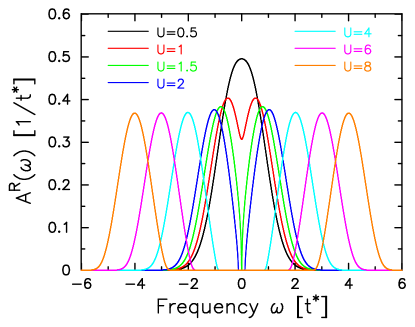
Figure 2: DOS for the equilibrium retarded Green’s function for different values of $U$. The DOS is independent of temperature.

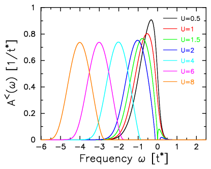
Figure 3: Local lesser Green’s function in equilibrium at $\beta=10$ and for different values of $U$.

The moments for the retarded and lesser Green’s functions are calculated by directly integrating the Green’s functions multiplied by the corresponding power of frequency; we use a step size of $\Delta\omega=0.001$ and a rectangular quadrature rule. The results for half-filling are presented in Table 1. One can immediately see that the numerical results for the first moment of the lesser Green’s function are in an excellent agreement with the exact expressions for the moment (the zeroth and second moments agreed exactly with their exact expressions). We also calculated the retarded moments and they agreed exactly with the exact values, so we don’t summarize them in a table. Note that there appears to be a relation between the second moments of the retarded and lesser Green’s functions at half filling. This relation ceases to hold off of half filling. For example, in the case with $U=2$, $w_{1}=0.25$, and $\rho_{e}=0.75$ we find the following moments (exact results in parentheses): $\tilde{\mu}_{1}^{R}=-0.872072144$ $(-0.872071963)$; $\tilde{\mu}_{2}^{R}=2.01050948$ $(2.01050951)$; $\tilde{\mu}_{1}^{<}=-2.149496$ $(-2.149462)$; and $\tilde{\mu}_{2}^{<}=3.623019$ $(3.622970)$. These results are more indicative of the general case (where $\tilde{\mu}_{2}^{R}\neq\tilde{\mu}_{2}^{<}$). Note that one needs to use many Matsubara frequencies in the summations to get good convergence for the average kinetic energy and for the second correlation function (we used 50,000 in this calculation with $\beta=10$). The majority of our numerical error comes from the difficulty in exactly calculating those results; indeed, the exact result, calculated from the operator averages on the Matsubara frequency axis is probably less accurate than the direct integration of the moment on the real axis. One can improve this situation somewhat by working on the real axis to calculate the different operator averages, but we wanted to indicate the accuracy under the most challenging circumstances. We feel our final results are quite satisfactory, and indicate these sum rules do hold.

Table 1: First spectral moment for the lesser Green’s function in equilibrium with $\beta=10$ and different values of $U$. The zeroth moment is accurate to more than eight digits, and is not included. Similarly, we find the second moment is equal to $0.5+U^{2}/4$ to high accuracy, and is not included. Note that the first moment continuously evolves from the value $-1/\sqrt{\pi}$ for $U=0$ and $\beta=\infty$ to approximately $-U/2$ as $U$ increases. The approach to $-U/2$ is expected due to the formation of upper and lower Hubbard bands separated by $U$.

moment	$U=0.5$	$U=1.0$	$U=1.5$	$U=2.0$	$U=4.0$	$U=6.0$
${\tilde{\mu}}_{1}^{<}$	-0.591699	-0.717901	-0.902869	-1.119047	-2.062036	-3.041526
${\tilde{\mu}}_{1}^{<}(exact)$	-0.591687	-0.717886	-0.902848	-1.119017	-2.061945	-3.041333

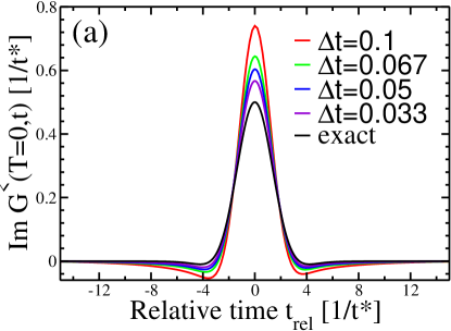
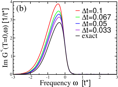
Figure 4: (Panel a) Imaginary part of the lesser Green’s function as a function of the relative time coordinate for different discretizations of the time contour. The model parameters are $U=0.5$, $\beta=10$ and $E=0$. The average time $T$ is set equal to zero. The parameters for the Kadanoff-Baym time-contour discretization are: $t_{max}=15$ and $\Delta\tau=0.1$ (i.e., 100 points taken along the imaginary axis); the discretization along the real time axis is given by $\Delta t$ as shown in the figure. Note how the results systematically approach the exact result as the discretization goes to zero. (Panel b) Imaginary part of the lesser Green’s function as a function of frequency for different discretizations of the time contour.

We now focus on numerical results for the nonequilibrium code. Our first benchmark is to calculate equilibrium results with that code and compare with exact results available for the equilibrium case. Such calculationsNashville show good convergence and precision when $U$ lies below the critical $U$ for the metal-insulator transition ($U<\sqrt{2}$). Here we demonstrate this by showing how the relative time dependence of the imaginary part of the lesser Green’s function at $U=0.5$ and $\beta=10$ changes when one decreases the time step $\Delta t$ on the real part of the Kadanoff-Baym contour. As follows from Fig. 4, the solution becomes more accurate as $\Delta t$ decreases but the accuracy is reduced as the temperature is lowered, as can be seen by comparing to the $\beta=1$ results in Ref. Nashville, . For this calculation, we determine the moments by taking the derivatives of the Green’s functions in the time representation. The values for the spectral moments at $U=0.5$, $\beta=10$ and different values of $\Delta t$ are presented in Tables 2 and 3. The results for the moments improve as $\Delta t$ decreases.

Table 2: Spectral moments for the retarded Green’s function in the case of zero electric field at $U=0.5$, $\beta=10$ and calculated with the nonequilibrium real-time formalism with different values for the time step $\Delta t$. The other parameters are $t_{max}=15$, $N=54,~{}55$, $\Delta\tau=0.1$

moment	$\Delta t=0.1$	$\Delta t=0.067$	$\Delta t=0.05$	$\Delta t=0.033$	exact
${\tilde{\mu}}_{0}^{R}$	1.580785	1.331640	1.232022	1.144811	1
${\tilde{\mu}}_{1}^{R}$	0.174040	0.082610	0.052785	0.030002	0
${\tilde{\mu}}_{2}^{R}$	1.324976	0.979230	0.848047	0.737020	0.5625

Table 3: The same as in Table III but for the case of the lesser Green’s function.

moment	$\Delta t=0.1$	$\Delta t=0.067$	$\Delta t=0.05$	$\Delta t=0.033$	exact
${\tilde{\mu}}_{0}^{<}$	1.480893	1.289036	1.207662	1.133850	1
${\tilde{\mu}}_{1}^{<}$	-1.036753	-0.850675	-0.774525	-0.706893	-0.591687
${\tilde{\mu}}_{2}^{<}$	1.108705	0.870853	0.777152	0.695791	0.5625

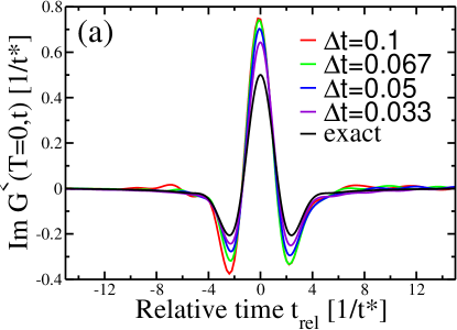
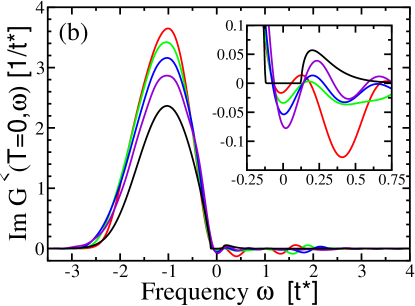
Figure 5: (Panel a) Imaginary part of the lesser Green’s function as a function of the relative time coordinate for different discretizations of the time contour. The model parameters are $U=2$, $\beta=10$ and $E=0$. The average time $T$ is set equal to zero. The parameters for the Kadanoff-Baym time-contour discretization are: $t_{max}=15$ and $\Delta\tau=0.1$ (i.e., 100 points taken along the imaginary axis); the discretization along the real time axis is given by $\Delta t$ as shown in the figure. Note how the results systematically approach the exact result as the discretization goes to zero. (Panel b) Imaginary part of the lesser Green’s function as a function of frequency for different discretizations of the time contour; in the inset, the region around $\omega=0$ is blown up to show the gap development as a function of the discretization. Note how the gap region converges very slowly—instead we see the DOS go negative in the gap region. Properly determining that structure in the frequency domain requires the Green’s function over an extended time domain, which is not numerically feasible.

In the insulating phase, the calculations are less accurate (see Fig. 5). The self-energy develops a pole in the frequency representation, which gives the imaginary part a delta function at the chemical potential. Hence, we expect a constant background value for the self-energy in the time representation. This cannot be properly represented in a numerical calculation that has a finite cutoff in the time domain, which makes the real-time formalism much more challenging in the insulating phase. The problems appear to be somewhat less pronounced for the Green’s functions, but the convergence is slower than in the metallic phase, and the gap region has unphysical behavior [the DOS goes negative in the gap region as shown in the inset to panel (b)]. One cannot get rid of these oscillations without having a time-domain cutoff that extends to infinity, but by comparing with the exact results, we find that a time-domain cutoff of about $t_{rel}\approx 200$ provides quite reasonable results for the calculations; in our results with the nonequilibrium code, we are limited to time-domain cutoffs of closer to $15-30$, which explains the poor agreement for the gap region. Fortunately, these numerical problems appear to reduce when an external field is turned on, and we are in the nonequilibrium case.

Note that we show equilibrium results only for the average time $T=0$. In equilibrium, the results should be independent of $T$, but we find that we have a modest $T$ dependence due to discretization error. The results at $T=0$ turn out to be the least accurate, and the accuracy of the results improves as the discretization size is made smaller. In general, we find the $T$ dependence of the Green’s functions to vary (pointwise) by no more than 40% for $\Delta t=0.1$ and to be reduced to a 10% variation when $\Delta t=0.033$ (for $U=0.5$). The variation is about three times larger for $U=2$. We find less variation in the nonequilibrium calculations, which appear to be better suited to the real-time formalism [most likely because the Green’s functions don’t behave like complex exponentials $\exp(i\epsilon t)$ as the equilibrium functions do; such functions can be particularly difficult to deal with in our real-time numerical calculations].

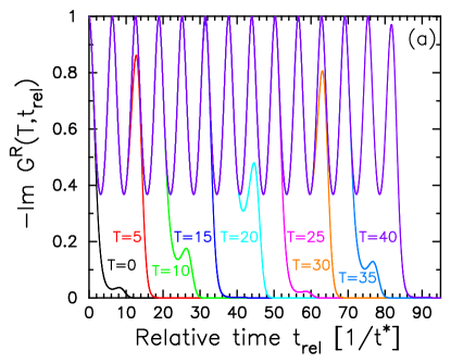
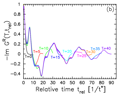
Figure 6: Imaginary part of the retarded Green’s function as a function of the relative time coordinate at different values of the average time (starting at $T=0$ and running to $T=40$ in steps of 5). The field is switched on at the time $T=0$ and we take $\Delta t=0.1$ along the Kadanoff-Baym contour. The model parameters are $\beta=10$ and $E=1$. Panel (a) shows the noninteracting result $U=0$, while panel (b) shows the interacting result $U=0.5$ (note that the curves extend as far out in $t_{rel}$ as we have data; the cutoff in $t_{rel}$ comes from the finite time domains of our calculations). Note how the results appear to retrace themselves for different average times until the relative time becomes larger than approximately $2T$, where the Green’s function decays. For the noninteracting case, the pattern obviously becomes periodic in the Bloch period as $T\rightarrow\infty$, which leads to delta functions in the Fourier transform (with respect to $t_{rel}$), whereas the interacting case may or may not be approaching a periodic form for large relative time; the data does not extend far enough out to be able to make a conclusion about the asymptotic form.

As a nonequilibrium problem, we consider the case of the interacting Falicov-Kimball model in the metallic phase at $U=0$ and $U=0.5$ with $\beta=10$ and a constant electric field $E=1$ is turned on at some moment of time. The Green’s functions for noninteracting electronsTurkowski [see panel (a) of Fig. 6] are oscillatory functions of the relative time coordinate in presence of the external field. The average time dependence is weak for relative times up to about $2T$, after which, the Green’s function decays as a function of $t_{rel}$. Notably, the results for different average times lie on top of each other until the relative time becomes larger than $2T$. This implies that there is little or no average time dependence to the retarded Green’s function as $T\rightarrow\infty$, and the retarded Green’s function becomes a periodic function of $t_{rel}$ (with the Bloch period); this latter result implies that the Fourier transform will consist of evenly spaced delta functions, which is the familiar Wannier-Stark ladder. When interactions are turned on, the situation changes [see panel (b) of Fig. 6]. We still see little average time dependence for relative times smaller than $2T$, but the Green’s function does not appear periodic in $t_{rel}$ for small times. The critical question to ask is, what happens as $T\rightarrow\infty$? If the Green’s function becomes periodic in $t_{rel}$, then there will be delta functions surviving in the Fourier transform, but if it continues to decay, there will not. Our data does not extend far enough out in time for us to be able to resolve this issue.

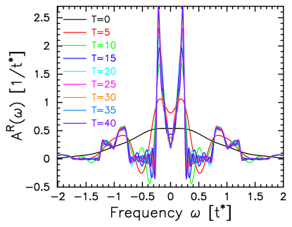
Figure 7: Density of states for different average times (running from $T=0$ to $T=40$ in steps of 5) for the interacting system, with $U=0.5$ and $E=1$. These results correspond to the Fourier transform of the data in Fig. 6. Note how the DOS seems to be approaching a limiting form even for this small a value of the average time. We cannot tell, however, whether there might be some low-weight delta functions appearing somewhere in the spectrum. In any case, it does appear that there are no sharp structures near the Bloch frequencies, which are at integer frequencies for $E=1$.

It is also interesting to examine the density of states in frequency space. The $U=0$ case has been studied exhaustively Turkowski , so we don’t repeat it here. The interacting case is plotted in Fig. 7. In constructing this plot, we set the real part of the retarded Green’s function to zero before performing the Fourier transform, since the exact result must vanish by particle-hole symmetry, and our numerical calculations have a small nonzero real part. Note how the DOS rapidly readjusts itself into a nonequilibrium form, and how the steady state appears to be approximately reached. The only subtle issue is the one discussed above, of whether there will be delta function peaks emerging in the DOS as the average time gets larger. What is clear, is that if such peaks do form, they are quite unlikely to appear at multiples of the Bloch frequencies, because we see no sharp peaks forming near integer frequencies here (the Bloch frequency is equal to 1 for $E=1$); indeed, the DOS seems to be suppressed at integer frequencies.

The lesser Green’s functions are remarkably similar to the retarded Green’s functions, except they are nonzero for all $t_{rel}$, not just for positive values. There also is limited average time dependence, except in the region of small $t_{rel}$, where the first derivative of the Green’s function does vary with average time. It is this variation that leads to oscillations in the current, and is critical for understanding the behavior of these systems. Unfortunately, it is not simple to directly evaluate such derivatives accurately when we calculate them numerically, because our time step is rather large. We examine them in this numerical fashion, with results plotted in Fig. 8 for the case $\Delta t=0.1$. Note how the first moment oscillates, then decays, and finally seems to reach a steady oscillatory state as the average time increases. We cannot tell whether the moment becomes a constant at large average times or continues to oscillate from the data that we have, although it appears to be approaching an oscillatory steady state. Note further that because $U$ is not too large here, we anticipate a correlation between these oscillations in the first moment and oscillations of the current. Indeed, if one calculates the current, one finds that it also appears to approach a steady oscillating state for large average time; details of these results will be presented elsewhere.

Figure 8: First moment of the local lesser function $\tilde{\mu}^{<}_{1}$ plotted as a function of average time T for $U=0.5$ and $E=1$. The field is turned on at $T=0$. The step size is $\Delta t=0.1$, and the moment is calculated from the numerical derivative of the data.

Despite a significant change in the Green’s functions after switching on an electric field (compare the $T=0$ results, which are close to the equilibrium results to the larger $T$ values in Figs. 6 and 7), the spectral moments for these functions do not change much (Tables 4 and 5). The spectral moments are connected with the relative time derivatives of the Green’s functions [Eq. (18)]; the fact that some moments do not change in the presence of an electric field suggests that the those derivatives are independent of the electric field. Indeed, we calculate the moments in these examples from the derivatives of the Green’s functions at $t=0$ because we often do not have data out to a large enough relative time to perform the Fourier transform, and evaluate the moment in the conventional way. Note that, the second moment, which is actually equal to the curvature of $G^{R}$ and $G^{<}$, is independent of average time for the retarded function, and does not appear to have average time dependence for the lesser function. The first moment of the lesser function does depend on average time (see Fig. 8). Finally, it is interesting to observe that the values for the moments are much closer to the exact results for a similar discretization size than what we found in the equilibrium case. This is why we believe that the real-time numerical algorithm converges better for the nonequilibrium case than for the equilibrium case.

Table 4: Spectral moments for the retarded Green’s function in the case when the constant external electric field $E=1$ is switched on at $T=0$. The parameters are $U=0.5$, $\beta=10$, $\Delta t=0.05$, $t_{max}=15$, $N=54,~{}55$, and $\Delta\tau=0.05$. These moments should all be independent of time, and they appear to be within the numerical error.

moment	T=0	T=5	T=10	T=15	T=20	exact
${\tilde{\mu}}_{0}^{R}$	1.0025	1.0088	0.9985	0.9951	0.9967	1
${\tilde{\mu}}_{1}^{R}$	0.00665	-0.00054	0.00005	0.00054	0.00003	0
${\tilde{\mu}}_{2}^{R}$	0.56155	0.56198	0.55184	0.55030	0.55112	0.5625

Table 5: The same as in Table IV for the case of the lesser Green’s function. The first moment appears to change with average time in the nonequilibrium case. The equilibrium value is $-0.5917$, which agrees well with our result before the field is turned on. The second moment appears to be independent of average time, even in a field, but we have no proof of this fact.

moment	T=0	T=5	T=10	T=15	T=20	exact
${\tilde{\mu}}_{0}^{<}$	1.0025	1.0098	0.9997	0.9960	0.9975	1
${\tilde{\mu}}_{1}^{<}$	-0.5878	0.0042	-0.1618	-0.0454	0.0933	?
${\tilde{\mu}}_{2}^{<}$	0.5520	0.5666	0.5554	0.5572	0.5588	?

To conclude our numerical analysis, we consider the spectral moments of the lesser Green’s function in the case where it is approximated by the generalized Kadanoff-Baym (GKB) ansatzLipavsky . The idea of the GKB is to represent the lesser Green’s function in terms of the distribution function (determined by the $t=0$ limit of the lesser Green’s function) and the full two-time retarded and advanced Green’s functions:

$$\hat{G}_{{\bf k}}^{<}(t_{1},t_{2}) = -i\left[G_{{\bf k}}^{R}(t_{1},t_{2})G_{{\bf k}}^{<}(t_{2},t_{2})\right.$$ (65)

$$- \left.G_{{\bf k}}^{<}(t_{1},t_{1})G_{{\bf k}}^{A}(t_{1},t_{2})\right].$$

The expression for the spectral moments of the lesser Green’s function, approximated by Eq. (65), can be found by taking relative time derivatives of $\hat{G}_{{\bf k}}^{<}(T,t)$ as shown in Eq. (18). Similar to the derivation performed in Section II, one finds (the hat denotes the GKB approximation)

$$\hat{\mu}_{0}^{<}({\bf k},T) = 2n_{c}({\bf k},T),$$ (66)

$$\hat{\mu}_{1}^{<}({\bf k},T) = n_{c}({\bf k},T)\left(\left\langle\left\{[c_{{\bf k}}(T),H],c_{{\bf k}}^{\dagger}(T)\right\}\right\rangle\right.$$ (67)

$$- \left.\left\langle\left\{c_{{\bf k}}(T),[c_{{\bf k}}^{\dagger}(T),H]\right\}\right\rangle\right)$$

$$+ {\rm Im}\frac{\partial n_{c}({\bf k},T)}{\partial T},$$

$$\hat{\mu}_{2}^{<}({\bf k},T) = \frac{1}{2}n_{c}({\bf k},T)\left(\left\langle\left\{[[c_{{\bf k}}(T),H],H],c_{{\bf k}}^{\dagger}(T)\right\}\right\rangle\right.$$ (68)

$$- 2\left.\left\langle\left\{[c_{{\bf k}}(T),H],[c_{{\bf k}}^{\dagger}(T),H]\right\}\right\rangle\right.$$

$$+ \left.\left\langle\left\{c_{{\bf k}}(T),[[c_{{\bf k}}^{\dagger}(T),H],H]\right\}\right\rangle\right)$$

$$- \frac{1}{2}{\rm Re}\frac{\partial^{2}n_{c}({\bf k},T)}{\partial T^{2}}.$$

Comparison of the expressions in Eqs. (66)–(68) for the GKB moments with the corresponding exact expressions in Eqs. (19), (22) and (25) for the moments of $G_{{\bf k}}^{R}$ allows us to connect the lesser GKB spectral moments with the exact retarded spectral moments:

$$\hat{\mu}_{n}^{<}({\bf k},T)=2n_{c}({\bf k},T)\mu_{n}^{R}({\bf k},T)-\delta_{n,2}\frac{1}{2}\frac{\partial^{2}n_{c}({\bf k},T)}{\partial T^{2}},$$ (69)

for $n=0$, 1, and 2. Since the time derivatives of the momentum distribution function are real valued, the last term in Eq. (69) is nonzero only for $n=2$. Thus, the lesser GKB spectral moments (with $n=0$, 1, and 2) are equal to the corresponding retarded spectral moments multiplied by $2n_{c}({\bf k},T)$ plus a term involving the second time derivative of the momentum distribution function for the case of $n=2$.

Comparison of Eq. (69) and the exact expressions for the retarded spectral moments [in Eqs. (19), (23) and (II)] with the exact expressions for the lesser moments [in Eqs. (33), (37) and (II)] allows us to conclude that the lesser spectral moments for the GKB approximated Green’s function correspond to an approximation of the exact spectral moments by evaluating the operator averages with a mean-field approximation (the second moment contains an additional term with the second time derivative of the momentum distribution function). This indicates that the GKB approximation will fail as the correlations increase, because it produces the wrong moments to the spectral functions. Note that this does not say the GKB approach is a mean field theory approach, it is not.

IV Conclusions

In this paper, we derived a sequence of spectral moment sum rules for the retarded and lesser Green’s functions of the Falicov-Kimball and Hubbard models. Our analysis holds in equilibrium and in the nonequilibrium case of a spatially uniform, but time-dependent external electric field being applied to the system. Our results are interesting, because they show there is no average time dependence nor electric field dependence to the first three moments of the local retarded Green’s functions. This implies that the value, slope and curvature of the local retarded Green’s functions, as functions of the relative time, do not depend on the average time or the field. Such a result extends the well-known result that the total spectral weight (zeroth moment) of the Green’s function is independent of the field. It also implies that one will only see deviations of Green’s functions from the equilibrium results when the relative time becomes large. Such an observation is quite useful for quantifying the accuracy of nonequilibrium calculations. We showed some numerical results illustrating this effect for nonequilibrium DMFT calculations in the Falicov-Kimball model. The case for the lesser Green’s function is more complicated, and there is both average time dependence and field dependence apparent in those moments, although it appears that the second moment at half filling may not depend on average time.

We also examined a common approximation employed in nonequilibrium calculations, the so-called generalized Kadanoff-Baym ansatz. We find the moments in that case are similar in form to the exact moments, except they involve a mean-field-theory decoupling of correlation function expectation values when one evaluates the operator averages that yield the sum-rule values. This implies that the GKB approximation must fail as the correlations increase, and such a mean-field decoupling becomes inaccurate, because it will have the wrong spectral moments.

We hope that use of these spectral moments will become common in nonequilibrium calculations in order to quantify the errors of the calculations for small times. We believe they can be quite valuable in checking the fidelity of numerical calculations and of different kinds of approximate solutions.

Appendix A Derivation of the second spectral moment for the retarded Green’s function

We show the explicit steps needed to derive Eq. (25) by using Eqs. (14) and (7) for the second spectral moment of the retarded Green’s function. In this case, the second spectral moment is equal to

$$\mu_{2}^{R}({\bf k},T)=\left(-\frac{1}{\pi}\right)\int_{-\infty}^{\infty}d\omega{\rm Im}\int_{-\infty}^{\infty}dte^{i\omega t}i\frac{\partial^{2}}{\partial t^{2}}\left[\theta(t)\left\langle\left\{c_{{\bf k}}\left(T+\frac{t}{2}\right),c_{{\bf k}}^{\dagger}\left(T-\frac{t}{2}\right)\right\}\right\rangle\right].$$ (70)

This expression is equivalent to

$$\mu_{2}^{R}({\bf k},T) = -\frac{1}{\pi}\int_{-\infty}^{\infty}d\omega{\rm Im}\int_{-\infty}^{\infty}dte^{i\omega t}i\frac{\partial\delta(t)}{\partial t}\left\langle\left\{c_{{\bf k}}\left(T+\frac{t}{2}\right),c_{{\bf k}}^{\dagger}\left(T-\frac{t}{2}\right)\right\}\right\rangle$$ (71)

$$- \frac{1}{\pi}\int_{-\infty}^{\infty}d\omega{\rm Im}\int_{-\infty}^{\infty}dte^{i\omega t}\delta(t)\left[\left\langle\left\{i\frac{\partial}{\partial t}c_{{\bf k}}\left(T+\frac{t}{2}\right),c_{{\bf k}}^{\dagger}\left(T-\frac{t}{2}\right)\right\}\right\rangle\right.+\left.\left\langle\left\{c_{{\bf k}}\left(T+\frac{t}{2}\right),i\frac{\partial}{\partial t}c_{{\bf k}}^{\dagger}\left(T-\frac{t}{2}\right)\right\}\right\rangle\right]$$

$$+ \frac{1}{\pi}\int_{-\infty}^{\infty}d\omega{\rm Im}\int_{-\infty}^{\infty}dte^{i\omega t}i\theta(t)\left[\left\langle\left\{i^{2}\frac{\partial^{2}}{\partial t^{2}}c_{{\bf k}}\left(T+\frac{t}{2}\right),c_{{\bf k}}^{\dagger}\left(T-\frac{t}{2}\right)\right\}\right\rangle\right.$$

$$+ \left.2\left\langle\left\{i\frac{\partial}{\partial t}c_{{\bf k}}\left(T+\frac{t}{2}\right),i\frac{\partial}{\partial t}c_{{\bf k}}^{\dagger}\left(T-\frac{t}{2}\right)\right\}\right\rangle+\left\langle\left\{c_{{\bf k}}\left(T+\frac{t}{2}\right),i^{2}\frac{\partial^{2}}{\partial t^{2}}c_{{\bf k}}^{\dagger}\left(T-\frac{t}{2}\right)\right\}\right\rangle\right].$$

The first two integrals in Eq. (71) are equal to zero, that is,

$$- \frac{1}{\pi}\int_{-\infty}^{\infty}d\omega{\rm Im}\int_{-\infty}^{\infty}dte^{i\omega t}i\frac{\partial\delta(t)}{\partial t}$$ (72)

$$\times \left\langle\left\{c_{{\bf k}}\left(T+\frac{t}{2}\right),c_{{\bf k}}^{\dagger}\left(T-\frac{t}{2}\right)\right\}\right\rangle=0,$$

and

$$- \frac{1}{\pi}\int_{-\infty}^{\infty}d\omega{\rm Im}\int_{-\infty}^{\infty}dte^{i\omega t}\delta(t)$$ (73)

$$\times \left[\left\langle\left\{i\frac{\partial}{\partial t}c_{{\bf k}}\left(T+\frac{t}{2}\right),c_{{\bf k}}^{\dagger}\left(T-\frac{t}{2}\right)\right\}\right\rangle\right.$$

$$+ \left.\left\langle\left\{c_{{\bf k}}\left(T+\frac{t}{2}\right),i\frac{\partial}{\partial t}c_{{\bf k}}^{\dagger}\left(T-\frac{t}{2}\right)\right\}\right\rangle\right]=0.$$

To prove Eq. (72), we note that the delta-function derivative satisfies

$$\int_{-\infty}^{\infty}dtf(t)\frac{\partial\delta(t-a)}{\partial t}=-f^{\prime}(a).$$ (74)

Hence, we can transfer the time derivative of the delta function into a time derivative of the other factors in the integrand. This time derivative has two terms: (i) the first term is the derivative of the exponential, which introduces an additional factor of $i\omega$ (the operator average then becomes trivial when we set $t=0$, since the anticommutator is equal to 1) and (ii) the second term which involves derivatives of the creation and annihilation operators. Performing the integration over $t$ by using the delta function then yields

$$- \frac{1}{\pi}\int_{-\infty}^{\infty}d\omega\Biggr{(}{\rm Im}(\omega)-{\rm Im}\left[\left\langle\left\{[c_{{\bf k}}(T),\mathcal{H(T)}],c_{{\bf k}}^{\dagger}(T)\right\}\right\rangle\right.$$ (75)

$$-\left.\left\langle\left\{c_{{\bf k}}(T),[c_{{\bf k}}^{\dagger}(T),\mathcal{H(T)}]\right\}\right\rangle\right]\Biggr{)},$$

where we replaced derivatives with respect to time by commutators with the Hamiltonian. The first term has no imaginary part, so it vanishes, as do the second two terms, since one can easily show the difference of the two operators is Hermitian, and hence has a real expectation value. This completes the proof of Eq. (72).

To prove (73), we first perform the integration over $t$. The result is equal to

$$- \frac{1}{\pi}\int_{-\infty}^{\infty}d\omega{\rm Im}\frac{1}{2}\left[\left\langle\left\{i\frac{\partial}{\partial T}c_{{\bf k}}(T),c_{{\bf k}}^{\dagger}(T)\right\}\right\rangle\right.$$ (76)

$$- \left.\left\langle\left\{c_{{\bf k}}(T),i\frac{\partial}{\partial T}c_{{\bf k}}^{\dagger}(T)\right\}\right\rangle\right]$$

$$= -\frac{1}{\pi}\int_{-\infty}^{\infty}d\omega{\rm Im}\frac{1}{2}\left\langle\left[\left\{[c_{{\bf k}}(T),\mathcal{H}(T)],c_{{\bf k}}^{\dagger}(T)\right\}\right.\right.$$

$$- \left.\left.\left\{c_{{\bf k}}(T),[c_{{\bf k}}^{\dagger}(T),\mathcal{H}(T)]\right\}\right]\right\rangle.$$

The operator in the second line of Eq. (76) is the same operator we saw above; it is Hermitian so the imaginary part of the statistical average vanishes. This proves (73).

To complete the derivation of the second spectral moment, we note that only the last integral term in Eq. (71) can be nonzero. Substituting the operator time derivatives by their commutators with the Hamiltonian finally gives the expression in Eq. (25) of the second spectral moment for the retarded Green’s function.

References

- (1) J. Hubbard, Proc. Royal Soc. A 276, 238 (1963).
- (2) L. M. Falicov and J. C. Kimball, Phys. Rev. Lett. 22, 997 (1969).
- (3) E. H. Lieb and F. Y. Wu, Phys. Rev. Lett. 20, 1445 (1968).
- (4) A. Georges, G. Kotliar, W. Krauth, and M. J. Rozenberg, Rev. Mod. Phys. 68, 13 (1996).
- (5) J. K. Freericks and V. Zlatić, Rev. Mod. Phys. 75, 1333 (2003).
- (6) S. R. White, Phys. Rev. B 44, 4670 (1991).
- (7) P. Schmidt and H. Monien, preprint cond-mat/0202046; P. Schmidt, diplome thesis, University of Bonn (2002).
- (8) U. Brandt and M. P. Urbanek, Z. Phys. B–Condens. Mat. 89, 297 (1992).
- (9) J. K. Freericks, V. M. Turkowski and V. Zlatić, “Real-time formalism for studying the non-linear response of ”smart” materials to an electric field.” To be published in Proceedings of the 2005 Users Group Conference, IEEE Computer Society, Nashville, Tennessee (2005).
- (10) V. Turkowski and J. K. Freericks, Phys. Rev. B 71, 085104 (2005).
- (11) J. K. Freericks, V. M. Turkowski, and V. Zlatić, Phys. Rev. B 71, 115111 (2005).
- (12) R. E. Peierls, Z. Phys. 80, 763 (1933); A. P. Jauho and J. W. Wilkins, Phys. Rev. B 29, 1919 (1984).
- (13) R. Bertoncini and A. P. Jauho, Phys. Rev. B 44, 3655 (1991).
- (14) S. Elitzur, Phys. Rev. D 12, 3978 (1975); V. Subrahmanyam and M. Barma, J. Phys. C 21, L19 (1988).
- (15) J. K. Freericks and V. Zlatić, Phys. Rev. B 64, 245118 (2001); (E) Phys. Rev. B 66, 249901 (2002).
- (16) D. C. Langreth, in Linear and Nonlinear Electron Transport in Solids, edited by J. T. Devreese and V. E. van Doren (Plenum Press, New York and London, 1976).
- (17) U. Brandt and C. Mielsch, Z. Phys. B–Condens. Mat. 75, 365 (1989).
- (18) W. Metzner, Phys. Rev. B 43, 8549 (1991).
- (19) W. Metzner and D. Vollhardt, Phys. Rev. Lett. 62, 324 (1989).
- (20) J. K. Freericks, V. M. Turkowski, and V. Zlatić, unpublished.
- (21) P. Lipavský, V. Spicka, and B. Velický, Phys. Rev. B 34, 6933 (1986).