Schrödinger-Chern-Simons Vortex Dynamics

Abstract

We study the motion of vortices in the planar Ginzburg-Landau model with Schrödinger-Chern-Simons dynamics. We compare the moduli space approximation with the results of numerical simulations of the full field theory and find that there is agreement if the coupling constant is very close to the critical value separating Type I from Type II superconductors. However, there are significant qualitative differences even for modest deviations from the critically coupled regime. Radiation effects produce forces which are of the same order of magnitude as the intervortex force and therefore have a significant impact on vortex motion. We conclude that the moduli space approximation does not provide a good description of the dynamics in this regime.

1 Introduction

The planar Ginzburg-Landau model provides a good mathematical description of the static properties of vortices in thin superconductors, but in order to describe vortex motion this needs to be supplemented by some appropriate dynamics. There are several possibilities for the form of this dynamics and it is currently difficult to determine which of these is the closest to modelling real superconductors, since in experimental situations the vortices are often pinned, so it is difficult to identify the underlying dynamical behaviour.

It has been argued [1] that at very low temperatures dissipation can be ignored and vortex motion is orthogonal to the force acting, so that two vortices circulate around each other, as in a fluid. An interesting Lagrangian field theory to describe this type of behaviour has been proposed by Manton [4] in which the potential part is the usual Ginzburg-Landau energy and the kinetic terms are linear in the time derivatives of the complex scalar field and contain a Chern-Simons term. The equation of motion for the complex scalar field is a gauged Schrödinger equation, hence the name Schrödinger-Chern-Simons dynamics. It is Manton’s model that we shall study in this paper.

At critical coupling, which separates Type I from Type II superconductors, minimizers of the Ginzburg-Landau potential energy are static solutions of the Schrödinger-Chern-Simons equations, so there is no vortex motion. Thus to investigate vortex dynamics the model needs to be studied away from critical coupling.

The moduli space approximation [3] to soliton dynamics, in which the field theory dynamics is approximated by motion on a finite dimensional manifold, has been applied to Schrödinger-Chern-Simons vortex dynamics [4, 8]. The moduli space used is the manifold of static vortices at critical coupling, so it should be most accurate when the coupling constant is close to its critical value, though it can not equal this value if there is to be vortex motion, as mentioned above. In particular, it predicts that indeed two vortices circulate around each other at constant speed, and provides an expression for the period of this motion in terms of quantities defined on the moduli space. Polygonal configurations of $N$ vortices can also be studied and the moduli space approximation predicts that for well separated vortices these symmetric configurations are stable if and only if $N<6.$

In this paper we perform numerical simulations of the full field theory dynamics and compare the results with the predictions of the moduli space approximation. For two vortices we find that there is a good agreement when the coupling constant is very close to the critical value. However, there are significant qualitative differences even for modest deviations away from critical coupling. We find that two vortices move on spirals, rather than circles, and spiral in or out depending upon the value of the coupling constant. This behaviour is due to radiation effects which are neglected in the moduli space approximation but turn out to produce forces which are of the same order of magnitude as the intervortex force. Polygonal arrangements also exhibit the same spiral phenomenon and the stability properties do not always agree with the moduli space predictions.

2 The Schrödinger-Chern-Simons Model

The Ginzburg-Landau potential energy is given by

$$V=\frac{1}{2}\int\left(B^{2}+\overline{D_{i}\phi}D_{i}\phi+\frac{\lambda}{4}(1-\overline{\phi}\phi)^{2}\right)d^{2}x,$$ (2.1)

where $\phi$ is a complex scalar field, representing the electron pair condensate, and the covariant derivative is $D_{i}\phi=\partial_{i}\phi-ia_{i}\phi,$ formed using the abelian gauge potential $a_{i}$ with an associated magnetic field

$$B=\partial_{1}a_{2}-\partial_{2}a_{1}.$$ (2.2)

In (2.1), and the following, the summation convention applies to the two spatial indices only, ie. $i=1,2.$

The finite energy topological solitons of this model are known as vortices. The vortex number $N$ is a topological degree and is equal to the total magnetic flux in units of $2\pi$,

$$N=\frac{1}{2\pi}\int B~{}d^{2}x.$$ (2.3)

$N$ is also equal to the total number of zeros of the complex scalar field $\phi$ counted with multiplicity. These zeros can be interpreted as the vortex positions when the vortices are well separated.

The positive parameter $\lambda$ plays a crucial role in the properties of the model and its vortex solutions. For $\lambda<1$ the superconductor is of Type I and the potential energy $V$ of two vortices is an increasing function of their separation ie. vortices attract.

For $\lambda>1$ the superconductor is of Type II and the potential energy of two vortices is a decreasing function of their separation ie. vortices repel. At the critical coupling $\lambda=1,$ separating Type I from Type II superconductors, the potential energy is independent of their separation. Moreover, at critical coupling, and for all positive vortex numbers $N,$ the parameter space of all minimal energy $N$-vortices forms a $2N$-dimensional smooth manifold, known as the moduli space $M_{N}$. In this case the potential energy of any $N$-vortex solution is equal to $\pi N$ for arbitrary values of the vortex positions.

At critical coupling the second order field equations which follow from the variation of the potential (2.1) can be reduced to two first order Bogomolny equations

$$D_{1}\phi+iD_{2}\phi = 0,$$ (2.4)

$$B-\frac{1}{2}(1-\overline{\phi}\phi) = 0,$$ (2.5)

and these will play an important role later.

The Schrödinger-Chern-Simons model introduced by Manton [4] is a non-dissipative model for vortex motion in thin superconductors. The model is defined by the Lagrangian

$$L=\int\left(\frac{i}{2}\left(\overline{\phi}D_{0}\phi-\phi\overline{D_{0}\phi}\right)+(Ba_{0}+e_{1}a_{2}-e_{2}a_{1})-a_{0}\right)d^{2}x-V,$$

where we have scaled some possible parameters to convenient values and $e_{i}$ is the electric field $e_{i}=\partial_{0}a_{i}-\partial_{i}a_{0}.$ Note that the term $Ba_{0}+e_{1}a_{2}-e_{2}a_{1}$ is simply the Chern-Simons term written out explicitly and that the $-a_{0}$ term is required to allow the possibility of a condensate at infinity. The potential term $V$ of the Lagrangian (2) is the Ginzburg-Landau energy (2.1). This Lagrangian is both gauge invariant and Galilean invariant, when one takes into account a constant external transport current. Although this is an important feature of the model we shall not be concerned with this aspect here.

The equations of motions which follow from (2) are given by

$$iD_{0}\phi = -\frac{1}{2}D_{i}D_{i}\phi-\frac{\lambda}{4}(1-\overline{\phi}\phi)\phi,$$ (2.6)

$$-\varepsilon_{ij}\partial_{j}B = \frac{i}{2}\left(\overline{\phi}D_{i}\phi-\phi\overline{D_{i}\phi}\right)+2\varepsilon_{ij}e_{j},$$ (2.7)

$$B = \frac{1}{2}(1-\overline{\phi}\phi).$$ (2.8)

The first equation is a gauge covariant nonlinear Schrödinger equation. The second equation is an Ampère equation, where the total current is the sum of the usual supercurrent and a Hall current orthogonal to the electric field. The third equation is a generalized Gauss law, which contains no time derivatives. It can be interpreted as a constraint on the initial data since it can be shown that the first two equations already imply that it is conserved, namely,

$$\frac{\partial}{\partial t}\left(B-\frac{1}{2}(1-\overline{\phi}\phi)\right)=0.$$ (2.9)

Therefore, once equation (2.8) is satisfied for the initial data, equations (2.6) and (2.7) guarantee that it is satisfied for all later times.

As the Lagrangian is linear in time derivatives then the kinetic energy makes no contribution to the conserved energy, which is simply the potential energy $V,$ whose conservation is easily checked using the equations of motion.

If the Schrödinger equation (2.6) and the Ampère equation (2.7) are considered for static fields, with a vanishing time component for the gauge potential $a_{0}=0,$ then these two equations reduce to the two second order field equations obtained from the variation of the Ginzburg-Landau energy (2.1). However, away from critical coupling, these static Ginzburg-Landau vortices will not satisfy the Gauss law (2.8) and hence are not static solutions of the Schrödinger-Chern-Simons equations. The exception is at critical coupling $\lambda=1$ where Ginzburg-Landau vortices also satisfy the Bogomolny equations (2.4) and (2.5), the second of which is precisely the Gauss law (2.8).

The first issue to consider is therefore the static solutions of the Schrödinger-Chern-Simons model away from critical coupling. We shall restrict to axially symmetric solutions, since it is expected that all static solutions will have axial symmetry when $\lambda\neq 1.$ We work in the radial gauge $a_{r}=0,$ with $a_{\theta}(r)$ and $a_{0}(r)$ functions of the radius $r$ only, and the complex scalar field having the standard $N$-vortex form $\phi=f(r){\rm e}^{iN\theta},$ where $f(r)$ is the radial profile function.

Substituting this axial ansatz into the field equations (2.6), (2.7) and (2.8) yields the following set of ordinary differential equations

$$f^{\prime\prime}+\frac{1}{r}f^{\prime}-\frac{1}{r^{2}}\left(N-a_{\theta}\right)^{2}f+\frac{\lambda}{2}\left(1-f^{2}\right)f+2a_{0}f=0,$$ (2.10)

$$\left(\frac{1}{r}a_{\theta}^{\prime}\right)^{\prime}+\frac{1}{r}\left(N-a_{\theta}\right)f^{2}-2a_{0}^{\prime}=0,$$ (2.11)

$$\frac{2}{r}a_{\theta}^{\prime}+f^{2}-1=0,$$ (2.12)

where $\prime$ denotes differentiation with respect to $r$. The boundary conditions for the fields are $f(0)=0$, $f(\infty)=1$, $a_{\theta}(0)=0$, $a_{\theta}(\infty)=N$ and $a_{0}^{\prime}(0)=0.$ Note that from (2.10) these boundary conditions automatically imply that $a_{0}(\infty)=0.$

Figure 1: Graphs of the functions $f(r)$, $a_{\theta}(r)$ and $a_{0}(r)$ for couplings $\lambda=1$ (solid curves), $\lambda=0.5$ (dashed curves), $\lambda=2$ (dotted curves).

These equations are solved using a gradient flow method with a fictitious energy constructed from the square of the field equations. The results for the $N=1$ vortex are displayed in Fig. 1, for three values of the coupling constant; $\lambda=1$ (solid curves), $\lambda=0.5$ (dashed curves), $\lambda=2$ (dotted curves). The critical coupling case $\lambda=1$ is shown for comparison, where $a_{0}=0$ and the functions $f(r)$ and $a_{\theta}(r)$ are the usual fields of the Ginzburg-Landau vortex. The qualitative features of both the profile function $f(r)$ and the angular component of the gauge field $a_{\theta}(r)$ do not vary significantly away from critical coupling. If $\lambda<1$ then $f(r)$ is slightly wider and $a_{\theta}(r)$ is a little narrower, with the opposite being true for $\lambda>1,$ that is, $f(r)$ is narrower and $a_{\theta}(r)$ is wider. The most significant feature is the behaviour of the temporal component of the gauge potential $a_{0},$ which is positive for $\lambda<1$ and negative for $\lambda>1.$ Thus, away from critical coupling, vortices not only have a magnetic field but also a tiny electric field. For a single vortex the electic field is radial and positive if $\lambda<1,$ whereas it is negative if $\lambda>1.$

Figure 2: The energy per vortex (in units of $\pi$) as a function of the coupling $\lambda$ for the axial $N$-vortex with $N=1$ (solid curve), $N=2$ (dased curve), $N=3$ (dotted curve).

As we have mentioned earlier, the conserved energy in the Schrödinger-Chern-Simons model is the Ginzburg-Landau energy $V.$ However, for $\lambda\neq 1$ the static fields are not those of the Ginzburg-Landau model, so the energy dependence on $\lambda,$ for varying vortex numbers $N,$ can not be inferred from knowledge of the Ginzburg-Landau model. In Fig. 2 we plot the energy per vortex (in units of $\pi$) of the axial $N$-vortex as a function of $\lambda$ for $N=1$ (solid curve), $N=2$ (dashed curve), $N=3$ (dotted curve). We have also computed similar results for larger values of $N,$ but for clarity they are not shown on this plot.

Despite the above comment we find that the qualitative behaviour of the energy is similar to Ginzburg-Landau vortices. In particular, for multi-vortices we see that for $\lambda<1$ the energy of $N$ well separated vortices is higher than the energy of an axially symmetric charge $N$ vortex, so vortices are attractive in this sense. For $\lambda>1$ vortices are repulsive, in that the energy of $N$ well separated vortices is lower than the charge $N$ axial configuration. At critical coupling, $\lambda=1,$ the static vortices coincide with Ginzburg-Landau vortices, so the energy per vortex equals $\pi$ for all $N,$ as it does for all vortices in the $2N$-dimensional moduli space $M_{N}$.

The above features of the vortex interaction energy will play an important role in the dynamics of vortices, as we shall see later.

3 The Moduli Space Approximation

The main idea of the moduli space approximation [3] is to project the dynamics of the full field theory onto a suitable finite dimensional space of field configurations. In the simplest situation, such as vortices at critical coupling or BPS monopoles, this finite dimensional space is the moduli space of static minimal energy solutions, with a given soliton number. This approach is well established (for a review see [6]) for relativistic Lagrangians, where the dynamics is second order in time. Restricting the field theory Lagrangian to the moduli space produces (upto an irrelevant constant) a purely kinetic Lagrangian on the moduli space, which may be interpreted as the moduli space metric. The slow motion of solitons is approximated by geodesic motion with respect to this metric. For relativistic dynamics of Ginzburg-Landau vortices in the abelian Higgs model the validity of this approximation has been proved with mathematical rigour [13].

A slightly more complicated situation arises if a theory is considered at parameter values for which the moduli space of static solutions is not large enough to describe solitons with arbitrary positions, for example, vortices in the abelian Higgs model away from critical coupling. In such situations the dynamics can be truncated to motion on the moduli space of the theory at critical coupling, but now there will also be a potential energy function on the moduli space, so the dynamics is no longer described by geodesic motion. This approach has been applied in different models [14, 10], and there is a good agreement with results obtained from numerical simulations of the full relativistic field theory dynamics. For relativistic vortex dynamics near to critical coupling rigourous error estimates can again be obtained [13].

Schrödinger-Chern-Simons vortex dynamics is first order in time, so initial conditions consist only of vortex positions. Furthermore, at critical coupling the Ginzburg-Landau vortices are static solutions, so there is no vortex motion. Thus, in constrast to relativistic dynamics, it is necessary to move away from critical coupling in order for there to be any vortex dynamics to study. Manton has argued [4] that it is possible to use moduli space techniques to describe Schrödinger-Chern-Simons vortex dynamics close to critical coupling, and this has been further investigated in some detail by Romão and Speight[8]. We summarise the results of the relevant calculations below.

Let $q^{\alpha}$, for $\alpha=1,\ldots,2N,$ be real coordinates on the moduli space $M_{N},$ for example the real and imaginary parts of the vortex positions when space is identified with the complex plane. As the Schrödinger-Chern-Simons Lagrangian (2) depends only linearly on time derivatives then the Lagrangian restricted to the moduli space must have the form

$$L_{\mbox{red}}={\cal A}_{\alpha}(q)\dot{q}^{\alpha}-V_{\mbox{red}}(q),$$ (3.1)

where ${\cal A}_{\alpha}(q)$ may be interpreted as the components of a $U(1)$ connection form ${\cal A}={\cal A}_{\alpha}dq^{\alpha}$ on $M_{N}.$ The first order equations of motion which follow from (3.1) are

$${\cal F}_{\alpha\beta}\dot{q}^{\alpha}=-\frac{\ \partial V_{\mbox{red}}}{\partial q^{\beta}},$$ (3.2)

where ${\cal F}=d{\cal A}$ is the curvature form of ${\cal A}.$ In order to study the details of this reduced dynamics we first need a better understanding of the moduli space $M_{N}$.

By considering the Bogomolny equations (2.4) and (2.5) Taubes [15] showed that it is possible to eliminate the gauge potential as follows. Define

$$h=\log|\phi|^{2},$$ (3.3)

which is gauge invariant and finite, except at the zeros of $\phi$. Using the first Bogomolny equation (2.4), it can be shown that the magnetic field can be expressed as

$$B=-\frac{1}{2}\nabla^{2}h.$$ (3.4)

The second Bogomolny equation then becomes

$$\nabla^{2}h+1-{\rm e}^{h}=0.$$ (3.5)

Recall $h$ has logarithmic singularities at the zeros of $\phi$. This can be accounted for by including delta-function sources into the equation,

$$\nabla^{2}h+1-{\rm e}^{h}=4\pi\sum\limits_{r=1}^{N}\delta(z-Z_{r}),$$ (3.6)

where $\delta$ is the two dimensional delta-function and $Z_{r},$ with $r=1,\ldots,N.,$ are the complex positions of the zeros of $\phi$ in $\hbox{\mybb R}^{2},$ which is identified with the complex plane. It can be shown that $h$ has the following expansion around a zero $z=Z_{r}$

$$h(z,\overline{z})=2\log|z-Z_{r}|+a_{r}+\frac{1}{2}\overline{b}_{r}(z-Z_{r})+\frac{1}{2}b_{r}(\overline{z}-\overline{Z}_{r})+O(|z-Z_{r}|^{2}).$$ (3.7)

It turns out that the coefficients $b_{r}$ contain all the necessary information to reconstruct the geometry of the moduli space.

Following the work of Strachan [12], Samols [9] was able to show that the moduli space metric derived from vortex dynamics in the relativistic abelian Higgs model is given by

$$ds^{2}=\pi\sum\limits_{r,s=1}^{N}\left(\delta_{rs}+2\frac{\partial b_{s}}{\partial Z_{r}}\right)dZ_{r}d\overline{Z}_{s},$$ (3.8)

which is a Kähler metric. The corresponding Kähler form is

$$\omega=\frac{i\pi}{2}\sum\limits_{r,s=1}^{N}\left(\delta_{rs}+2\frac{\partial b_{s}}{\partial Z_{r}}\right)dZ_{r}\wedge d\overline{Z}_{s}.$$ (3.9)

and it turns out that the curvature form ${\cal F},$ which appears in Schrödinger-Chern-Simons vortex dynamics (3.2), is simply proportional to this Kähler form, namely ${\cal F}=-2\omega.$

Note that the above formulae for the geometrical objects on the moduli space are rather implicit, since they involve the expansion coefficients $b_{r},$ and it is not possible to determine these explicitly in terms of the vortex positions $Z_{r}.$ Furthermore, the reduced potential $V_{\mbox{red}}$, which is the other ingredient required in the vortex equations of motion (3.2), is also not available explicitly. It is given by

$$V_{\mbox{red}}=N\pi+\frac{\lambda-1}{8}\int(1-|\phi|^{2})^{2}d^{2}x,$$ (3.10)

where the field $\phi$ in the above equation is the solution of the Bogomolny equations with zeros at $Z_{r}$.

Despite the fact that the quantities which appear in the moduli space approximation are not known explicitly it is still possible to derive some interesting results. As an example, it is possible to show that the naive centre of the $N$-vortex system

$$Z=\frac{1}{N}\sum_{r=1}^{N}Z_{r}$$ (3.11)

is a constant of the motion.

The qualitative motion of two vortices can also be understood. As we have just mentioned, the centre $Z$ is a constant of motion, which we may choose to be the origin. The vortex positions can then be written as $Z_{1}=-Z_{2}=\rho e^{i\theta},$ and it follows that $b_{1}=-b_{2}=b(\rho)e^{i\theta}.$ Furthermore, the reduced potential $V_{\mbox{red}}$ depends only on $\rho.$ In this case the equations of motion (3.2) become

$$\dot{\rho} = 0,$$ (3.12)

$$2\pi\frac{d}{d\rho}\left(\rho^{2}+2\rho~{}b(\rho)\right)\dot{\theta} = -\frac{\ dV_{\mbox{red}}}{d\rho}.$$ (3.13)

These equations imply that both the vortex separation $2\rho$ and the angular velocity $\dot{\theta}$ are constant. So, the vortices circle around each other at constant speed and separation. If $\lambda<1$ then $dV_{\mbox{red}}/{d\rho}$ is positive, so the two vortices circle each other clockwise, whereas for $\lambda>1$ the motion is anticlockwise.

An expression for the period $T$ of this circular motion is given by

$$T=\left|\frac{4\pi^{2}\frac{d}{d\rho}\left(\rho^{2}+2\rho b(\rho)\right)}{{dV_{\mbox{red}}}/{d\rho}}\right|.$$ (3.14)

Note that the combination $|1-\lambda|T$ is a function only of $\rho,$ that is, it is independent of $\lambda,$ so the $\lambda$ dependence of the period is known. If $\rho$ is large then the speed is exponentially small. For small $\rho$ then both the numerator and the denominator in (3.14) are $O(\rho^{3}),$ so the period approaches a finite non-zero limit as $\rho\rightarrow 0.$

4 Two Vortex Dynamics

In the remainder of this paper we compare the detailed predictions of the moduli space approximation with the results of numerical simulations of the full field theory dynamics. We begin in this section with a study of the motion of two vortices.

There are no explicit expressions for the functions $b(\rho)$ and $V_{\mbox{red}}(\rho)$ which appear in the 2-vortex period formula (3.14), but they can be computed numerically following the approaches described in [9] and [10]. This involves numerically solving equation (3.6) to compute $h,$ for which we use a gradient flow algorithm with a change of variables that move the delta function source terms to infinity. The solution $h$ is calculated for a range of values for the vortex separation $s=2\rho,$ and this is used both to read-off the function $b(\rho)$ using the definition (3.7), and to calculate the reduced potential (3.10) by performing a numerical integration over the plane, using the simple relation (3.3) between $h$ and $|\phi|^{2}.$

As mentioned in the previous section, the combination $|1-\lambda|T,$ which we refer to as the scaled period, is independent of $\lambda.$ It is this quantity that is plotted in Fig. 3, as a function of the separation $s=2\rho,$ for $1.5\leq s\leq 3.6.$ This graph displays the expected feature that the period of rotation increases with the vortex separation.

Recall that the period tends to a finite non-zero value as the separation tends to zero, and it would be useful if our numerical computation could be extended to the range $0\leq s\leq 1.5,$ so that this value could be computed. However, recall that the period is calculated as the ratio of two quantities which are both $O(\rho^{3})$ as $\rho$ tends to zero. Furthermore, both of these quantities involve differentiating terms which we compute numerically. Thus, although the numerically computed functions $b(\rho)$ and $V_{\mbox{red}}(\rho)$ are reasonably accurate, calculating the period for small separations is much more sensitive to numerical errors, since it involves the ratio of two terms whose quartic approaches to zero need to be found. This is why our calculation for the period is only presented for $\rho\geq 0.75,$ since for smaller values we are not able to achieve the accuracy required. To improve the accuracy the solution $h$ of the partial differential equation (3.6) would need to be solved on larger grids than we currently use, but this is computationally rather expensive.

An alternative approach would be to linearize around the axially symmetric two vortex solution in order to obtain the period of rotation for minimal separation. Since the two vortex solution is not known analytically, this is a nontrivial numerical problem, but it is an interesting project for further study.

Figure 3: The scaled period $T|1-\lambda|$ as a function of the vortex separation $s,$ as predicted by the moduli space approximation. The data points show the scaled period as calculated from full field theory simulations with couplings $\lambda=0.9$ (circles), $\lambda=0.75$ (squares), $\lambda=0.5$ (triangles).

We now turn to numerical simulations of the full field theory dynamics. The evolution equations (2.6) and (2.7) are solved using a second order finite difference scheme for the spatial derivatives with lattice spacing $dx=0.1$ on a $400\times 400$ grid. The time evolution uses a fourth order Runge-Kutta algorithm with a time step $dt=0.005.$ Note that the time step is much smaller than the lattice spacing, as expected for the numerical solution of a partial differential equation which is first order in time derivatives and second order in spatial derivatives.

Figure 4: The vortex positions for two vortices with initial separation $s=2.5$ and coupling $\lambda=0.9.$

Recall that the Gauss law equation (2.8) is a constraint on the initial data. This means that it is a non-trivial task to construct initial conditions for simulations; in particular the usual method of a simple product ansatz for well separated vortices can not be used since this will not satisfy the constraint. One of the main motivations for our work is to compare field theory dynamics with the moduli space approximation, and this suggests a natural solution to this problem. As initial conditions we use solutions of the Bogomolny equations (2.4) and (2.5), which are static solutions only at critical coupling, since these automatically satisfy the Gauss law constraint (2.8). In summary, to obtain initial conditions for our simulations we fix the vortex positions, then solve equation (3.6) to obtain the field $h$ with these vortex positions, and finally reconstruct the initial condition fields $\phi$ and $a_{i}$ from $h,$ setting the initial value of $a_{0}$ to zero.

The results of a two vortex simulation with $\lambda=0.9$ and initial positions $(x_{1},x_{2})=(\pm 1.25,0)$, so that the initial separation is $s=2.5,$ are presented in Fig. 4. The vortex positions are defined as the locations of the zeros of the Higgs field, and it is these that are shown in Fig. 4 for times $0\leq t\leq 1646.$ The two vortices circle around each other clockwise at approximately constant speed and separation. The results are displayed for a half-period giving $T/2=1646,$ which corresponds to more than $300,000$ timesteps with $dt=0.005.$ The motion is very slow because the coupling $\lambda=0.9$ is near to the critical value, so the forces are weak.

Clearly this simulation confirms the qualitative prediction of the moduli space approximation, that two vortices circle around each other. To compare the quantitative prediction we plot the period of this motion against the separation as a circle data point on Fig. 3. The separation is slightly larger than $2.5$ since we calculate it not from the initial value, but as a value averaged over the half-period, and the vortices very slightly drift apart. The additional circles in Fig. 3 represent the results of similar computations to calculate the period for different values of the initial separation. The circles in Fig. 3 are reasonably close to the solid curve prediction of the moduli space approximation, indicating that at this value of the coupling it provides good results.

Figure 5: The position of one of the vortices, for times $0\leq t\leq 3670,$ for a two vortex simulation with initial separation $s=2$ and coupling $\lambda=1.5$. (a) The position in the $(x_{1},x_{2})$ plane. (b) The $x_{1}$ component of the position as a function of time.

In Fig. 5 we present the results of a simulation with initial separation $s=2$ and coupling $\lambda=1.5.$ For clarity we display the position of only one of the vortices; the position of the other vortex being obtained by symmetry as $(x_{1},x_{2})\mapsto(-x_{1},-x_{2}).$ Fig. 5(a) shows the position in the $(x_{1},x_{2})$ plane for times $0\leq t\leq 3670,$ and Fig. 5(b) displays the $x_{1}$ component of the position as a function of time.

From these figures it can be seen that this time the vortices circle around each other anticlockwise, as predicted by the moduli space approximation when $\lambda>1.$ However, the separation is far from being constant and increases substantially with time, producing an outward spiral motion of the vortices. The outward motion of the vortices is the same order of magnitude as the circular motion, indicating that there are significant forces acting on the vortices that are neglected in the moduli space approximation. Fig. 5(b) displays the $x_{1}$ component of the position as a function of time, verifying that the time taken for the vortices to circle each other increases as they move further apart.

A natural interpretation of the outward spiral motion is that the vortices radiate as they circulate. Recall from Section 2 that for $\lambda>1$ the energy of two vortices decreases with increasing separation, so an energy loss due to radiation would result in the vortices moving away from each other. If this is indeed the correct explanation of the outward spiral motion, then it predicts that for couplings not too close to the critical value and satisfying $\lambda<1$ then the vortices should circle around each other with an inward spiral motion. This is because for $\lambda<1$ the results from Section 2 show that the energy of two vortices decreases as the separation decreases, so this time an energy loss due to radiation would result in the vortices moving towards each other. In order to test this prediction we perform a simulation with initial separation $s=7$ and coupling $\lambda=0.5.$ The results are displayed in Fig. 6 using the same format as in Fig. 5.

Figure 6: The position of one of the vortices, for times $0\leq t\leq 5000,$ for a two vortex simulation with initial separation $s=7$ and coupling $\lambda=0.5$. (a) The position in the $(x_{1},x_{2})$ plane. (b) The $x_{1}$ component of the position as a function of time.

The vortices circle each other clockwise and the inward spiral motion is clearly visible in Fig. 6. This is consistent with the above expectation based on an energy loss due to radiation. The $x_{1}$ component of the position, plotted in Fig. 6(b), suggests that the energy loss will eventually lead to the final configuration being a static $N=2$ axial vortex, though the approach to this static solution is very slow. The simulation presented already involves one million time steps of the evolution algorithm, so it is computationally too expensive to attempt to follow the evolution for any substantially longer time. There is always the possibility that the configuration could stabilize to a rotation at a very small non-zero separation, but this seems unlikely.

It is evident from Fig. 6(a) that for later times there is a significant wobbling of the vortex motion. This wobbling component eventually appears in all our simulations. It can be seen in Fig. 4 and Fig. 5, though it is much less pronounced in these cases. We do not know whether this is a purely numerical artifact or has some physical significance. It certainly signals the onset of a numerical instability in our evolution algorithm since our codes are unable to continue the evolution for very long after a pronounced wobbling emerges. Monitoring the constraint (2.8) we find that it is satisfied to within a reasonable numerical accuracy until shortly before the evolution algorithm fails, but we do not know whether a drift away from this constraint is a cause or symptom of the instability. There is an initial release of radiation at the start of all our simulations, since the initial conditions are created for vortices with critical coupling whereas the simulations require a non-critical value. There is some evidence, from changing grid sizes, that the interaction of this radiation with the boundary of the grid may be a factor in limiting our simulation times. We use Neumann boundary conditions, which results in some radiation reflecting from the boundary. It would be better if absorbing boundary conditions could be used, but this is not easy to implement since radiation in the Schrödinger-Chern-Simons equations is non-standard. Linearizing the evolution equations shows that the plane wave solutions are elliptically polarized. See the appendix for further details.

In summary, we have seen that for two vortices the moduli space prediction of circular motion of the vortices around each other is only a good approximation very close to critical coupling. For modest deviations from the critically coupled regime there is a substantial spiral motion, which is an inward spiral for Type I vortices and an outward spiral for Type II. Very close to critical coupling we found that the moduli space approximation for the period of the circular motion was quite accurate. Further away from critical coupling the motion is not even approximately periodic, but an indication of the time scale of the rotation can be computed by calculating the ‘period’ as twice the time taken for the vortices to make a rotation through $180^{\circ}.$ We include values of these scaled periods in Fig. 3 for various separations and couplings $\lambda=0.5$ (triangles) and $\lambda=0.75$ (squares). Comparing these values with the near critical value $\lambda=0.9$ (circles) suggests that the moduli space prediction for the period is indeed approached as the coupling tends to the critical value $\lambda=1.$

5 Rotating Polygons

Symmetry of the moduli space dynamics (3.2) implies that if there are $N$ vortices at the vertices of a regular $N$-gon then this polygon of vortices will rigidly rotate about its centre with constant size and speed [4].

The linear stability of such a rotating polygon has been studied within the moduli space approximation [8]. This situation is a generalization of the two vortex system, so it is not surprising that neither the Kähler form nor the reduced potential are explicitly known. The approach of Ref.[8] is to consider the limit in which the size of the polygon is large, so that the vortices are well separated. For well separated vortices there is an asymptotic formula for the Kähler form [5] and the reduced potential can be approximated by the Ginzburg-Landau energy, for which there is an asymptotic formula in terms of the sum over the asymptotic two-vortex interaction energies [11]. With all these approximations, the result [8] is that the $N$-gon is stable if and only if $N<6.$

Given the field theory simulations described in the previous Section, together with the energy calculations of Section 2, we expect that symmetric polygons will spiral in for $\lambda<1$ and out for $\lambda>1,$ so in that sense they are all unstable. However, the stability results referred to above still apply if we ask about the stability of the symmetry of the configuration, that is, we shall refer to the $C_{N}$ symmetric polygon as being stable if the $C_{N}$ symmetry is stable, irrespective of a size instability.

In this Section we present the results of full field theory simulations on rotating polygons, to compare with the stability predictions of the moduli space approximation. These predictions are most likely to hold close to critical coupling and for polygons of a large size, so that the vortices are well separated. Unfortunately, both these regimes are difficult to simulate numerically since the forces are very weak. This makes the vortex motion very slow and requires an unacceptably long simulation time. Nonetheless, we find that there is a substantial agreement between the moduli space predictions and the results of our simulations, though there is a disagreement for a pentagonal arrangement.

The simulations we present are with a coupling constant $\lambda=0.5,$ though we also obtained similar results with other values. There is no need to explicitly break the cyclic symmetry of the vortex positions, since the numerical discretization, and in particular the boundary of the grid, are sufficient to allow the symmetry to break if there is an unstable mode.

In Fig. 7(a) we display the vortex positions for an initial triangular arrangement with three vortices on a circle of radius 4. The white circles denote the initial positions and the lines indicate the resulting motion for times $t\leq 2000.$ For clarity we do not display the vortex positions as lines for later times, but do show the positions (black circles) at the end of the simulation at time $t=5000.$ At the end of the simulation the vortices have made just over one full rotation, and still preserve the triangular symmetry. Note that at $t=2000$ the vortices have made less than one third of a full rotation, but at $t=5000$ they have made just over a full rotation. This is because the vortices radiate and their separation decreases, with a corresponding decrease in the rotation period. This simulation is consistent with the asymptotic moduli space prediction that a triangular arrangement is stable.

Figure 7: Vortex positions for polygonal initial conditions. The white circles indicate the initial vortex positions and the black circles indicate the final vortex positions at the end of the simulation. The lines show the vortex positions in the early stages of the simulation. (a) A triangular arrangement with vortices initially on a circle of radius 4. Lines are drawn for times $t\leq 2000$ and the black circles are the positions at the time $t=5000.$ (b) A pentagonal arrangement with vortices initially on a circle of radius 5. Lines are drawn for times $t\leq 2500$ and the black circles are the positions at the time $t=3200.$

An arrangement of four vortices on the vertices of a square produces a similar result, with the vortices moving on an inward spiral but preserving the $C_{4}$ symmetry.

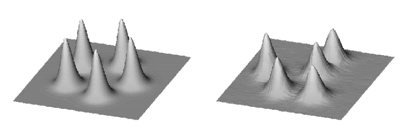
Figure 8: Energy density plots for an initial pentagonal arrangement of 5 vortices. The plots are at times $t=0$ and $t=2500.$

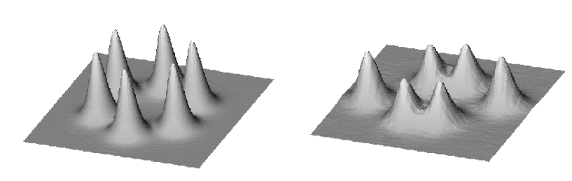
Figure 9: Energy density plots for an initial hexagonal arrangement of 6 vortices. The plots are at times $t=0$ and $t=2000.$

The results of a simulation with five vortices on the vertices of a regular pentagon are shown in Fig. 7(b). The initial vortex positions (white circles) lie on a circle of radius 5, and the lines track the motion for $t\leq 2500.$ It can already be seen from these vortex trajectories that the cyclic $C_{5}$ symmetry gets broken, with one of the vortices already moving closer to the origin than the other four. The black circles denote the vortex positions at time $t=3200,$ and the pentagonal symmetry has obviously been destroyed, with one of the vortices being much further from the origin than the other four. The broken symmetry is most easily visualized through energy density plots. Fig. 8 shows energy density plots at times $t=0$ and $t=2500,$ clearly displaying the broken $C_{5}$ symmetry. Note that the vortices are more localized in the initial conditions than at later times. This is because the initial conditions are formed from critically coupled vortices, but these quickly relax to vortices with a localization appropriate for the chosen coupling $\lambda=0.5.$ The numerical grid extends far beyond the inner portion plotted in these figures, but for clarity we do not display the entire grid.

Further evolution of this configuration suggests that the vortices are tending towards the formation of a pair of axial $N=2$ vortices, plus a single $N=1$ vortex, though our simulations can not be run long enough to confirm the final state. A reasonable expectation is that the vortices combine, at first in pairs, and eventually radiation loss will lead to a final configuration of an axial $5$-vortex.

The instability of the pentagonal arrangement disagrees with the asymptotic moduli space prediction and therefore raises a number of interesting questions as to the source of the disagreement. One possibility is that the asymptotic approximation is correct but that the simulation is not in the asymptotic regime. This would suggest that there may be a critical size for the pentagonal arrangement, with a stability only if the pentagon is above the critical size. This could be investigated by numerically computing the appropriate Kähler form and reduced potential, and then numerically solving an eigenvalue problem to determine if there are any negative modes. This is an interesting project for future investigation.

Another possibility is that there is a stability region in coupling space, so that the pentagon is stable only if $\lambda$ is sufficiently close to critical coupling. It might be possible to investigate this within a moduli space approach by including the deformations of the vortex fields, such as the tiny electric field, which arise away from critical coupling and are not captured by restricting to the critically coupled moduli space. For $\lambda>1$ an appropriate moduli space could be constructed from the unstable manifold of the axial $N=5$ vortex, in a similar way that has been used [2] to study Schrödinger dynamics of two ungauged Ginzburg-Landau vortices.

A final possibility is that the instability is due to a phenomenon that can not be captured by any standard moduli space approach, and the interaction between vortices and radiation plays a crucial role.

The asymptotic moduli space approach predicts that 6 vortices on the vertices of a regular hexagon will be unstable. The results of such an initial arrangement, with the vortices on a circle of radius 5, are presented in Fig. 9. This figure displays energy density plots at times $t=0$ and $t=2000.$ Clearly the cyclic $C_{6}$ symmetry is broken by this time, so this result is in agreement with the instability prediction. Note from the second plot in Fig. 9 that the $C_{6}$ symmetry is broken to a $C_{2}$ symmetry at this stage in the evolution, and again there appears to be a tendency for vortices to form pairs.

In summary, we find that the stability properties of regular polygonal arrangements of vortices is in reasonable agreement with the moduli space prediction, in that we find that an $N$-gon is stable only for small enough values $N<N_{c}.$ However, we conclude that the critical value is $N_{c}=5$ rather than $N_{c}=6,$ and have suggested some approaches that could be used to investigate this discrepancy further.

6 Hyperbolic Vortices

The equations for static critically coupled Ginzburg-Landau vortices on the hyperbolic plane of curvature $-\frac{1}{2}$ are integrable, and this allowed Strachan [12] to calculate a general formula for the Kähler form on the moduli space $M_{N}.$ In this respect hyperbolic vortices are therefore simpler than Euclidean vortices. In this Section we exploit this fact to study the moduli space approximation to Schrödinger-Chern-Simons vortex dynamics on hyperbolic space.

Consider a two-dimensional Riemannian manifold $X,$ with metric

$$ds^{2}=\Omega(x_{1},x_{2})(dx_{1}^{2}+dx_{2}^{2}).$$ (6.1)

Ginzburg-Landau vortices on $X$ are minima of the energy

$$V=\frac{1}{2}\int_{X}\left(\Omega^{-1}B^{2}+\overline{D_{1}\phi}D_{1}\phi+\overline{D_{2}\phi}D_{2}\phi+\frac{\lambda\Omega}{4}(1-\bar{\phi}\phi)^{2}\right)d^{2}x.$$ (6.2)

At the critical coupling $\lambda=1$ the second order equations can again be reduced to first order Bogomolny equations, as in the Euclidean case. Introducing the function $h,$ as in (3.3), then the generalization of the Euclidean equation (3.6) becomes

$$\nabla^{2}h+\Omega-\Omega{\rm e}^{h}=4\pi\sum\limits_{r=1}^{N}\delta(x-X_{r}),$$ (6.3)

where $\nabla^{2}$ is the standard flat space Laplacian and $X_{r}\in X$ are the vortex positions.

In the Poincaré disc model, the metric of the hyperbolic plane with curvature $-\frac{1}{2}$ is

$$ds^{2}=\frac{8}{(1-|z|^{2})^{2}}dzd{\bar{z}}=\Omega~{}dzd{\bar{z}},$$ (6.4)

where $|z|<1$. Setting $h=2g+2\log\frac{1}{2}(1-|z|^{2})$ the equation for $h$ becomes Liouville’s equation with sources

$$\nabla^{2}g-{\rm e}^{2g}=2\pi\sum\limits_{r=1}^{N}\delta(z-Z_{r}),$$ (6.5)

which can be solved exactly. The solution is

$$g=-\log\frac{1}{2}(1-|f|^{2})+\frac{1}{2}\log\left|\frac{df}{dz}\right|^{2},$$ (6.6)

where $f(z)$ is an arbitrary, complex analytic function. With a simple choice of phase the scalar field is given by

$$\phi=\frac{1-|z|^{2}}{1-|f|^{2}}\frac{df}{dz}.$$ (6.7)

Note that $\phi$ vanishes at the zeros of $\frac{df}{dz}$. To ensure that $\phi$ has $N$ zeros, is nonsingular inside the disc $|z|<1$ and is zero on the boundary $|z|=1,$ then the function $f(z)$ needs to have the Blaschke product form

$$f(z)=\prod\limits_{i=1}^{N+1}\left(\frac{z-a_{i}}{1-{\bar{a}}_{i}z}\right),$$ (6.8)

where $|a_{i}|<1$.

Let us now specialize to the case of $N$ vortices on an $N$-gon, including the degenerate case $N=2.$ Such a configuration is described by the holomorphic function

$$f(z)=\frac{z\left(z^{N}-a^{N}\right)}{1-{\bar{a}}^{N}z^{N}}.$$ (6.9)

The positions of the vortices are given by the zeros of the derivative ${df}/{dz}$, and these are the regular $N$-gon vertices given by

$$z=\alpha~{}{\rm e}^{2\pi ik/N}$$ (6.10)

for $k=1,\dots,N$. The parameter $a$ can be expressed in terms of $\alpha$ via $a=\alpha\gamma$ where

$$\gamma^{N}=\frac{\sqrt{\left(1-|\alpha|^{2N}\right)^{2}+4N^{2}|\alpha|^{2N}}-1-|\alpha|^{2N}}{2|\alpha|^{2N}\left(N-1\right)}.$$ (6.11)

Using the results of [12] the Kähler metric on this two-dimensional submanifold of $M_{N}$ can be calculated explicitly and is given by

$$ds^{2}=\frac{4\pi N^{3}|\alpha|^{2N-2}d\alpha~{}d{\bar{\alpha}}}{\left(1-|\alpha|^{2N}\right)^{2}}\left(1+\frac{2N\left(1+|\alpha|^{2N}\right)}{\sqrt{\left(1-|\alpha|^{2N}\right)^{2}+4N^{2}|\alpha|^{2N}}}\right).$$ (6.12)

Note that for $N=2$ this metric becomes the one derived by Strachan [12], which he used to study the relativistic dynamics of two hyperbolic vortices.

Given the metric (6.12) the Kähler form $\omega$ can simply be read off. Let $\alpha=r{\rm e}^{i\theta},$ then

$$\omega=f(r)dr\wedge d\theta,$$ (6.13)

where

$$f(r)=\frac{2\pi N^{3}r^{2N-1}}{\left(1-r^{2N}\right)^{2}}\left(1+\frac{2N\left(1+r^{2N}\right)}{\sqrt{\left(1-r^{2N}\right)^{2}+4N^{2}r^{2N}}}\right).$$ (6.14)

Now that we have the Kähler form, all that we require to study Schrödinger-Chern-Simons vortex dynamics is the reduced potential. This is given by the expression

$$V_{\mbox{red}}=N\pi+\frac{\lambda-1}{8}\int_{X}(1-|\phi|^{2})^{2}~{}\Omega~{}d^{2}x,$$ (6.15)

where the explicit solution for $\phi$ is known from above using (6.7) and (6.9). It can be shown that this reduced potential depends only on $|\alpha|.$ Unfortunately this integral over the hyperbolic plane can not be performed explicitly (except for the special value $\alpha=0$) even in the case $N=2.$ The angular part of the integral can be calculated explicitly but the radial integration must then be computed numerically.

With the Kähler form and reduced potential given above the moduli space dynamics reduces to the equations of motion ${\dot{r}}=0$ and

$$2f(r){\dot{\theta}}=-\frac{dV_{\mbox{red}}}{dr}.$$ (6.16)

Thus, as in the Euclidean case, the configuration rigidly rotates with no change in size and with constant angular velocity ${\dot{\theta}}.$ The period is

$$T=\left|\frac{4\pi f(r)}{dV_{\mbox{red}}/dr}\right|.$$ (6.17)

In order to compare the period calculation in hyperbolic space to the earlier results in Euclidean space, we need to calculate the proper distance. From the Poincaré disc coordinate $z=|z|e^{i\chi}$ we make the transformation $\rho=2\sqrt{2}\tanh^{-1}(|z|)$ so that the hyperbolic metric becomes

$$ds^{2}=d\rho^{2}+2\sinh^{2}\left(\frac{\rho}{\sqrt{2}}\right)d\chi^{2}.$$ (6.18)

Thus $\rho$ should be equated with the radial distance in Euclidean space.

In Fig. 10 we plot (dashed curve) the scaled period $T|\lambda-1|$ as a function of the separation $s=2\rho$ for the two-vortex case ie. $N=2.$ For comparison we also reproduce the earlier Euclidean result (solid curve). The Euclidean and hyperbolic results are qualitatively similar. Both periods are monotonically increasing functions of the separation and tend to finite non-zero limits as the separation tends to zero. The simplifications of hyperbolic space allow the period to be calculated accurately all the way down to zero separation, and this value appears similar to the one extrapolated from the Euclidean data. Note that it is not expected that the Euclidean and hyperbolic periods agree at zero separation since the vortices are extended objects, so even when both vortices are located at the origin they still feel the curvature of hyperbolic space.

The period for an $N$-gon arrangement of hyperbolic vortices can also be calculated using the above methods and the results are qualitatively similar to the 2-vortex case. The period at zero separation is not very sensitive to the value of $N$ but does slightly decrease as $N$ increases.

Figure 10: The scaled period $T|\lambda-1|$ against separation $s$ for two vortices in Euclidean space (solid curve) and hyperbolic space (dashed curve).

The similarity between the moduli space results for Euclidean and hyperbolic space suggests that it would be interesting to investigate the stability of polygonal arrangements of hyperbolic vortices. Although this is still not an easy exercise it is substantially simpler than the Euclidean case, since the exact static vortex solutions are available at critical coupling.

7 Conclusions

In this paper we have studied the dynamics of vortices in Manton’s Schrödinger-Chern-Simons model, and compared the results of full field simulations with predictions from the moduli space approximation. We found that there is a good agreement for couplings extremely close to the critical coupling, but away from this value there are significant qualitative differences, which we attribute to radiation effects which are not captured by the moduli space approach. This is of physical relevance since real superconductors are generally not close to the Type I/Type II transition.

A novel suggestion might be to try and modify the non-dissipative moduli space dynamics to a new dissipative dynamics on the moduli space that would capture the energy loss effects. The Schrödinger-Chern-Simons flow is orthogonal, in a rigourous mathematical sense, to the gradient flow of the Ginzburg-Landau energy, so a flow which contains both components should certainly reproduce the qualitative features that we have found. However, it is not clear how to derive such a flow from the field theory, but it would seem a worthwhile avenue for further investigation.

In the Schrödinger dynamics of two ungauged Ginzburg-Landau vortices it has been shown analytically that two vortices radiate while rotating around each other and the asymptotic rate at which they radiate has been derived [7]. In the ungauged system the coupling constant plays no role. Motivated by the numerical results we have presented here, it would be interesting if the methods used in [7] could be applied to the Schrödinger-Chern-Simons model and similar results derived, including the coupling constant dependence. This is another interesting topic for future work, though the inclusion of gauge fields, and in particular the requirement of working with gauge independent quantities, appears to make the problem significantly more complicated than in the ungauged situation.

Finally, we have demonstrated that, at least within the moduli space approximation, the qualitative features of Euclidean vortices appear to be shared by hyperbolic vortices. This opens up the possibility of future studies on the stability properties of symmetric arrangements of hyperbolic vortices, for arbitrary separations, exploiting the fact that hyperbolic vortices are simpler to study due to the existence of exact static solutions at critical coupling.

Appendix: The linearized field equations

In this appendix, we discuss the linearized field equations and their plane wave solutions. It is convenient to work in a gauge such that $\phi$ is real. Setting $\phi=1+\sigma$, we can linearize around the vacuum $\phi=1$ and $a_{\mu}=0$, by expanding the field equations (2.6), (2.7) and (2.8) in $\sigma$ and $a_{\mu}$ to linear order. First, we eliminate $a_{0}$ using the linearized real part of (2.6)

$$2a_{0}=-\nabla^{2}\sigma+\lambda\sigma,$$ (A.1)

where $\nabla^{2}=\partial_{1}^{2}+\partial_{2}^{2}.$ Then we replace $\sigma$ using the linearized Gauss equation

$$\sigma=-B.$$ (A.2)

Finally, from (2.7) we obtain

$$\left(\begin{array}[]{c}2{\dot{a}_{1}}\\ 2{\dot{a}_{2}}\end{array}\right)=\left(\begin{array}[]{cc}(1+\lambda-\nabla^{2})\partial_{1}\partial_{2}&1-(1+\lambda-\nabla^{2})\partial_{1}^{2}\\ -1+(1+\lambda-\nabla^{2})\partial_{2}^{2}&-(1+\lambda-\nabla^{2})\partial_{1}\partial_{2}\end{array}\right)\left(\begin{array}[]{c}a_{1}\\ a_{2}\end{array}\right).$$ (A.3)

Note that the determinant of the symbol of the differential operator in (A.3) vanishes. In order to find plane wave solutions we make the ansatz $a_{i}=A_{i}\exp(i({\bf k}\cdot{\bf x}-\omega t))$. This results in a linear homogeneous matrix equation which has nontrival solutions only if the determinant vanishes, namely,

$$-4\omega^{2}+k^{4}+(1+\lambda)k^{2}+1=0,$$ (A.4)

where $k^{2}=k_{1}^{2}+k_{2}^{2}$. This gives rise to the nonlinear dispersion relation

$$\omega=\frac{1}{2}\sqrt{k^{4}+(1+\lambda)k^{2}+1},$$ (A.5)

which for critical coupling $\lambda=1$ reduces to

$$\omega=\frac{1}{2}(k^{2}+1).$$ (A.6)

For general $\lambda$ the corresponding linearized solution is given by

$$\left(\begin{array}[]{c}a_{1}\\ a_{2}\end{array}\right)=\alpha\left(\begin{array}[]{c}\cos\left({\bf k}\cdot{\bf x}-\omega t+\delta\right)\\ \frac{k_{1}k_{2}(k^{2}+1+\lambda)}{k_{1}^{2}(k^{2}+1+\lambda)+1}\cos\left({\bf k}\cdot{\bf x}-\omega t+\delta\right)+\frac{\sqrt{1+(1+\lambda)k^{2}+k^{4}}}{k_{1}^{2}(k^{2}+1+\lambda)+1}\sin\left({\bf k}\cdot{\bf x}-\omega t+\delta\right)\end{array}\right),$$ (A.7)

where $\alpha$ and $\delta$ are constants. This shows that the plane wave solutions are elliptically polarised, as can be seen for example from the fact that the modulus of the vector (A.7) is not time independent.

References

- [1] I. J. R. Aitchison, P. Ao, D. L. Thouless and X.-M. Zhu, Effective Lagrangians for BCS superconductors at , Phys. Rev. B51, 6531 (1995).
- [2] O. Lange and B. J. Schroers, Unstable manifolds and Schrödinger dynamics of Ginzburg-Landau vortices, Nonlinearity 15, 1471 (2002).
- [3] N. S. Manton, An effective Lagrangian for solitons, Nucl. Phys. B150, 397 (1979).
- [4] N. S. Manton, First order vortex dynamics, Ann. Phys. 256, 114 (1997).
- [5] N. S. Manton and J. M. Speight, Asymptotic interactions of critically coupled vortices, Commun. Math. Phys. 236, 535 (2003).
- [6] N. S. Manton and P. M. Sutcliffe, Topological Solitons, Cambridge University Press (2004).
- [7] Yu. N. Ovchinnikov and I. M. Sigal, The Ginzburg-Landau equation III. Vortex dynamics, Nonlinearity 11, 1277 (1998); Long-time behaviour of Ginzburg-Landau vortices, ibid 11, 1295 (1998); Dynamics of localized structures, Physica A261, 143 (1998).
- [8] N. M. Romão and J. M. Speight, Slow Schrödinger dynamics of gauged vortices, Nonlinearity 17, 1337 (2004).
- [9] T. M. Samols, Vortex scattering, Commun. Math. Phys. 145, 149 (1992).
- [10] P. A. Shah, Scattering of vortices at near-critical coupling Nucl.Phys. B429, 259 (1994).
- [11] J. M. Speight, Static intervortex forces, Phys. Rev. D55, 3830 (1997).
- [12] I. A. B. Strachan, Low-velocity scattering of vortices in a modified abelian Higgs model, J. Math. Phys. 33, 102 (1992).
- [13] D. Stuart, Dynamics of abelian Higgs vortices in the near Bogomolny regime, Commun. Math. Phys. 159, 51 (1994).
- [14] P. M. Sutcliffe, The interaction of Skyrme-like lumps in (2+1) dimensions, Nonlinearity 4, 1109 (1991).
- [15] C. H. Taubes, Arbitrary -vortex solutions to the first order Ginzburg-Landau equations, Commun. Math. Phys. 72, 277 (1980).