The properties of attractors of canalyzing random Boolean networks

Abstract

We study critical random Boolean networks with two inputs per node that contain only canalyzing functions. We present a phenomenological theory that explains how a frozen core of nodes that are frozen on all attractors arises. This theory leads to an intuitive understanding of the system’s dynamics as it demonstrates the analogy between standard random Boolean networks and networks with canalyzing functions only. It reproduces correctly the scaling of the number of nonfrozen nodes with system size. We then investigate numerically attractor lengths and numbers, and explain the findings in terms of the properties of relevant components. In particular we show that canalyzing networks can contain very long attractors, albeit they occur less often than in standard networks.

1 Introduction

Random Boolean networks are often used as generic models for the dynamics of complex systems of interacting entities, such as social and economic networks, neural networks, and gene or protein interaction networks Kauffman et al. (2003). The simplest and most widely studied of these models was introduced in 1969 by Kauffman Kauffman (1969) as a model for gene regulation. The system consists of $N$ nodes, each of which receives input from $K$ randomly chosen other nodes. The network is updated synchronously, the state of a node at time step $t$ being a Boolean function of the states of the $K$ input nodes at the previous time step, $t-1$. The Boolean update functions are randomly assigned to every node in the network, and together with the connectivity pattern they define the realization of the network. For any initial condition, the network eventually settles on a periodic attractor. Of special interest are critical networks, which lie at the boundary between a frozen phase and a chaotic phase Derrida and Pomeau (1986); Derrida and Stauffer (1986); Moreira and Amaral (2005). In the frozen phase, a perturbation at one node propagates during one time step on an average to less than one node, and the attractor lengths remain finite in the limit $N\to\infty$. In the chaotic phase, the difference between two almost identical states increases exponentially fast, because a perturbation propagates on an average to more than one node during one time step Aldana-Gonzalez et al. (May 2003).

Critical networks with $K=2$ inputs per node have been studied by a variety of authors. A $K=2$ network is critical if frozen and reversible update functions are chosen with equal probability. The remaining update functions are canalyzing, i.e., one input can fix the output of a node, irrespective of the value of the second input. Table 1 shows the 16 update functions of $K=2$ networks.

In	$\mathcal{F}$		${\mathcal{C}}_{1}$				${\mathcal{C}}_{2}$								$\mathcal{R}$
00	1	0	0	1	0	1	1	0	0	0	0	1	1	1	1	0
01	1	0	0	1	1	0	0	1	0	0	1	0	1	1	0	1
10	1	0	1	0	0	1	0	0	1	0	1	1	0	1	0	1
11	1	0	1	0	1	0	0	0	0	1	1	1	1	0	1	0

Table 1: The 16 update functions for nodes with two inputs. The first column lists the 4 possible states of the two inputs, the other columns represent one update function each, falling into the classes frozen ($\mathcal{F}$), canalyzing (${\mathcal{C}}_{1}$ and ${\mathcal{C}}_{2}$) and reversible ($\mathcal{R}$).

Critical networks that contain a nonvanishing proportion of frozen and reversible update functions are in the meantime relatively well understood, see Bilke and Sjunnesson (2002); Socolar and Kauffman (2003); Samuelsson and Troein (2003); Gershenson (2004); Klemm and Bornholdt (2005); Drossel (2005); Kaufman et al. (2005). They contain three classes of nodes, which behave differently on attractors. First, there are nodes that are frozen on the same value on every attractor. Such nodes give a constant input to other nodes and are otherwise irrelevant. They form the frozen core of the network. Second, there are nodes without outputs and nodes whose outputs go only to irrelevant nodes. Though they may fluctuate, they are also classified as irrelevant since they act only as slaves to the nodes determining the attractor period. Third, the relevant nodes are the nodes whose state is not constant and that control at least one relevant node. These nodes determine completely the number and period of attractors. If only these nodes and the links between them are considered, these nodes form loops with possibly additional links and chains of relevant nodes within and between loops. We call a set of relevant nodes that are connected in this way a relevant component. The nonfrozen nodes that are not relevant sit on trees rooted in the relevant components. In Socolar and Kauffman (2003), it was found that the number of nonfrozen nodes scales in the limit $N\to\infty$ as $N^{2/3}$ and the number of relevant nodes as $N^{1/3}$. This result was confirmed by an analytical calculation in Kaufman et al. (2005), where it was additionally shown that the number of nonfrozen nodes with two nonfrozen inputs scales as $N^{1/3}$, and that the number of relevant nodes with two relevant inputs remains finite in the limit $N\to\infty$. The mean number of relevant components was found to be proportional to $\ln N$, and all but the largest relevant components are simple loops.

Canalyzing networks share many features of other critical networks. Thus, the calculation by Samuelsson and Troein Samuelsson and Troein (2003) of the number of attractors can be generalized to canalyzing networks Drossel (2005), implying that canalyzing networks also have of the order of $N^{2/3}$ nonfrozen nodes and at most $N^{1/3}$ nonfrozen nodes with two relevant inputs, and that the mean attractor number increases faster than any power law with the network size. Whether the nonfrozen nodes are the same on all attractors in canalyzing networks (as is the case of networks containing frozen update functions), can not be decided from previous work. In particular, the detailed results of Kaufman et al. (2005) can only be derived if there are nodes with frozen functions. For these reasons, a separate study of canalyzing networks is needed. It is the main aim of this paper to show how the attractors and the frozen nodes arise in canalyzing networks. We will see that canalyzing networks also have a frozen core, which means that most frozen nodes are the same on all attractors. It follows then that all results of Kaufman et al. (2005) about the relevant part of the network can be applied also to canalyzing networks. We will also put an end to the long-standing belief that canalyzing networks have less and shorter attractors. These features were argued to make canalyzing networks biologically more relevant Kauffman et al. (2003).

Let us therefore focus on $K=2$ networks that contain only $\mathcal{C}_{2}$ functions. These functions take one value (0 or 1) three times and the other one once. This means that each of the two inputs can fix the output of the function irrespective of the other input. For instance, the output of the first $\mathcal{C}_{2}$ function shown in Table 1 must be 0 if the first input is 1, irrespective of the second input. It must also be 0 if the second input is 1, irrespective of the first input. Each of the 8 $\mathcal{C}_{2}$ functions is chosen with equal probability in our simulations. We will compare our results for $\mathcal{C}_{2}$ networks with those of standard random Boolean networks (RBNs), where all 16 update functions have the same weight. Part of our results will also be compared to those of $\mathcal{C}_{1}$ networks, where the update functions are chosen only from the $\mathcal{C}_{1}$ class. The $\mathcal{C}_{1}$ networks can be trivially mapped on critical $K=1$ networks by removing the link to the input to which the node does not respond. These networks have no frozen core. They have of the order of $\sqrt{N}$ relevant nodes, arranged in $\sim\ln N$ simple loops (see Drossel et al. (2005)), with the largest loop length being of the order $\sqrt{N}$. The other nodes sit on trees rooted in these loops.

In the next Section, we study numerically the frozen nodes in order to find out if the same nodes are frozen on all attractors of $\mathcal{C}_{2}$ networks. In Section 3, we explain the results of the numerical simulations using phenomenological arguments and analytical calculations. In Section 4, we study the number and length of attractors of $\mathcal{C}_{2}$ networks and compare the results to those of other network types. Finally we summarize and discuss our results in the last Section.

2 The frozen core

From a generalization of the work of Samuelsson and Troein Samuelsson and Troein (2003) to all critical $K=2$ random Boolean networks Drossel (2005), we know that for canalyzing networks the number of nonfrozen nodes scales for large network size in the same way as for RBNs, i.e., with $N^{2/3}$. In RBNs, the nodes frozen on all attractors (i.e., the nodes belonging to the frozen core) can be identified by starting with the nodes with frozen update functions and by iteratively determining nodes that become frozen because of frozen inputs, see Kaufman et al. (2005). In canalyzing networks there are no frozen functions to start with, and this method cannot be applied. It therefore arises the question whether canalyzing networks have a frozen core at all, or whether different attractors have different nonfrozen nodes. In the following, we will answer this question using computer simulations.

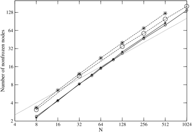
Figure 1: Mean number of nonfrozen nodes for canalyzing $\mathcal{C}_{2}$ networks (stars) and RBNs (circles). Solid lines connect the data points for $N-N_{f}^{(a)}$ (mean number of nonfrozen nodes per attractor), dashed lines the data points for $N-N_{f}^{(n)}$ (mean number of nodes that are nonfrozen at least on one found attractor). The dotted line is a power law $N^{2/3}$. Different attractors are counted only once, without considering their basins of attraction. We have considered 1000 initial states per network, averaged over 2000 networks.

In Fig. 1 we show the average number $N_{f}^{(a)}$ of frozen nodes per attractor, both for canalyzing networks and for RBNs. We actually plot the difference $(N-N_{f}^{(a)})$ as a function of $N$ in order to better see the asymptotic behavior. The other two curves show the difference $(N-N_{f}^{(n)})$, where $N_{f}^{(n)}$ is the number of nodes frozen on all attractors found in the simulation of a network. The technical details can be found in the caption to the figure.

One can clearly see the similarity of the results for the mean number of nonfrozen nodes per attractor $(N-N_{f}^{(a)})$ for canalyzing networks and for RBN, in agreement with Samuelsson and Troein (2003); Drossel (2005). The expected power law $N^{2/3}$ is not yet reached for the system sizes used in the simulation and is only approached slowly with increasing $N$. The number of nonfrozen nodes in the simulations was only of the order of 100 for the largest simulated networks, which is yet too small to see the asymptotic behavior. (And the number of relevant nodes, which increases as $N^{1/3}$, is only of the order $10$ for the largest simulated networks.)

Our results for $(N-N_{f}^{(n)})$ suggest that canalyzing networks have a frozen core and of the order of $N^{2/3}$ nonfrozen nodes, because the curves for $(N-N_{f}^{(n)})$ differ only by a constant factor from those for $(N-N_{f}^{(a)})$ for both network types. Furthermore, there are of the order of $N^{2/3}$ nodes that are frozen only on part of the attractors. The factor between the two curves is larger for canalyzing networks than for RBN.

In the following, we will explain the reason for the constant factor between the curves for $(N-N_{f}^{(a)})$ and $(N-N_{f}^{(n)})$. Since this point has not yet been discussed for RBNs, we will consider both RBNs and canalyzing networks. The explanation of the origin of the frozen core in canalyzing networks will be postponed until the next Section.

The difference between the curves for $(N-N_{f}^{(a)})$ and $(N-N_{f}^{(n)})$ is due to those nodes that are frozen on some attractors, but not on all attractors. These nodes do not belong to the frozen core, and they are therefore relevant nodes or sit on nonfrozen trees that are rooted in relevant components. In Section 1, we have mentioned that most relevant components consist of simple loops, and that only a few large components are more complex and contain relevant nodes that have two relevant inputs. Clearly, since the dynamics of the nonfrozen nodes in the trees is determined by the dynamics of the relevant nodes, all nodes of a relevant component and the nonfrozen trees rooted in it undergo a cycle of the same period (when the attractor has been reached), which is determined by the initial state of the relevant nodes of that component. If this cycle has period one, all nodes of this component are frozen on this attractor. We therefore have to show that a finite fraction of all nonfrozen nodes are on cycles of length 1 on a finite fraction of all attractors. This would lead to a constant factor between the curves for $(N-N_{f}^{(a)})$ and $(N-N_{f}^{(n)})$.

Let us first consider relevant components that are simple loops, and their nonfrozen trees. The mean number of relevant loops of length $l$ is $1/l$ for all $l$ up to a cutoff $l_{c}\sim N^{1/3}$. The mean size of a tree rooted in a relevant node is $N^{1/3}$. The largest of these components consists therefore of the order of $N^{2/3}$ nodes (including the nonfrozen trees), and if such a component reaches a fixed point attractor with nonzero probability, we have explained the factor between the two curves. A relevant loop of length $l$ has either two fixed points (if the loop is “even”, i.e. if the state of a node is repeated after $l$ time steps) or none (if the loop is “odd”, i.e. the state of a node is inverted after $l$ time steps). Each case occurs with probability 1/2. The number of attractors of a component with a loop of length $l$, however, increases exponentially with $l$, and for this reason only a vanishing proportion of attractors of components of a size of the order $l_{c}$ are fixed points in the limit of large $N$.

Next, we consider complex relevant components. In contrast to simple loops, where each initial state is part of a periodic cycle in state space, more complex components can have fixed points that are true attractors, i.e. that are reached from a nonvanishing proportion of initial states (but not from all initial states). One example of such a component in RBNs was discussed in Kaufman and Drossel (2005). It is a loop with an additional chain of nodes within the loop, such that there is one node that has two relevant inputs. From Kaufman et al. (2005), we know that this component occurs with nonvanishing probability in an RBN. In the case that the update function of the node with two inputs is 0 only if both inputs are 0 and that the two numbers of nodes on the two subloops have a common divisor greater $1$, all apart from a finite number of initial conditions end up on the same fixed point. The existence of such components does not only explain the multiplicative factor between the curves for $(N-N_{f}^{(n)})$ and $(N-N_{f}^{(a)})$, but it explains also why this factor is larger for $\mathcal{C}_{2}$ networks than for RBNs. The probability that an update function as in the above example is chosen at the relevant node with two inputs is larger for canalyzing networks.

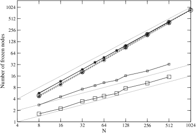
Figure 2: Number of frozen nodes for $K=1$ networks. Large squares: $N_{f}^{(n)}$; small squares: $N_{f}^{(a)}$. For comparison, the corresponding curves for RBNs and $\mathcal{C}_{2}$ networks are also shown, the data is taken from Fig. 1. The dotted lines correspond to the power laws $N,\;\sqrt{N}$ and $\sqrt{N}/2$.

We conclude this Section by comparing $\mathcal{C}_{2}$ networks with $\mathcal{C}_{1}$ networks, which are canalyzing networks, but with update functions of the $\mathcal{C}_{1}$ class. Our simulation results for $N_{f}^{(a)}$ and $N_{f}^{(n)}$ are shown in Fig. 2. Both curves increase for $\mathcal{C}_{1}$ networks as $\sqrt{N}$. Asymptotically, $N_{f}^{(n)}$ is of the order $\sqrt{N}/2$, since only even loops of length $1$ can be frozen on all attractors, while the average tree size is of the order of $\sqrt{N}$. To calculate $N_{f}^{(a)}$ we note that only even loops of length $l$ have (two) fixed points, and that they do not reach these fixed points for $2^{l}-2$ initial conditions. The contribution to the average number of frozen nodes per attractor from simple loops of length $l$ is then $1/l\cdot 1/2\cdot 2l/2^{l}\cdot\sqrt{N}$, where we again take the probability of an even loop $1/2$ and the average size of a tree of the order of $\sqrt{N}$ into account. Summing over $l$ leads to $N_{f}^{(a)}\to\sqrt{N}$. We conclude that, differently from $\mathcal{C}_{2}$ networks, the ratio $(N-N_{f}^{(n)})/(N-N_{f}^{(a)})$ approaches 1 asymptotically. As we have learned, the reason for a larger factor between the two curves for RBNs and $\mathcal{C}_{2}$ networks is the existence of complex relevant components. In $\mathcal{C}_{1}$ networks all relevant components are simple loops.

3 Self-freezing loops

In this Section, we want to explain how the frozen core arises in $\mathcal{C}_{2}$ networks and find some of its properties. We also estimate its size by means of analytical arguments. The results are in agreement with Samuelsson and Troein (2003); Drossel (2005), confirming our intuitive understanding of the origin of the frozen core.

Since a $\mathcal{C}_{2}$ network has no nodes with a frozen function, the frozen core cannot be formed starting from single frozen nodes. Instead, there must exist groups of nodes that fix each other’s value and do not respond to changes in nodes outside this group. Let us consider the simplest example of such a group, namely a loop where each node canalyzes (fixes) the state of its successor once it settles on its majority bit (the one occuring 3 times in its update function table). We call such loops self-freezing loops. In the following, we first discuss these self-freezing loops, before discussing how a frozen core that contains almost all nodes can be formed starting from these loops.

If all nodes of a self-freezing loop are on their majority bits, it stays frozen forever. Starting from an arbitrary initial state, the number of nodes of a self-freezing loop on majority bits cannot decrease with time, since each such node drives its successor to its majority bit. It remains constant only in the unlikely case that all inputs from outside the loop to the nodes of the loop are fixed on the noncanalyzing value. We can therefore assume that self-freezing loops are usually frozen on all attractors, at least if the loops are large. As we will see, most nodes that are part of self-freezing loops sit in loops with a size of the order of $N^{1/3}$.

The number of nodes on self-freezing loops can be estimated as follows. The probability that a given node constitutes a self-freezing loop of length $1$ is $1/N$ for a network with $N$ nodes. It is the product of the probability $2/N$ that the node is self-connected and the probability $1/2$ that the node is canalyzed by its own majority bit. There is thus on average one self-freezing loop of length $1$ per network. With the same line of reasoning, the average number of self-freezing loops of length $2$ per network is obtained to be $\binom{N}{2}\left(\frac{2}{N}\right)^{2}\left(\frac{1}{2}\right)^{2}\approx\frac{1}{2}$. For the self-freezing loops of length $l>2$ one has to take into account an additional factor, corresponding to the number of ways to construct a directed loop out of $l$ nodes. The number of self-freezing loops of length $l$ per network is found to be $1/l$. The overall number of nodes on self-freezing loops $f_{0}$ is then

$$f_{0}=\Sigma_{l=1}^{l_{c}}\frac{1}{l}l=l_{c},$$ (1)

$l_{c}$ being the cutoff in loop length. This simple probabilistic considerations applies if $l_{c}$ is much smaller than $N$.

We can obtain a confirmation of this estimation and a result for the value of $l_{c}$ by mapping the problem of finding a self-freezing loop in a $\mathcal{C}_{2}$ network onto the problem of finding the relevant nodes sitting on relevant loops in a critical network that contains no canalyzing functions at all, but only $\mathcal{R}$ and $\mathcal{F}$ functions. Whether a randomly chosen node in such a network is part of a relevant loop is determined by the following algorithm. Consider the two inputs of this node. With probability 1/4, both inputs have a frozen update function, and the node is not relevant. With probability 1/2, one input has a frozen update function and the other one a reversible one. In this case we draw a link to this reversible input node and thus mark it for investigation of its two inputs in the next step. With probability 1/4, both inputs have reversible update functions, and we draw links to both of them. We iterate this procedure, choosing at each step the two inputs of a node at random from all nodes, and drawing links to those inputs that do not have frozen update function. The procedure continues until we either find a connection back to the original node (in which case it is relevant), or until no more links can be drawn (in which case the original node is not part of a relevant loop). From the results of our article Kaufman et al. (2005), we know that there is a mean number of $1/l$ relevant loops of size $l$ in such a network, and that the cutoff in the size of relevant components scales as $N^{1/3}$.

Now, we turn to the procedure of finding self-freezing loops in $\mathcal{C}_{2}$ networks and show that it is identical to the procedure just described. We start with a randomly chosen node and determine whether it is part of a self-freezing loop. Consider the two inputs of this node. With probability 1/4, the majority bit of neither input canalyzes the chosen node, and the node is not on a self-freezing loop. With probability 1/2, the majority bit of one input does not canalyze the chosen node, and the majority bit of the other input canalyzes it. Let us draw a link to this input node and consider its two inputs in the next step. With probability 1/4, the majority bits of both inputs canalyze the chosen node, and we draw links to both of them. We iterate this procedure, choosing at each step the two inputs of a node at random from all nodes, and drawing links to those inputs, whose majority bits canalyze the node. The procedure continues until we either find a connection back to the original node (in which case it is part of a self-freezing loop), or until no more links can be drawn (in which case the original node is not part of a self-freezing loop). The analogy of the two procedures is obvious, and we conclude $l_{c}\sim N^{1/3}$ and $f_{0}\sim N^{1/3}$.

Obviously, nodes depending on or canalyzed by the frozen nodes of the self-freezing loops freeze also, and such nodes may lead to the freezing of further nodes, etc. We introduce a dynamical process in order to determine the total number of nodes that become frozen because of the self-freezing loops. We denote with $f$ the number of nodes that have already become frozen during the process, and the influence of which on other nodes has yet to be determined. $n_{1}$ is the number of nodes for which we already know that one of their inputs is frozen but does not canalyze them, and $n_{2}$ is the number of nodes for which no frozen input was yet identified. Initially, $n_{1}=0$, $f=f_{0}$, $n_{2}=N-f_{0}$ and $n\equiv f+n_{1}+n_{2}=N$. We answer for one of the frozen nodes at a time the question whose input it is. It is an input to any of the $n_{2}$ nodes with probability $2/n$. With equal probability $1/2$, the node either becomes frozen by this input, or it becomes a non-frozen node with effectively one input (called a $\mathcal{C}_{1}$ node in the following). If a node with one input chooses the given frozen node as input (that happens with probability $1/n$), it becomes frozen. At each step, the connected frozen node is being excluded from further consideration. The dynamical process stops when all the nodes are frozen (which is improbable) or when there are no more frozen nodes the influence of which on other nodes has not yet been determined. The dynamical equations for this process are

$$\Delta f =-1+\xi_{1}+\xi_{2}\,,$$

$$\Delta n_{1} =(n_{2}-n_{1})/n\,,$$ (2)

$$\Delta n_{2} =-2n_{2}/n\,.$$

The stochastic Poisson distributed noise terms $\xi_{1}$ and $\xi_{2}$ with the mean values $n_{1}/n$ and $n_{2}/n$ respectively have to be taken into account in the equation for $f$, since $f$ becomes small during the process, so that the noise becomes important, compare Kaufman et al. (2005). The sum $n=f+n_{1}+n_{2}$ decreases by 1 in each step.

Simulations of this process show that the total number of nodes that are frozen because of the self-freezing loops is around $\sim N^{0.8}$, and that the number or nodes that are not fixed by the self-freezing loops is of the order of $N$. The number of nodes frozen because of the self-freezing loops is not large enough to explain the simulation data of the previous Section. We therefore have to find a mechanism that generates more frozen nodes. This is found by extending the definition of self-freezing loops. We have just seen that nodes with one nonfrozen input appear as we identify frozen nodes. Among the nodes that are not frozen by the original self-freezing loops, there are new types of self-freezing loops that contain chains of nodes with one nonfrozen input between $\mathcal{C}_{2}$ nodes. If a chain between two $\mathcal{C}_{2}$ nodes as a whole inverts its input, the inverted majority bit of the first $\mathcal{C}_{2}$ node has to canalyze the second $\mathcal{C}_{2}$ node. As with original self-freezing loops we can claim that the generalized self-freezing loops are usually frozen on attractors. At the end of the process described by (3), the generalized self-freezing loops need to be found. The only effect of nodes with $\mathcal{C}_{1}$ functions in such loops is to delay the signal propagation between two adjacent $\mathcal{C}_{2}$ nodes. The remaining $n_{2}$ nodes with $\mathcal{C}_{2}$ functions can therefore be considered as an effective $\mathcal{C}_{2}$ network, which leads to ${n_{2}}^{1/3}$ nodes on generalized self-freezing loops with similar loop size statistics as discussed above. The independence of the second search for self-freezing loops from the first one is due to the large enough number $n_{1}$ at the end of the process (3). This $n_{1}$ ensures that typical self-freezing loop in the effective $\mathcal{C}_{2}$ network have insertions of $\mathcal{C}_{1}$ chains.

With the new self-freezing loops we again run the dynamical process of type (3). We can even take over the values of $n_{1}$, $n_{2}$ and $n=n_{1}+n_{2}$ at the end of the first process, since ${n_{2}}^{1/3}$ frozen nodes are negligible in comparison with $n_{2}$. Therefore the two equations

$$\Delta n_{1} =(n_{2}-n_{1})/n\,,$$

$$\Delta n_{2} =-2n_{2}/n\,.$$ (3)

apply to both processes together. The equation for $n$ is $\Delta n=-1$, as before. The solution of these equations is obtained by going to differential equations for $dn_{1}/dn$ and $dn_{2}/dn$, which have the solution

$$n_{2}=\frac{n^{2}}{N}\,,$$ (4)

$$n_{1}=n-\frac{n^{2}}{N}\,.$$ (5)

In the same way, at the end of the second process we have again an effective $\mathcal{C}_{2}$ network, with chains containing newly generated $\mathcal{C}_{1}$ nodes. The number of remaining $\mathcal{C}_{1}$ nodes increases in the second process, the number of $\mathcal{C}_{2}$ nodes decreases, thus leading to an increasing weight of $\mathcal{C}_{1}$ nodes in the nonfrozen network. Equations (3) are now applied to a third process, similar to the first two.

The repeated process of identifying generalized self-freezing loops and the nodes frozen by them breaks down when the remaining nonfrozen nodes cannot be considered as an effective $\mathcal{C}_{2}$ network any more. This happens when the proportion $n_{2}/n$ of $\mathcal{C}_{2}$ nodes becomes of the order $\sim 1/\sqrt{n}$. Then, in the process of building a self-freezing loop, there occur $\mathcal{C}_{1}$ chains of an average length of the order $\sim\sqrt{n}$ between $\mathcal{C}_{2}$ nodes. Now, the probability to attach a $\mathcal{C}_{2}$ input at the end of the chain is of the same order of magnitude $1/\sqrt{n}$ as the probability to attach some node of this chain at the end of the chain, in which case the chain becomes a loop, and the assembly of self-freezing loop becomes improbable.

Let us denote by $N_{nf}$ the average number of nonfrozen nodes in $\mathcal{C}_{2}$ networks and by $N_{2}$ the average number of nonfrozen nodes with two inputs. $N_{1}=N_{nf}-N_{2}$ is then the average number of nodes with one nonfrozen input. The breakdown condition for the iterated process becomes then $N_{2}\sim\sqrt{N_{nf}}$. Inserting the condition $n_{2}\sim\sqrt{n}$ in the solution (4), we obtain

$$N_{nf} \sim N^{2/3}\,,$$ (6)

$$N_{2} \sim N^{1/3}\,.$$

This is in agreement with the results of Samuelsson and Troein (2003); Drossel (2005) and confirms our intuitive understanding of the frozen core. The frozen core consists of self-freezing loops, which arise in the interated process described in this Section. The number of nonfrozen nodes is of the order $N^{2/3}$, with only $N^{1/3}$ nonfrozen nodes having 2 nonfrozen inputs. The properties of the nonfrozen part of the network are therefore the same as those of RBNs, and we can take over the results obtained for the nonfrozen part of RBNs. In particular, we can conclude that the number of relevant nodes scales as $N^{1/3}$, with only a finite number of them having two nonfrozen inputs, and with most relevant components being simple loops.

The considerations of this Section can be repeated without change also for mixed $\mathcal{C}_{1}$ and $\mathcal{C}_{2}$ critical Boolean networks, consisting of nonfrozen nodes with one input and of nodes with two inputs having update functions of class $\mathcal{C}_{2}$ , provided that the number of nodes with two inputs is larger than $\sqrt{N}$ (otherwise we are left with a $\mathcal{C}_{1}$ network). Therefore, all the results valid for $\mathcal{C}_{2}$ networks apply also to mixed $\mathcal{C}_{1}$ /$\mathcal{C}_{2}$ networks.

4 Number and length of attractors

We also performed simulations to obtain statistical properties of the attractors of $\mathcal{C}_{2}$ networks in comparison to RBNs and $\mathcal{C}_{1}$ networks. With the intuitive understanding developed in the previous Section we can interpret the results and gain some new insights.

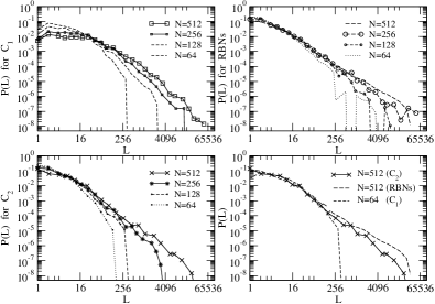
Figure 3: Probability density distribution for the attractor lengths at different fixed network sizes $N$. The four figures correspond respectively to $\mathcal{C}_{1}$ networks, RBNs, canalyzing $\mathcal{C}_{2}$ networks and the comparison of the three classes of networks. In the lower right figure $\mathcal{C}_{1}$ networks with 64 nodes have on average the same number of relevant nodes as $\mathcal{C}_{2}$ networks with 512 nodes. In calculating the relative frequencies of attractor lengths, the frequencies were weighted with the sizes of attractors’ basins of attraction. We considered 1000 initial states for one network realization and averaged over 2000 networks. The data is binned on a logarithmic scale.

We start with probability density for the attractor lengths. The results are presented in Fig. 3. In order to understand them we remind ourselves that the number of relevant nodes $N_{rel}$ scales in $\mathcal{C}_{2}$ networks and RBNs with $N^{1/3}$ , whereas for $\mathcal{C}_{1}$ networks it scales with $\sqrt{N}$. In all cases relevant components of sizes less than $\sim N_{rel}$ are mainly simple loops. The mean number of relevant loops of length $l$ is $1/l$ as long as $l$ is sufficiently far below $N_{rel}$. In the last graph of Fig. 3 (lower right corner) the curves for $N=512$ for RBNs and $\mathcal{C}_{2}$ networks agree well with the curve for $\mathcal{C}_{1}$ networks for $N=64$ for smaller $L$. The reason is that the number of relevant nodes is for all three types of networks of the same size (since $512^{1/3}=64^{1/2}$). The difference for large $L$ is due to the fact that in $\mathcal{C}_{1}$ networks all relevant nodes are on simple loops, so that all relevant components have a cycle period of the order of their size, while the more complex components occuring in the other network types can have much longer cycle lengths. For large $L$, the small difference between $\mathcal{C}_{2}$ networks and RBNs is due to the presence of reversible functions in RBNs: relevant components containing relevant nodes with two relevant inputs and a reversible update function can have extremely long periods, which can become of the order of the state space of the component Kaufman and Drossel (2005).

In our simulations, we find very long attractors also for $\mathcal{C}_{2}$ networks. This fact is fairly surprising if we remember that $\mathcal{C}_{2}$ networks were originally thought to be interesting for their short attractors, see f.i. Kauffman (1969).

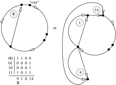
Figure 4: An RBN relevant component and a $\mathcal{C}_{2}$ relevant component, whose attractors can be mapped pairwise onto each other. Triangle arrows represent a chain of nodes, and without loss of generality we can assume that the update functions of the nodes with one input are all a “copy” function. The node marked with its “copy” function is absent in the corresponding right arch of the component on the right, and that arch is thus shorter by one node. The left arch and the straight chain of the left component are identical to the two left arches and the two straight chains of the right component. The table explains the notation for the update functions, 9 being the reversible one, which can be emulated by using the canalyzing functions 1,8, and 14. At the node with the update function $14$ the binary input combination 11 never occurs.

We can explain the appearance of very long attractors in canalyzing networks in the following way. Let us consider a relevant component of an RBN that is a loop with an additional chain of nodes within the loop and a reversible update function at the node with two inputs. As shown in Kaufman and Drossel (2005), the attractors of such a component can comprise a finite proportion of the state space even for very large components. Now, it is possible to construct a relevant component that contains three nodes with two relevant inputs, which all have a canalyzing function, and that has, for the mapping implied by Fig. 4, exactly the same attractor states as the relevant component of the RBN. The number and lengths of attractors is therefore identical in the two components. The reversible function constructed from three canalyzing functions does not, of course, appear as often in $\mathcal{C}_{2}$ networks as a reversible function occurs in the RBN. Therefore the very long attractors appear relatively seldom in canalyzing networks.

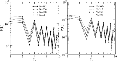
Figure 5: Small-$L$ part of the graphs for $\mathcal{C}_{2}$ networks (left) and RBNs (right) of Fig. 3, without data binning, making visible even-odd oscillations.

In order to produce the curves in Fig. 3 we have binned the data on a logarithmic scale, and we have chosen the binning interval large enough to smoothen quite large fluctuations. Otherwise, we could see even-odd fluctuations in the number of attractors with neighboring lengths, see Fig. 5. There are always more attractors with even lengths. Let us explain this behavior. The small components of the relevant part of $\mathcal{C}_{2}$ networks are simple loops. But for simple loops even attractor lengths appear more often, since a loop with $N_{l}$ nodes leads to attractors of length $N_{l}$ or $2N_{l}$, depending on whether it is even or odd. Therefore, an even attractor length $2N_{l}$ occurs in loops with $2N_{l}$ or $N_{l}$ nodes.

The cutoff in observed attractor length is of the order $L\sim AN^{2}$, with $A=0.1$ for RBN and $0.01$ for $\mathcal{C}_{2}$ networks. This is a finite size effect. Also, full ensemble averages are hard to reproduce numerically. For example, with a substantial probability some network realizations appear with untypically large attractors, which lead to an overestimation of the average attractor length for the considered value of $N$, compare Fig. 6 below.

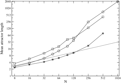
Figure 6: Mean attractor length for canalyzing $\mathcal{C}_{2}$ networks (stars), RBNs (circles) and $\mathcal{C}_{1}$ networks (squares) as a function of network size $N$. The dotted line is a power law $\sqrt{N}$. For the calculation of the mean attractor length, the attractor lengths of different attractors (obtained with 1000 initial states for 2000 networks) were weighted with the corresponding basins of attraction.

Fig. 6 shows our results for the mean length of attractors. The most important observation is that the mean attractor length grows faster than any power law with $N$ for all the considered network classes, including $\mathcal{C}_{2}$ networks, whose attractors are not substantially shorter than those of the other networks. Only for small $N$ can one roughly fit the curves with the $\sqrt{N}$ law suggested a long time ago.

All the curves are similar in shape. The reason for this is again that the relevant part of all three network types consists mainly of simple loops. The mean attractor length of RBNs becomes larger than that of the other two network classes for large $N$, due to the reversible functions occuring in complex components.

We now discuss simulation results for attractor numbers. In analytical calculations Samuelsson and Troein (2003); Drossel (2005), the average number $C_{L}(N_{rel})$ of attractors of length $L$ was found to scale with a power of the number of relevant nodes,

$$C_{L}(N_{rel})\sim N_{rel}^{G_{L}-1}\,,$$ (7)

with a proportionality factor that depends on $L$. $G_{L}$ is closely related to the number of different possible cycles of length $L$ on simple loops. One can approximately write $G_{L}\sim 2^{L}/L$, for details see Drossel (2005), at the end of Section $2$.

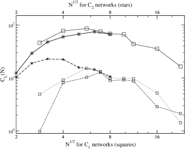
Figure 7: Absolute number of attractors of the lengths $L=7$ (dashed and dotted lines) and $L=8$ (solid lines) for canalyzing $\mathcal{C}_{2}$ networks (stars) and $\mathcal{C}_{1}$ networks (squares). The curves for the different types of networks are plotted in such a way that the abscissae are of the order of the number of relevant nodes for each type. The data were extracted from those used for Fig. 3. The dotted line corresponds to the averaging over 1000 and not 2000 network realizations.

Fig. 7 shows our simulation results for the number of attractors of length $L=7$ and $L=8$ for $\mathcal{C}_{2}$ and $\mathcal{C}_{1}$ networks. The data do not contradict the theoretically predicted scaling with $N_{rel}$ (7), if one realizes the limitations of computer simulations. We considered $1000$ initial states and could therefore explore the state space of a network having typically of the order of not more than 10 relevant nodes. This explains why for $N_{rel}\gtrsim 10$ the number of found attractors decreases with $N_{rel}$ in contrast to the analytical result. On the other hand, the analytical result is only valid for $N_{rel}\gg L$, so that it is simply impossible to see the predicted power law with computer simulations. A remarkable feature of Fig. 7 is the qualitative difference between the curves for even and odd $L$. We know from Drossel (2005) that $G_{L}$ is smaller for odd $L$ than for neighboring even $L$.

Fig. 8 shows the total number of attractors found starting from $1000$ initial states for each network. The curves for the different types of networks are plotted in such a way that the abscissae are of the order of the number of relevant nodes for each type.

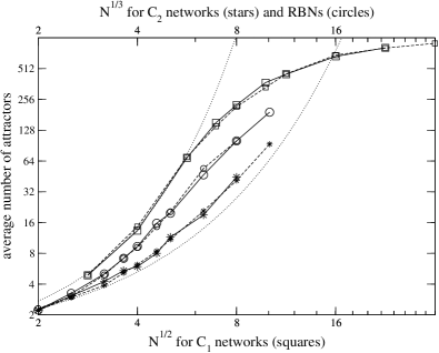
Figure 8: Average number of attractors obtained with $1000$ initial states and $1000$ networks (dashed lines) and $2000$ networks (solid lines) for canalyzing $\mathcal{C}_{2}$ networks (stars), RBNs (circles) and $\mathcal{C}_{1}$ networks (squares). The curves for the different types of networks are plotted in such a way that the abscissae are of the order of the number of relevant nodes for each type. The dotted lines correspond to the curves $2^{0.6\;\mathcal{N}_{1}^{0.5^{\ }}}$ and $2^{0.55\;\mathcal{N}_{1}^{0.7}}$, where $\mathcal{N}_{1}$ is the number of nodes in $\mathcal{C}_{1}$ networks, i.e. the squared value of the abscissa here.

Just as for the previous figure, with $\sim 2^{10}$ random initial states the relevant nodes of a network with $N_{rel}\simeq 10$ assume a large proportion of their possible values, and the average number of attractors found is a good estimate of the real ensemble average (if we average over a sufficiently large number of network samples, compare the dashed and solid line curves in Fig. 8). For much larger networks, it is unlikely that we get the same attractor twice using only $1000$ initial states. Therefore the average number of found attractors trivially approaches $1000$, yielding no information about the network dynamics.

We compared our results with those of Socolar and Kauffman (2003), where numerical simulations were performed to obtain median number of attractors. This number is in our system less than the mean number, and the corresponding curve (not shown) lies below our data. For $\mathcal{C}_{1}$ networks, a lower bound for the average number of attractors is $2^{0.6\sqrt{N}}$, see Drossel et al. (2005). Our data suggest that the number of attractors can well be fitted by $2^{aN^{b}}$ with two constants $a$ and $b$. The lower bound as well as the fit for $\mathcal{C}_{1}$ networks are plotted in Fig. 8 (dotted curves).

Originally based on computer simulation of small systems, Kauffman had suggested that the mean number of attractors increases as $\sqrt{N}$. For small $N$, our data are compatible with such a relation. The newer and analytical results, see f.i. Drossel (2005), lead to the exponentially large number of attractors, also in agreement with our data.

The similarity in the form of the three curves in Fig. 8 confirms our understanding of the dynamics in terms of the relevant nodes. In the limit $N\to\infty$ the fraction of the relevant nodes with two inputs goes to zero for the $\mathcal{C}_{2}$ networks and RBNs and the average number of attractors is mainly determined by of the order of $\ln N$ relevant loops. The average number of attractors grows exponentially fast with the number of relevant nodes.

5 Summary

In this paper, we have shown that canalyzing random Boolean networks have a frozen core, the size of which is comparable to that of other random Boolean networks. It follows that the attractors of canalyzing networks are determined by of the order of $N^{1/3}$ relevant nodes, which are connected to of the order of $\ln N$ relevant components, most of which are simple loops.

We have explained how the frozen core arises starting from self-freezing loops. Furthermore, we have investigated the numbers and lengths of attractors. From the properties of the relevant components it follows that their average numbers increase faster than any power law with system size. Although attractors of canalyzing networks are on average shorter than those of RBNs, extremely long attractors can also arise in canalyzing networks. We have shown this by constructing a relevant component that has the same attractors as a relevant component of an RBN. All the results valid for $\mathcal{C}_{2}$ networks apply also to mixed $\mathcal{C}_{1}$ /$\mathcal{C}_{2}$ networks.

We have also seen that incomplete sampling leads to large fluctuations and uncertainties in the data. Additionally, very short and very long attractors are difficult to find. The first ones constitute an exponentially small fraction of the state space, the others appear exponentially seldom in a network realization. Therefore, computer simulations needed to be supplemented by analytical arguments. At the same time, it is extremely difficult to verify numerically some known analytical results.

We conclude that the original hypothesis that critical canalyzing networks have short attractors cannot be upheld. Rather, biological systems need to be modeled by more specific networks that are not randomly connected.

References

- Kauffman et al. (2003) S. Kauffman, C. Peterson, B. Samuelsson, and C. Troein, Proc. Natl. Acad. Sci. U.S.A. 100, 14796 (2003).
- Kauffman (1969) S. A. Kauffman, J. Theor. Biol. 22, 437 (1969).
- Derrida and Pomeau (1986) B. Derrida and Y. Pomeau, Europhys. Lett. 1, 45 (1986).
- Derrida and Stauffer (1986) B. Derrida and D. Stauffer, Europhys. Lett. 2, 739 (1986).
- Moreira and Amaral (2005) A. A. Moreira and L. A. N. Amaral, Phys. Rev. Lett. 94, 218702 (2005).
- Aldana-Gonzalez et al. (May 2003) M. Aldana-Gonzalez, S. Coppersmith, and L. P. Kadanoff, in Perspectives and Problems in Nonlinear Science, A celebratory volume in honor of Lawrence Sirovich, edited by E. Kaplan, J. E. Mardsen, and K. R. Sreenivasan (Springer Applied Mathematical Sciences Series, Springer Verlag, New York, May 2003), pp. 23–89.
- Bilke and Sjunnesson (2002) S. Bilke and F. Sjunnesson, Phys. Rev. E 65, 016129 (2002).
- Socolar and Kauffman (2003) J. E. S. Socolar and S. A. Kauffman, Phys. Rev. Lett. 90, 068702 (2003).
- Samuelsson and Troein (2003) B. Samuelsson and C. Troein, Phys. Rev. Lett. 90, 098701 (2003).
- Gershenson (2004) C. Gershenson, in Artificial Life IX, Proceedings of the Ninth International Conference on the Simulation and Synthesis of Living Systems, edited by J. Pollack, M. Bedau, P. Husbands, T. Ikegami, and R. A. Watson (MIT Press, 2004), pp. 238–243.
- Klemm and Bornholdt (2005) K. Klemm and S. Bornholdt (2005), accepted for publication in Phys. Rev. E, eprint cond-mat/0411102.
- Drossel (2005) B. Drossel, Phys. Rev. E 72, 016110 (2005).
- Kaufman et al. (2005) V. Kaufman, T. Mihaljev, and B. Drossel, Phys. Rev. E 72, 046124 (2005).
- Drossel et al. (2005) B. Drossel, T. Mihaljev, and F. Greil, Phys. Rev. Lett. 94, 088701 (2005).
- Kaufman and Drossel (2005) V. Kaufman and B. Drossel, Eur. Phys. J. B 43, 115 (2005).