Lattice thermal conductivity of disordered binary alloys I : a formulation

Abstract

We present here a formulation for the calculation of the configuration averaged lattice thermal conductivity in random alloys. Our formulation is based on the augmented-space theorem, introduced by one of us am , combined with a generalized diagrammatic technique. The diagrammatic approach simplifies the problem of including effects of disorder corrections to a great extent. The approach allows us to obtain an expression for the effective heat current in case of disordered alloys, which in turn is used in a Kubo-Greenwood type formula for the thermal conductivity. We show that disorder scattering renormalizes the phonon propagators as well as the heat currents. The corrections to the current terms have been shown to be related to the self-energy of the propagators. We also study the effect of vertex corrections in a simplified ladder diagram approximation. A mode dependent diffusivity $D_{\gamma}$ and then a total thermal diffusivity averaged over different modes are defined. Schemes for implementing the said formalism are discussed. A few initial numerical results on the frequency and temperature dependence of lattice thermal conductivity are presented for NiPd alloy and are also compared with experiment. We also display numerical results on the frequency dependence of thermal diffusivity averaged over modes.

I Introduction

The problem of phonon excitations have been studied extensively both theoretically and experimentally in mixed crystals elliot ; kambrock as well as in insulators maradudin . However, there are far fewer studies of lattice thermal conductivity in disordered alloys. Detailed comparison between theory and experiment on the basis of realistic models has not been extensive. Model calculations are mostly based on mass disorder, whereas in phonon problems essential off-diagonal disorder in the force constants cannot be dealt within single site mean-field approximations. Such disorder cannot be ignored in a realistic calculation.

In the past few decades, there has been considerable attention directed towards the theoretical understanding of the lattice thermal conductivity of metals. These are mainly due to the efforts of Klemens klemens , Ziman ziman , Callaway call , Parrot parrot and others. However majority of these were based on model calculations, either for perfect crystals or ordered alloys. Flicker and Leath FL first proposed the calculation of lattice thermal conductivity within a single-site coherent potential approximation (CPA) using the appropriate Kubo formula. The single-site CPA is a mean field approximation, capable of dealing with mass disorder alone and is not adequate for treating intrinsic off-diagonal disorder arising out of the force constants. This was evidenced in the inability of the single site CPA to explain experimental life time data on NiPt Tsunoda . Translationally invariant, multiple site, multiple scattering theories based on the augmented space formalism am have recently been proposed by Ghosh et.al. glc as well as by us am1 to describe phonons in a series of random alloy systems : NiPt, NiPd and NiCr. These formalisms explicitly capture the effects of both the diagonal and off-diagonal disorder.

In this paper, we shall first introduce a Kubo-Greenwood type formula which relates the thermal conductivity to the (heat) current-current correlation function. The ideas used here are very similar to those proposed by Allen and Feldman af except that the present formulation is done keeping in mind the application to a substitutionally disordered crystal, rather than an amorphous system. For disordered alloys, configuration averaging over various random atomic arrangements have been carried out using the augmented space formalism (ASF) introduced by us am . The ASF goes beyond the usual mean-field approaches and takes into account configuration fluctuations over a large local environment. We shall combine the augmented space representation for phonons am1 with a scattering diagrammatic technique to get an effective heat current. This effective current consists in addition to the averaged current term, also the terms arising out of the disorder scattering corrections. We will show that these disorder induced corrections to the averaged current terms are directly related either to the disorder scattering induced self-energy matrix in the propagator or to vertex corrections. As far as the vertex corrections are concerned, Leath leath had obtained these corrections within the framework of CPA by using diagram summations. In this paper we shall derive the contribution of these corrections in a more generalized context with the inclusion of diagonal as well as the intrinsic off-diagonal disorder arising out of the dynamical matrix. Since in an earlier communication am2 we have already shown that the self energy matrix and the Green matrix can be calculated for realistic binary alloys within an augmented space block recursion (ASBR) technique, so the present formulation will form the basis of a subsequent calculation of lattice thermal conductivity in realistic alloys.

The rest of the paper is organized as follows. In Sec. II, we describe the basic tools used to calculate the lattice thermal conductivity for a crystal. In Sec. III(A), we briefly introduce the augmented space representation for phonons. In Sec. III(B,C), we derive expressions for important physical quantities such as effective heat current, averaged lattice thermal conductivity and thermal diffusivity in terms of configuration averaged Green matrix and self energy matrix of the system. In Sec. III(D), we describe vertex corrections arising out of the correlated propagation. Sec. IV(A,B) is devoted for a description of the schemes for implementing this formalism to realistic alloys. Few of the initial numerical results on the lattice thermal conductivity and thermal diffusivity for NiPd alloy are shown in Sec. V and an effort has been put forward to compare them with the available experimental data. Concluding remarks appear in Sec. VI.

II Thermal conductivity

In an earlier work sm we had reported a formulation for the study of optical conductivity in disordered alloys. Here we attempt to modify that formulation for lattice thermal conductivity studies also in disordered alloys. The formulations have similar overall similarities, but differ in specific details, which we would like to focus on in this communication. The Kubo formula which relates the optical conductivity to a current-current correlation function is well established. The Hamiltonian contains a term $\sum_{i}{\mathbf{j}}_{i}\cdot{\mathbf{A}}({{\mathbf{r}}_{i}},t)$ which drives the electrical current. For thermal conductivity we do not have a similar term in the Hamiltonian which drives a heat current. The derivation of a Kubo formula in this situation requires an additional statistical hypothesis af , which states that a system in steady state has a space dependent local temperature $T({{\mathbf{r}}_{i}})=[\kappa_{B}\beta({{\mathbf{r}}_{i}})]^{-1}$. The expression for the heat current has been discussed in great detail by Hardy hardy and Allen and Feldman af . The readers are refereed to these papers for the details of calculation. The matrix element of the heat current in the basis of the eigenfunctions of the Hamiltonian is given by :

$${\mathbf{S}}_{\gamma\gamma^{\prime}}^{\mu}({\mathbf{k}}\ )\ =\ \frac{\hbar}{2}\ \left(\rule{0.0pt}{8.53581pt}\omega_{{\mathbf{k}}\ \gamma}+\omega_{{\mathbf{k}}\ \gamma^{\prime}}\right)\ {\mathbf{v}}^{\mu}_{\gamma\gamma^{\prime}}({\mathbf{k}}\ ),$$ (1)

where, the phonon group velocity ${\mathbf{v}}_{\gamma\gamma^{\prime}}({\mathbf{k}}\ )$ is given by

$${\mathbf{v}}_{\gamma\gamma^{\prime}} = \frac{i}{2\sqrt{\omega_{{\mathbf{k}}\ \gamma}\omega_{{\mathbf{k}}\ \gamma^{\prime}}}}\ \sum_{\mu}\sum_{\nu}\epsilon^{\mu}_{\gamma}({\mathbf{k}}\ )\ \epsilon^{\nu}_{\gamma^{\prime}}({\mathbf{k}}\ )$$

$$\left(\sum_{\mathbf{R}_{ij}}\ \frac{\Phi^{\mu\nu}({\mathbf{R}_{ij}})}{\sqrt{M_{i}M_{j}}}\ \right){\mathbf{R}}_{ij}\ e^{i{\mathbf{k}}\ \cdot{\mathbf{R}}_{ij}}$$

$$= \frac{1}{2\sqrt{\omega_{{\mathbf{k}}\ \gamma}\omega_{{\mathbf{k}}\ \gamma^{\prime}}}}\ \sum_{\mu}\sum_{\nu}\epsilon^{\mu}_{\gamma}({\mathbf{k}}\ )\ {\mathbf{\nabla}}_{\mathbf{k}}\ D^{\mu\nu}({\mathbf{k}}\ )\ \epsilon^{\nu}_{\gamma^{\prime}}({\mathbf{k}}\ ),$$

here $\gamma,\gamma^{\prime}$ label the various modes of vibration, $\omega_{{\mathbf{k}}\ \gamma},\omega_{{\mathbf{k}}\ \gamma^{\prime}}$ are their frequencies, $\epsilon^{\mu}_{\gamma}({\mathbf{k}}\ ),\epsilon^{\nu}_{\gamma^{\prime}}({\mathbf{k}}\ )$ are the polarization vectors and $D^{\mu\nu}({\mathbf{k}}\ )$ is the Fourier transform of mass scaled dynamical matrix.

We shall consider the case where the temperature gradient is uniform within the system. The Kubo formula then relates the linear heat current response to the temperature gradient field

$$\langle S^{\mu}(t)\rangle=-\sum_{\nu}\int_{-\infty}^{\infty}\ dt^{\prime}\ \kappa^{\mu\nu}(t-t^{\prime})\ {\mathbf{\nabla}}^{\nu}\delta T(t),$$

where

$$\kappa^{\mu\nu}(\tau)=\Theta(\tau)\ \frac{1}{T}\int_{0}^{\beta}\ d\lambda\langle S^{\mu}(-i\hbar\lambda),S^{\nu}(\tau)\rangle,$$

$\Theta(\tau)$ is the Heaviside step function, and

$$S(-i\hbar\lambda)\ =\ e^{\lambda H}\ S\ e^{-\lambda H}.$$

$\langle\ \rangle$ on the right-hand side of the above equation denotes thermal averaging over states in the absence of the temperature gradient. The above equation can be rewritten in the form of a Kubo-Greenwood expression

$$\kappa^{\mu\nu}(\omega,T) = \ \kappa^{\mu\nu}_{I}(\omega,T)\ +\ \kappa^{\mu\nu}_{II}(\omega,T)$$

$$\kappa^{\mu\nu}_{I}(\omega,T) = \frac{\pi}{T}\ \int\frac{d^{3}{\mathbf{k}}\ }{8\pi^{3}}\ \sum_{\gamma}\sum_{\gamma^{\prime}\neq\gamma}\ \frac{\langle n_{{\mathbf{k}}\ \gamma^{\prime}}\rangle-\langle n_{{\mathbf{k}}\ \gamma}\rangle}{\hbar(\omega_{{\mathbf{k}}\ \gamma}-\omega_{{\mathbf{k}}\ \gamma^{\prime}})}$$

$${\mathbf{S}}^{\mu}_{\gamma\gamma^{\prime}}({\mathbf{k}}\ ){\mathbf{S}}^{\nu}_{\gamma^{\prime}\gamma}({\mathbf{k}}\ )\ \delta(\omega_{{\mathbf{k}}\ \gamma}-\omega_{{\mathbf{k}}\ \gamma^{\prime}}-\omega)$$

(3)

$$\kappa^{\mu\nu}_{II}(\omega,T) = \frac{1}{\kappa_{B}T^{2}}\left[\rule{0.0pt}{11.38109pt}\left\{\int\frac{d^{3}{\mathbf{k}}\ }{8\pi^{3}}\sum_{\gamma}\langle n_{{\mathbf{k}}\ \gamma}\rangle\ {\mathbf{S}}^{\mu}_{\gamma\gamma}({\mathbf{k}}\ )\right\}\right.$$ (4)

$$\left.\left\{\int\frac{d^{3}{\mathbf{k}}\ }{8\pi^{3}}\sum_{\gamma}\langle n_{{\mathbf{k}}\ \gamma}\rangle\ {\mathbf{S}}^{\nu}_{\gamma\gamma}({\mathbf{k}}\ )\right\}-\kappa_{B}T\int\frac{d^{3}{\mathbf{k}}\ }{8\pi^{3}}\right.$$

$$\left.\sum_{\gamma}\frac{\partial\langle n_{{\mathbf{k}}\ \gamma}\rangle}{\partial(\hbar\omega_{{\mathbf{k}}\ \gamma})}\ S^{\mu}_{\gamma\gamma}({\mathbf{k}}\ )\ S^{\nu}_{\gamma\gamma}({\mathbf{k}}\ )\right]\delta(\omega),$$

where $\langle n_{{\mathbf{k}}\ \gamma}\rangle=(e^{\beta\hbar\omega_{{\mathbf{k}}\ \gamma}}-1)^{-1}$ is the equilibrium Bose Einstein distribution function and T is the absolute temperature.

The first expression is for inter-band transitions, while the second expression is for intra-band transitions. For an isotropic response, we can rewrite the first expression as

$$\kappa_{I}(\omega,T) = \frac{\pi}{3T}\sum_{\mu}\int\ d\omega^{\prime}\int\frac{d^{3}{\mathbf{k}}\ }{8\pi^{3}}\sum_{\gamma}\sum_{\gamma^{\prime}}\widehat{\mathbf{S}}^{\mu}_{\gamma\gamma^{\prime}}({\mathbf{k}}\ ,T)$$

$$\widehat{\mathbf{S}}^{\mu}_{\gamma^{\prime}\gamma}({\mathbf{k}}\ ,T)\delta(\omega^{\prime}-\omega_{{\mathbf{k}}\ \gamma^{\prime}})\delta(\omega^{\prime}+\omega-\omega_{{\mathbf{k}}\ \gamma}),$$

where

$$\widehat{\mathbf{S}}^{\mu}_{\gamma\gamma^{\prime}}({\mathbf{k}}\ ,T)\ =\ \sqrt{\left|\frac{\langle n_{{\mathbf{k}}\ \gamma^{\prime}}\rangle-\langle n_{{\mathbf{k}}\ \gamma}\rangle}{\hbar(\omega_{{\mathbf{k}}\ \gamma}-\omega_{{\mathbf{k}}\ \gamma^{\prime}})}\right|}\ {\mathbf{S}}^{\mu}_{\gamma\gamma^{\prime}}({\mathbf{k}}\ ).$$

We may rewrite the above equation as

$$\kappa_{I}(\omega,T) = \frac{1}{3\pi T}\ \sum_{\mu}\ \int d\omega^{\prime}\int\frac{d^{3}{\mathbf{k}}\ }{8\pi^{3}}\mbox{Tr}\left[\rule{0.0pt}{11.38109pt}\ \widehat{\mathbf{S}}^{\mu}({\mathbf{k}}\ ,T)\right.$$

$$\left.\Im m\{{\mathbf{G}}({\mathbf{k}}\ ,\omega^{\prime})\}\ \widehat{\mathbf{S}}^{\mu}({\mathbf{k}}\ ,T)\ \Im m\{{\mathbf{G}}({\mathbf{k}}\ ,\omega^{\prime}+\omega)\}\right].$$

The operator G($\omega$) is the phonon Green operator $(M\omega^{2}{\mathbf{I}}-{\mathbf{\Phi}})^{-1}$. The Trace is invariant in different representations. For crystalline systems, usually the Bloch basis $\{|{\mathbf{k}},\gamma\rangle\}$ is used. For disordered systems, prior to configuration averaging, it is more convenient to use the basis $\{|{\mathbf{k}}\ ,\alpha\rangle\}$, where ${\mathbf{k}}\$ is the reciprocal vector and $\alpha$ represents the coordinate axes directions. We can transform from the mode basis to the coordinate basis by using the transformation matrices $\Upsilon_{\gamma\alpha}({\mathbf{k}}\ )=\ \epsilon^{\alpha}_{\gamma}({\mathbf{k}}\ )$. For example

$$\widehat{\mathbf{S}}_{\alpha\beta}^{\mu}({\mathbf{k}}\ ,T)\ =\ \Upsilon^{-T}_{\alpha\gamma}({\mathbf{k}}\ )\ \widehat{\mathbf{S}}^{\mu}_{\gamma\gamma^{\prime}}({\mathbf{k}}\ ,T)\ \Upsilon^{-1}_{\gamma^{\prime}\beta}({\mathbf{k}}\ ).$$

If we define

$${\mathbf{\kappa}}(z_{1},z_{2})=\int\frac{d^{3}{\mathbf{k}}\ }{8\pi^{3}}\ \mbox{Tr}\left[\ \rule{0.0pt}{11.38109pt}\widehat{\mathbf{S}}\ {\mathbf{G}}({\mathbf{k}}\ ,z_{1})\ \widehat{\mathbf{S}}\ {\mathbf{G}}({\mathbf{k}}\ ,z_{2})\right].$$ (5)

then the above equation becomes,

$$\kappa_{I}(\omega,T) = \frac{1}{12\pi T}\ \sum_{\mu}\int d\omega^{\prime}\ \left[\rule{0.0pt}{11.38109pt}{\mathbf{\kappa}}^{\mu\mu}(\omega^{\prime-},\omega^{\prime+}+\omega)\right.$$ (6)

$$\left.+{\mathbf{\kappa}}^{\mu\mu}(\omega^{\prime+},\omega^{\prime-}+\omega)-{\mathbf{\kappa}}^{\mu\mu}(\omega^{\prime+},\omega^{\prime+}+\omega)\right.$$

$$\left.-{\mathbf{\kappa}}^{\mu\mu}(\omega^{\prime-},\omega^{\prime-}+\omega)\right]\rule{0.0pt}{11.38109pt},$$

where

$$f(\omega^{+})=\lim_{\delta\rightarrow 0}f(\omega+i\delta),\phantom{xx}f(\omega^{-})=\lim_{\delta\rightarrow 0}f(\omega-i\delta).$$

We have used the herglotz analytic property am1 of the Green operator

$${\mathbf{G}}(\omega+i\delta)=\Re e\left[\rule{0.0pt}{8.53581pt}{\mathbf{G}}(\omega)\right]\enskip-\enskip i\ \mbox{sgn}(\delta)\ \Im m\left[\rule{0.0pt}{8.53581pt}{\mathbf{G}}(\omega)\right].$$

For disordered materials, we shall be interested in obtaining the configuration averaged response functions. This will require the configuration averaging of quantities like $\kappa(z_{1},z_{2})$

We should note that the expressions (5) and (6) are similar to the corresponding equations for optical conductivity, with the heat current replacing electrical current. To deal with random alloys we shall follow an analogous procedure for optical conductivity proposed earlier sm

III Configuration averaging

III.1 The augmented space formalism for phonons

The augmented space formalism (ASF) has been described in detail in several earlier papers (see mook2 -mook3 ). We shall, for the sake of completeness, describe only those features which will be necessary for the implementation of our ideas in this communication. It is also important to introduce the notations used subsequently. The theory of phonons consists of solving a secular equation of the form

$$({\bf M}w^{2}-{\bf D})\ {\bf u}(R,w)=0,$$

where $u_{\alpha}(R,w)$ is the Fourier transform of $u_{\alpha}(R,t)$, the displacement of an atom from its equilibrium position $R$ on the lattice, in the direction ${\alpha}$ at time $t$. M is the mass operator, diagonal in real-space and D is the dynamical matrix operator whose tight-binding representations are

$${\bf M} = \sum_{R}m_{R}\ {\delta}_{\alpha\beta}\ P_{R},$$

$${\bf D} = \sum_{R}\left\{\sum_{R^{\prime}\neq R}\Phi_{RR^{\prime}}^{\alpha\beta}\right\}\ P_{R}+\sum_{R}\sum_{R^{\prime}\neq R}\Phi_{RR^{\prime}}^{\alpha\beta}\ T_{RR^{\prime}},$$

where the sum rule has been incorporated in the first term of the equation involving $\bf D$.
Here $P_{R}$ is the projection operator $|R\rangle\langle R|$  and $T_{RR^{\prime}}$ is the transfer operator $|R\rangle\langle R^{\prime}|$  in the Hilbert space ${\cal H}$ spanned by the tight-binding basis $\{|R\rangle\}$. $R,R^{\prime}$ specify the lattice sites and $\alpha$,$\beta$ the Cartesian directions. $m_{R}$ is the mass of an atom occupying the position $R$ and $\Phi_{RR^{\prime}}^{\alpha\beta}$ is the force constant tensor.

We shall be interested in calculating the displacement-displacement Green matrix ${\mathbf{G}}(R,R^{\prime},w^{2})$

$${\mathbf{G}}(R,R^{\prime},w^{2})=\langle R|\left({\bf{M}}w^{2}-{\bf{D}}\right)^{-1}|R^{\prime}\rangle.$$

Let us now consider a binary alloy $A_{x}B_{y}$ consisting of two kinds of atoms A and B of masses $m_{A}$ and $m_{B}$ randomly occupying each lattice sites. We wish to calculate the configuration-averaged Green matrix $\ll{\bf G}({R,R^{\prime}},w^{2})\gg$. We shall use the augmented space formalism to do so indicating the main operational results here. For further details we refer the reader to the monograph tf . The first operation is to represent the random parts of the secular equation in terms of a random set of local variables $\{n_{R}\}$ which are 1 if the site $R$ is occupied by an A atom and 0 if it is occupied by B. The probability densities of these variables may be written as

$$Pr(n_{R}) = x\ \delta(n_{R}-1)\ +\ y\ \delta(n_{R})$$ (8)

$$= (-1/{\pi})\ \Im m\langle{\uparrow}_{R}|\ (n_{R}I-{\it{N_{R}}})^{-1}\ |{\uparrow}_{R}\rangle,$$

where $x$ and $y$ are the concentrations of the constituents A and B with $x+y=1$. $N_{R}$ is an operator defined on the configuration-space $\phi_{R}$ of the variable $n_{R}$. This is of rank $2$ and is spanned by the states $\{|{\uparrow_{R}}\rangle,|{\downarrow_{R}}\rangle\}$,

$$|\uparrow_{R}\rangle\ =\ \sqrt{x}|A_{R}\rangle+\sqrt{y}|B_{R}\rangle,\quad|\downarrow_{R}\rangle\ =\ \sqrt{y}|A_{R}\rangle-\sqrt{x}|B_{R}\rangle,$$

$$N_{R}=xp_{R}^{\uparrow}+yp_{R}^{\downarrow}+\sqrt{xy}\ {\cal T}^{\uparrow\downarrow}_{R},\quad\quad{\cal T}^{\uparrow\downarrow}_{R}\ =\ {\tau}^{\uparrow\downarrow}_{R}+{\tau}^{\downarrow\uparrow}_{R},$$

where $|A_{R}\rangle$ is the state in which an atom of the type A occupies a site $R$. $|B_{R}\rangle$ is similarly defined. $p_{R}^{\uparrow}=|\uparrow_{R}\rangle\langle\uparrow_{R}|$ and $p_{R}^{\downarrow}=|\downarrow_{R}\rangle\langle\downarrow_{R}|$ are projection operators and ${\tau}_{R}^{\uparrow\downarrow}=|\uparrow_{R}\rangle\langle\downarrow_{R}|$ and ${\tau}_{R}^{\downarrow\uparrow}=|\downarrow_{R}\rangle\langle\uparrow_{R}|$ are transfer operators in the configuration space $\phi_{R}$.

In terms of random variables $n_{R}$, the mass operator can be written as

$${\bf M}\ =\ \sum_{R}\left[\rule{0.0pt}{11.38109pt}m_{B}\ +\ n_{R}\ (\delta m)\right]\delta_{\alpha\beta}\ P_{R},\quad\quad\delta m=m_{A}-m_{B}$$ (9)

According to the augmented space theorem, in order to obtain the configuration-average we simply replace the random variables $n_{R}$ by the corresponding operators $N_{R}$ associated with its probability density, as in Eqn. (8), and take the matrix element of the resulting operator between the reference states. For a full mathematical proof the reader is referred to tf .

$$n_{R}\longrightarrow N_{R}\ =\ x\ \tilde{I}\ +\ (y-x)\ p_{R}^{\downarrow}+\sqrt{xy}\ {\cal T}^{\uparrow\downarrow}_{R}.$$

Using the above we get,

$$\widetilde{\bf M} = {\mathbf{A}}({\mathbf{m}})\ \widetilde{I}\otimes I+{\mathbf{B}}({\mathbf{m}})\ \sum_{R}p_{R}^{\downarrow}\otimes P_{R}$$

$$+{\mathbf{F}}({\mathbf{m}})\ \sum_{R}\ {\cal T}^{\uparrow\downarrow}_{R}\otimes P_{R}$$

$$= \ll\widetilde{\mathbf{M}}\gg\ +\ \widetilde{\mathbf{M}}^{\prime},$$ (10)

where

$$\begin{array}[]{ll}{\mathbf{A}}({\mathbf{X}})=\ll{\mathbf{X}}\gg\ =(x{\mathbf{X}}_{A}+y{\mathbf{X}}_{B}),\\ {\mathbf{B}}({\mathbf{X}})=(y-x)\ ({\mathbf{X}}_{A}-{\mathbf{X}}_{B}),\\ {\mathbf{F}}({\mathbf{X}})=\sqrt{xy}\ ({\mathbf{X}}_{A}-{\mathbf{X}}_{B}).\end{array}$$

Similarly the random off-diagonal force constants $\Phi_{RR^{\prime}}^{\alpha\beta}$ between the sites $R$ and $R^{\prime}$ can be written as

$$\Phi_{RR^{\prime}}^{\alpha\beta} = \Phi_{AA}^{\alpha\beta}n_{R}n_{R^{\prime}}+\Phi_{BB}^{\alpha\beta}(1-n_{R})(1-n_{R^{\prime}})+$$

$$\Phi_{AB}^{\alpha\beta}\left[\rule{0.0pt}{11.38109pt}\ n_{R}(1-n_{R^{\prime}})+n_{R^{\prime}}(1-n_{R})\ \right]$$

$$= \Phi_{BB}^{\alpha\beta}\ +\ \left(\rule{0.0pt}{11.38109pt}\Phi_{AA}^{\alpha\beta}+\Phi_{BB}^{\alpha\beta}-2\Phi_{AB}^{\alpha\beta}\right)\ n_{R}n_{R^{\prime}}+$$

$$\left(\rule{0.0pt}{11.38109pt}\Phi_{AB}^{\alpha\beta}-\Phi_{BB}^{\alpha\beta}\right)\ (n_{R}+n_{R^{\prime}}).$$

Let us define the following :

$$\Phi^{\alpha\beta}_{(1)} = x\ \Phi_{AA}^{\alpha\beta}-y\ \Phi_{BB}^{\alpha\beta}+(y-x)\Phi_{AB}^{\alpha\beta},$$

$$\Phi^{\alpha\beta}_{(2)} = \Phi_{AA}^{\alpha\beta}+\Phi_{BB}^{\alpha\beta}-2\Phi_{AB}^{\alpha\beta}.$$

In augmented space the off-diagonal force constant matrix becomes an operator

$$\widetilde{\mathbf{D}}^{\alpha\beta}_{(off)} = \sum_{RR^{\prime}}\ \left[\rule{0.0pt}{14.22636pt}\ll\Phi^{\alpha\beta}_{RR^{\prime}}\gg\ \tilde{I}+\Phi^{\alpha\beta}_{(1)}\left\{(y-x)\ (p^{\downarrow}_{R}+p^{\downarrow}_{R^{\prime}})\right.\right.$$

$$\left.\left.+\sqrt{xy}({\cal T}^{\uparrow\downarrow}_{R}+{\cal T}^{\uparrow\downarrow}_{R^{\prime}})\right\}+\Phi^{\alpha\beta}_{(2)}\ \left\{(y-x)^{2}\ p^{\downarrow}_{R}\ p^{\downarrow}_{R^{\prime}}+\right.\right.$$

$$\left.\left.\sqrt{xy}(y-x)\left(p^{\downarrow}_{R}{\cal T}^{\uparrow\downarrow}_{R^{\prime}}+p^{\downarrow}_{R^{\prime}}{\cal T}^{\uparrow\downarrow}_{R}\right)+xy{\cal T}^{\uparrow\downarrow}_{R}{\cal T}^{\uparrow\downarrow}_{R^{\prime}}\right\}\rule{0.0pt}{14.22636pt}\right]\otimes T_{RR^{\prime}}$$

$$= \sum_{RR^{\prime}}\ll\Phi^{\alpha\beta}_{RR^{\prime}}\gg\tilde{I}\otimes T_{RR^{\prime}}+\sum_{RR^{\prime}}\ \Psi_{RR^{\prime}}^{\alpha\beta}\otimes T_{RR^{\prime}}.$$

The sum rule gives the diagonal element,

$$\widetilde{\mathbf{D}}^{\alpha\beta}_{(dia)} = -\sum_{R}\left\{\rule{0.0pt}{2.84526pt}\sum_{R^{\prime}\neq R}\ll\Phi^{\alpha\beta}_{RR^{\prime}}\gg\widetilde{I}\right\}\otimes P_{R}$$

$$-\sum_{R}\ \left\{\sum_{R^{\prime}\neq R}\Psi_{RR^{\prime}}^{\alpha\beta}\right\}\otimes P_{R}$$

The total dynamical matrix in the augmented space is

$$\widetilde{\mathbf{D}} \ =\ \ll\widetilde{\mathbf{D}}\gg-\sum_{R}\ \left\{\sum_{R^{\prime}\neq R}\Psi_{RR^{\prime}}^{\alpha\beta}\right\}\otimes P_{R}\$$

$$\ +\ \sum_{RR^{\prime}}\ \Psi_{RR^{\prime}}^{\alpha\beta}\otimes T_{RR^{\prime}}$$

$$\ =\ \ll\widetilde{\mathbf{D}}\gg\ +\ \widetilde{\mathbf{D}}^{\prime}.$$ (12)

The boldface operators are $3\times 3$ matrix representations in the three Cartesian directions.

The augmented space theorem am now states that the configuration-average of the Green matrix $\ll~{}{\bf G}({R,R^{\prime}},w^{2})~{}\gg$ may be written as

$$\ll{\mathbf{G}}\left({R,R^{\prime}},w^{2}\right)\gg\phantom{xxxxxxxxxxxxxxxxxxxxxx}$$

$$\phantom{xxx}=\langle\{\emptyset\}\otimes R|\ \left(\widetilde{\bf{M}}\ w^{2}-\widetilde{\bf{D}}\right)^{-1}\ |\{\emptyset\}\otimes R^{\prime}\rangle\ ,\phantom{xx}$$ (13)

where $\widetilde{\bf{M}}$ and $\widetilde{\bf{D}}$ are the operators which are constructed out of ${\bf{M}}$ and ${\bf{D}}$ by replacing all the random variables $n_{R}$ (or $n_{R^{\prime}})$ by the corresponding operators $N_{R}$ (or $N_{R^{\prime}})$ as given by Eqn.(10) and (12). These are the operators in the augmented space $\Omega={\cal H}\otimes\Phi$. The state $|{R}\otimes\{\emptyset\}\rangle$ is a state in the augmented space, which is the direct product of the real-space and the configuration-space bases.The configuration-space $\Phi=\prod_{R}^{\otimes}\phi_{R}$ is of rank $2^{N}$ for a system of N-lattice sites with binary distribution. A basis in this space is denoted by the cardinality sequence $\{{\cal C}\}=\{R_{1},R_{2},\ldots,R_{c}\}$ which gives us the positions where we have a $|\!\downarrow\rangle$ configuration. The configuration $\{\emptyset\}$ refers to a null cardinality sequence i.e. one in which we have $|\uparrow\rangle$ at all sites.

The virtual crystal (VCA) Green matrix is

$${\mathbf{g}}({R,R^{\prime}},w^{2})=\langle\{\emptyset\}\otimes R|(\ll\widetilde{\mathbf{M}}\gg\omega^{2}-\ll\widetilde{\bf D}\gg)^{-1}|\{\emptyset\}\otimes R^{\prime}\rangle,$$ (14)

where

$$\ll\widetilde{\mathbf{M}}\gg=\ll m\gg\widetilde{I}\otimes I.$$

Referring back to Equations (10),(12) and (13) we get

$$\ll{\mathbf{G}}(R,R^{\prime},w^{2})\gg = \langle\{\emptyset\}\otimes R|\ \left(\rule{0.0pt}{11.38109pt}\ll\widetilde{\mathbf{M}}\gg\omega^{2}-\ll\widetilde{\bf D}\gg\right.$$

$$\left.+\ \widetilde{\mathbf{M}}^{\prime}\omega^{2}-\widetilde{\mathbf{D}}^{\prime}\right)^{-1}\ |\{\emptyset\}\otimes R^{\prime}\rangle$$

$$= \langle\{\emptyset\}\otimes R|\left({\mathbf{g}}^{-1}-\widetilde{\mathbf{D}}_{1}\right)^{-1}|\{\emptyset\}\otimes R^{\prime}\rangle,$$

(15)

we define

$$\widetilde{\mathbf{D}}_{1} = \sum_{R}\ \left\{\rule{0.0pt}{14.22636pt}{-\mathbf{\Upsilon}}_{R}-\sum_{R^{\prime}\neq R}{\mathbf{\Psi}}_{RR^{\prime}}\right\}\ \otimes P_{R}+$$

$$\sum_{R}\sum_{R^{\prime}\neq R}\ {\mathbf{\Psi}}_{RR^{\prime}}\otimes T_{RR^{\prime}}$$

with

$${\mathbf{\Upsilon}}_{R} = {\mathbf{B}}({\mathbf{m}})\ w^{2}\ p^{\downarrow}_{R}\ +\ {\mathbf{F}}({\mathbf{m}})\ w^{2}\ {\cal T}^{\uparrow\downarrow}_{R}$$

$${\mathbf{\Psi}}_{RR^{\prime}} = {\mathbf{D}}^{(1)}_{RR^{\prime}}\ \left(p^{\downarrow}_{R}+p^{\downarrow}_{R^{\prime}}\right)+{\mathbf{D}}^{(2)}_{RR^{\prime}}\ \left({\cal T}^{\uparrow\downarrow}_{R}+{\cal T}^{\uparrow\downarrow}_{R^{\prime}}\right)+$$ (16)

$${\mathbf{D}}^{(3)}_{RR^{\prime}}\ p^{\downarrow}_{R}\ p^{\downarrow}_{R^{\prime}}+{\mathbf{D}}^{(4)}_{RR^{\prime}}\ \left(p^{\downarrow}_{R}\ {\cal T}^{\uparrow\downarrow}_{R^{\prime}}+{\cal T}^{\uparrow\downarrow}_{R}\ p^{\downarrow}_{R^{\prime}}\right)$$

$$+\ {\mathbf{D}}^{(5)}_{RR^{\prime}}\ {\cal T}^{\uparrow\downarrow}_{R}\ {\cal T}^{\uparrow\downarrow}_{R^{\prime}},$$

where

$${\mathbf{D}}^{(1)} = (y-x)\ \Phi_{(1)},$$

$${\mathbf{D}}^{(2)} = \sqrt{xy}\ \Phi_{(1)},$$

$${\mathbf{D}}^{(3)} = {(y-x)^{2}}\ \Phi_{(2)},$$

$${\mathbf{D}}^{(4)} = \sqrt{xy}\ (y-x)\ \Phi_{(2)},$$

$${\mathbf{D}}^{(5)} = xy\ \Phi_{(2)}.$$

Scattering diagrams are obtained by expanding the Eq. (15) as an infinite series and the terms B, F and D⁽¹⁾ to D⁽⁵⁾ are represented as scattering vertices (see Fig. 1).

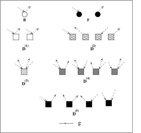
Figure 1: The scattering vertices for the averaged Green function

It might be instructive to understand what these scattering vertices represent physically. If we look at Eq. (15), we note that the term $\widetilde{\mathbf{D}}_{1}$ leads to the creation or annihilation of configuration fluctuations over and above the virtual crystal description. The vertices F shown in Fig 1, create and annihilate a configuration fluctuation at a given site because of mass disorder, while the vertex B counts the number of such fluctuations at a given site. These are the only type of configuration fluctuations we can have if we had single site mass disorder alone. The single-site mean-field approximations like the single-site coherent potential approximation (1CPA) can ideally deal with situations where we ignore the other vertices in Fig 1.

The vertices D⁽²⁾ also describe creation and annihilation of configuration fluctuations at single sites. That is, fluctuations at any one end of the two-site dynamical matrix. Similarly, the vertices D⁽¹⁾ count the number of configuration fluctuations at any one of the two ends of the dynamical matrix. These are also single-site configuration fluctuations but arise due to fluctuations in the two-site dynamical matrix. These may also be treated with some variant of the 1CPA. For example, there are versions of the 1CPA which assume 2D^AB = D^AA + D^BB. With such an assumption only the single site configurations fluctuation vertices are non-zero.

The vertices D⁽⁵⁾ describe creation and annihilation of two configuration fluctuations, one at either end of the two-site dynamical matrix. The vertex D⁽³⁾ counts the number of configuration fluctuations at either end of the dynamical matrix. The vertices D⁽⁴⁾ are mixed types which both create or annihilate a configuration fluctuation at one end of the dynamical matrix and count the number of fluctuations at the other end.

These last three vertices describe configurations fluctuations which are essentially two-site and cannot be properly described within a single-site mean-field approximation.

III.2 Scattering diagrams for the averaged Green functions and mean-field approximations

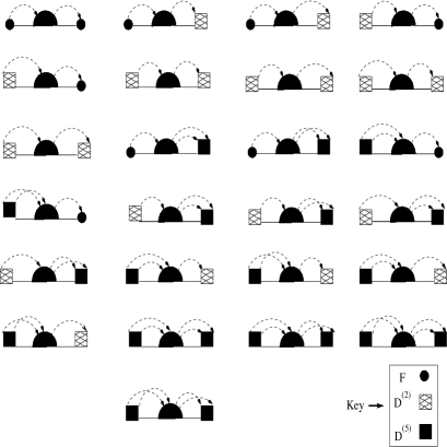
Figure 2: Structure of the skeleton diagrams for the self-energy

In our earlier paper am2 we had developed a multiple scattering picture for the configuration averaged Green function. The idea is very similar to that of Edwards and Langer ed ; la in the context of purely diagonal disorder. The scattering vertices associated with the terms in the ”perturbing” part of the dynamical matrix : $\widetilde{\mathbf{D}}_{1}$ are shown in Fig. 1.

The end point of that formulation was the derivation of a Dyson equation :

$$\ll{\mathbf{G}}\gg={\mathbf{g}}+{\mathbf{g}}\ {\mathbf{\Sigma}}\ll{\mathbf{G}}\gg.$$

For homogeneous disorder we have shown earlier that we have translational symmetry in the full augmented space gdma . We can then take Fourier transform of the above equation to get

$$\ll\mathbf{G}({\mathbf{k}}\ ,E)\gg=\mathbf{g}({\mathbf{k}}\ ,E)+\mathbf{g}({\mathbf{k}}\ ,E)\ \mathbf{\Sigma}({\mathbf{k}}\ ,E)\ \ll\mathbf{G}({\mathbf{k}}\ ,E)\gg.$$

The diagrams for the self-energy are skeleton diagrams which have the structure as shown in Fig. 2. Each of the 25 different diagram starts with any one of F, D⁽²⁾ or D⁽⁵⁾ and the central dark semicircle represents all possible arrangements of scattering vertices to all orders.

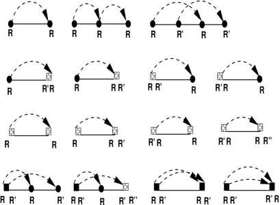
Figure 3: Details of some skeleton diagrams for the self-energy

Let us now examine some specific Edwards-Langer scattering diagrams, in some detail, in order to understand their physical significance and relation to mean-field approximations. The first three diagrams on the first row of Fig 3 arise because of purely diagonal disorder in mass. Of these the first two diagrams describe self-energy corrections to the VCA propagator because of configurations fluctuations at a single site. These diagrams are closely related to the diagrammatic treatment discussed by Leath leath-diag . Referring to that earlier work, we note that these diagrams are explicitly included in the 1CPA. The self-energy arising out of such diagrams is site-diagonal, or k-independent in reciprocal space. The third diagram is the smallest order diagram of this type which describes joint configuration fluctuations of two distinct sites. These type of diagrams take us beyond the 1CPA. For the 1CPA we ignore these fourth order diagrams, and all higher order diagrams, to all orders, describing joint configuration fluctuations of more than two sites. Within this approximation, the first inaccurate moment of the density of states is of order eight. If we include diagrams to all orders which describe joint configuration fluctuations of two sites we are lead to the 2CPA. This has been described in detail in the work of Aiyer et.al. aekl and Nickel and Krummhansl nk .

The diagrams in the second row of Fig 3 describe self-energy corrections due to configuration fluctuations at a single site for both diagonal (mass) and off-diagonal (force-constant) disorders. The first and the third diagrams lead to a diagonal self-energy, while the second and fourth diagrams lead to an off-diagonal contribution to the self-energy in real space. For off-diagonal disorder even these second order diagrams can lead to off-diagonal (real space) or k-dependent (reciprocal space) self-energy. Ignoring these contributions ( to all orders) will lead to a 1CPA type approximation where even the fourth moment of the density of states will be inaccurate. This had been noted earlier for 1CPA in off-diagonal disorder problems. The diagrams in row three of Fig 3 are very similar contributions from configuration fluctuations at a single site but arising out of pure off-diagonal disorder.

The diagrams on the last row of Fig 3 describe self-energy contributions coming from joint fluctuations of two sites arising out of off-diagonal disorder. All such diagrams take us beyond the 1CPA and some of them contribute to a self-energy which is off-diagonal (real space) or k-dependent (reciprocal space).

The formal summing up, to infinite order, of diagrams which involve configuration fluctuations involving single sites has been discussed by Leath leath-diag . This leads to the 1CPA and within this approximation the first inaccuracy occurs in the eighth moment of the averaged density of states. Nickel and Krummhansl nk have discussed in detail how to sum up, to infinite order, diagrams which also include joint configuration fluctuations of two sites. It is clear from this paper that any generalization of a purely diagrammatic treatment of joint multi-site configuration fluctuations is a very difficult task indeed. However, a recursion based calculation of the self-energy, as proposed by us in our earlier paper am2 , includes the contribution of such diagrams. We note that if we calculate the continued fraction coefficients exactly up to n steps then all the first 2n moments of the density of states are exact. In addition the Beer-Pettifor terminator ensures both the herglotz analytic properties of the Green function and accuracy of the asymptotic moments. As in our earlier papers am1 ; am2 , therefore, we propose the augmented space recursion as an alternative method for the calculation of averaged Green functions including effects of joint multi-site configuration fluctuations.

III.3 Generalized scattering diagrams for the averaged thermal conductivity

We now go back to equation (5) and discuss the configuration averaging of the two-particle Green functions of the kind $\kappa(z_{1},z_{2})$. The augmented space theorem immediately implies that

$$\ll{\mathbf{\kappa}}(z_{1},z_{2})\gg\phantom{xxxxxxxxxxxxxxxxxxxxxxxxxxxxxx}$$

$$\phantom{x}=\int\frac{d^{3}{\mathbf{k}}\ }{8\pi^{3}}\ \left\langle\{\emptyset\}\left|\ \mbox{Tr}\left[\rule{0.0pt}{11.38109pt}\right.\widetilde{\mathbf{S}}\widetilde{\mathbf{G}}({\mathbf{k}}\ ,z_{1})\ \widetilde{\mathbf{S}}\widetilde{\mathbf{G}}({\mathbf{k}}\ ,z_{2})\right]\ \left.\rule{0.0pt}{11.38109pt}\right|\{\emptyset\}\right\rangle$$

In real space the random expression $\widehat{\mathbf{S}}$ for a binary alloy can take the values $\widehat{\mathbf{S}}^{AA}$, $\widehat{\mathbf{S}}^{AB}$, $\widehat{\mathbf{S}}^{BA}$ or $\widehat{\mathbf{S}}^{BB}$ with probabilities $x^{2}$ , $xy$, $yx$ and $y^{2}$ respectively. We may rewrite the current $\widehat{\mathbf{S}}_{R\alpha,R^{\prime}\beta}$ as

$$\widehat{\mathbf{S}}_{R\alpha,R^{\prime}\beta}=\widehat{\mathbf{S}}^{AA}_{R\alpha,R^{\prime}\beta}\ n_{R}\ n_{R^{\prime}}+\widehat{\mathbf{S}}^{AB}_{R\alpha,R^{\prime}\beta}\ n_{R}\ (1-n_{R^{\prime}})+$$

$$\enskip+\enskip\widehat{\mathbf{S}}^{BA}_{R\alpha,R^{\prime}\beta}\ (1-n_{R})\ n_{R^{\prime}}+\widehat{\mathbf{S}}^{BB}_{R\alpha,R^{\prime}\beta}\ (1-n_{R})(1-n_{R^{\prime}}).$$

Following the same procedure as for the single particle Green functions we get

$$\widetilde{{\mathbf{S}}} = \sum_{R\alpha}\sum_{R^{\prime}\alpha^{\prime}}\left[\rule{0.0pt}{11.38109pt}\ll\widehat{{\mathbf{S}}}\gg_{R\alpha,R^{\prime}\alpha^{\prime}}\widetilde{I}\otimes T_{RR^{\prime}}+{{\mathbf{S}}}^{(1)}_{R\alpha,R^{\prime}\alpha^{\prime}}\right.$$

$$\left.\left({p}^{\downarrow}_{R}+{p}^{\downarrow}_{R^{\prime}}\right)\otimes T_{RR^{\prime}}+{{\mathbf{S}}}^{(2)}_{R\alpha,R^{\prime}\alpha^{\prime}}\left({\cal T}^{\uparrow\downarrow}_{R}+{\cal T}^{\uparrow\downarrow}_{R^{\prime}}\right)\otimes T_{RR^{\prime}}\right.$$

$$\left.+{{\mathbf{S}}}^{(3)}_{R\alpha,R^{\prime}\alpha^{\prime}}p^{\downarrow}_{R}\otimes p^{\downarrow}_{R^{\prime}}\otimes T_{RR^{\prime}}+{{\mathbf{S}}}^{(4)}_{R\alpha,R^{\prime}\alpha^{\prime}}\left(p^{\downarrow}_{R}\otimes{\cal T}^{\uparrow\downarrow}_{R^{\prime}}+\right.\right.$$

$$\left.\left.p^{\downarrow}_{R^{\prime}}\otimes{\cal T}^{\uparrow\downarrow}_{R}\right)\otimes T_{RR^{\prime}}+{{\mathbf{S}}}^{(5)}_{R\alpha,R^{\prime}\alpha^{\prime}}{\cal T}^{\uparrow\downarrow}_{R}\otimes{\cal T}^{\uparrow\downarrow}_{R^{\prime}}\otimes T_{RR^{\prime}}\right],$$

where

$${\mathbf{S}}^{(1)} = (y-x)\ \widehat{{\mathbf{S}}}^{(1)},\ \ {\mathbf{S}}^{(2)}=\sqrt{xy}\ \widehat{{\mathbf{S}}}^{(1)},$$

$${\mathbf{S}}^{(3)} = (y-x)^{2}\ \widehat{{\mathbf{S}}}^{(2)},\ \ {\mathbf{S}}^{(4)}=\sqrt{xy}\ (y-x)\ \widehat{{\mathbf{S}}}^{(2)},$$

$${\mathbf{S}}^{(5)} = xy\ \widehat{{\mathbf{S}}}^{(2)}.$$

and

$$\widehat{{\mathbf{S}}}^{(1)}_{R\alpha,R^{\prime}\beta} = x\left(\widehat{{\mathbf{S}}}^{AA}_{R\alpha,R^{\prime}\beta}-\widehat{{\mathbf{S}}}^{AB}_{R\alpha,R^{\prime}\beta}\right)-y\left(\widehat{{\mathbf{S}}}^{BB}_{R\alpha,R^{\prime}\beta}-\right.$$

$$\left.\widehat{{\mathbf{S}}}^{BA}_{R\alpha,R^{\prime}\beta}\right)$$

$$\widehat{{\mathbf{S}}}^{(2)}_{R\alpha,R^{\prime}\beta} = \widehat{{\mathbf{S}}}^{AA}_{R\alpha,R^{\prime}\beta}+\widehat{{\mathbf{S}}}^{BB}_{R\alpha,R^{\prime}\beta}-\widehat{{\mathbf{S}}}^{AB}_{R\alpha,R^{\prime}\beta}-\widehat{{\mathbf{S}}}^{BA}_{R\alpha,R^{\prime}\beta}.$$

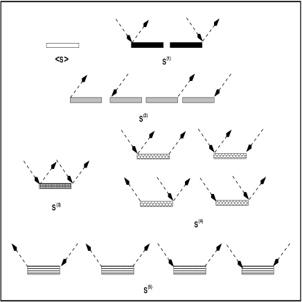
Figure 4: The scattering vertices associated with the random current terms

Equation (LABEL:eq12) is very similar to (16), which shows the terms arising in augmented space due to the disorder in the dynamical matrix. Fig. 4 shows the sixteen different scattering vertices arising out of Eq. (LABEL:eq12). We may compare the scattering vertices arising out of disorder in the current term with those that arise from disorder in the dynamical matrix shown in Fig. 1. We note the close similarity between them leading to both terms which arise because of configuration fluctuations at a single site and also two sites.

Note that the averaging of $\kappa(z_{1},z_{2})$ involves averaging of a product of four terms two involving the thermal currents $S$ and two Green functions. These random functions are not independent, but are all intrinsic functions of the random occupation variables $n_{R}$. The average of the product is therefore not the product of the averages.

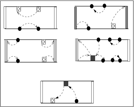
Figure 5: Different classes of scattering diagrams for the thermal conductivity

Let us now examine the various classes of scattering diagrams. The simplest one is the type shown on the top left of Fig 5. These diagrams involve two averaged current terms and two propagators decorated with scattering diagrams in all possible ways. The contribution of such a term (the zero-th order term) is then,

$$\kappa_{(0)}(z_{1},z_{2}) = \int\frac{\displaystyle d^{3}{\mathbf{k}}\ }{\displaystyle 8\pi^{3}}\ \mathrm{Tr}\left[\rule{0.0pt}{11.38109pt}\ll{\mathbf{S}}\gg\ll{\mathbf{G}}({\mathbf{k}}\ ,z_{1})\gg\right.$$

$$\left.\rule{0.0pt}{11.38109pt}\ll{\mathbf{S}}\gg{\mathbf{G}}({\mathbf{k}}\ ,z_{2})\gg\right]$$

The next type of scattering diagrams are the types shown on the top right of Fig 5. These diagrams connect a current term to a propagator. The first type of scattering diagrams are those in which disorder lines do not connect the two phonon propagators. Fig 6 shows the general structure of such diagrams. It is clear from the figure that these diagrams renormalize the current terms. Fig 7 shows all possible renormalized currents arising out of diagrams of this class.

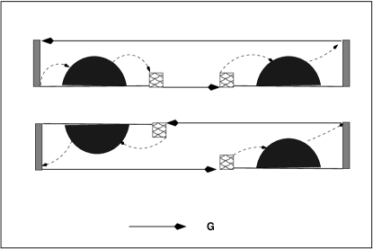
Figure 6: Two examples of scattering diagrams where no disorder line joins the two phonon propagators

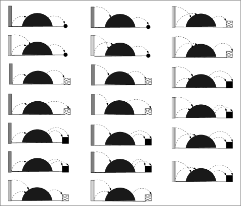
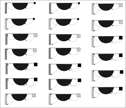
Figure 7: Scattering diagrams contributing to effective heat current

In our earlier paper on optical conductivity sm we had shown that this type of diagrams provide the predominant disorder correction to the current terms in the electronic problem. If we compare them with the diagrams for the self energy (Fig. 2) we note that for the diagrams in the left panel of Fig. 7, the only difference is that the leftmost scattering vertex is replaced by a very similar current term. Similarly the diagrams on the right panel are the same as the self-energy diagrams except that the last vertex is replaced by a very similar current term. In all these diagrams of Fig. 7 the left and rightmost diagonal term similar to the vertex F of Fig. 1 is of course missing. We may then go on to write

$$\Delta{{\mathbf{S}}}_{1}({\mathbf{k}}\ )(z_{1},z_{2})=\phantom{xxxxxxxxxxXXXXXXXX}$$

$$2\left(\rule{0.0pt}{8.53581pt}{{\mathbf{S}}}^{(2)}({\mathbf{k}}\ )+{{\mathbf{S}}}^{(5)}({\mathbf{k}}\ )\right)\left[\rule{0.0pt}{9.95845pt}\Delta{({\mathbf{k}}\ ,z_{1})}\right]^{-1}{\mathbf{\Sigma}}({\mathbf{k}}\ ,z_{1})+$$

$${\mathbf{\Sigma}}({\mathbf{k}}\ ,z_{2})\left[\rule{0.0pt}{9.95845pt}\Delta{({\mathbf{k}}\ ,z_{2})}\right]^{-1}2\left(\rule{0.0pt}{8.53581pt}{{\mathbf{S}}}^{(2)}({\mathbf{k}}\ )+{{\mathbf{S}}}^{(5)}({\mathbf{k}}\ )\right),\phantom{x}$$

Figure 8: More scattering diagrams contributing to effective current

where

$$\Delta{({\mathbf{k}}\ ,z)}={\mathbf{F}}z^{2}+2{\mathbf{D}}^{(2)}({\mathbf{k}}\ )+2{\mathbf{D}}^{(5)}({\mathbf{k}}\ ).$$

The next most dominant disorder corrections come from the diagrams shown in the middle row of Fig 5. A general such diagram is shown in Fig. 8. These diagram connect one current term to two propagators. These diagrams also renormalize this current term. Again looking at these diagrams we note that they are also related to a self-energy diagrams with vertices at both ends replaced by currents. We therefore may write

$$\Delta{{\mathbf{S}}}_{2}({\mathbf{k}}\ )(z_{1},z_{2})=\phantom{XXXXXXXXXXXXXXXXX}$$

$${\mathbf{\Sigma}}({\mathbf{k}}\ ,z_{2})\left[\rule{0.0pt}{9.95845pt}\Delta{({\mathbf{k}}\ ,z_{2})}\right]^{-1}{\mathbf{S}}^{(5)}({\mathbf{k}}\ )\left[\rule{0.0pt}{9.95845pt}\Delta{({\mathbf{k}}\ ,z_{1})}\right]^{-1}{\mathbf{\Sigma}}({\mathbf{k}}\ ,z_{1})$$

$$+{\mathbf{\Sigma}}({\mathbf{k}}\ ,z_{1})\left[\rule{0.0pt}{9.95845pt}\Delta{({\mathbf{k}}\ ,z_{1})}\right]^{-1}{\mathbf{S}}^{(5)}({\mathbf{k}}\ )\left[\rule{0.0pt}{9.95845pt}\Delta{({\mathbf{k}}\ ,z_{2})}\right]^{-1}{\mathbf{\Sigma}}({\mathbf{k}}\ ,z_{2}).$$

The effective current is then given by

$${{\mathbf{S}}}_{\mathrm{eff}}({\mathbf{k}}\ ,z_{1},z_{2})=\phantom{XXXXXXXXXXXXXX}$$

$$\ll\widehat{{\mathbf{S}}}({\mathbf{k}}\ )\gg+\Delta{{\mathbf{S}}}_{1}({\mathbf{k}}\ )(z_{1},z_{2})+\Delta{{\mathbf{S}}}_{2}({\mathbf{k}}\ )(z_{1},z_{2}).$$ (20)

In our earlier paper sm on a similar electronic problem we have argued that these are the dominant disorder corrections to the current term. With these corrections we obtain

$$\kappa_{(1)}(z_{1},z_{2}) = \int\frac{d^{3}{\mathbf{k}}\ }{8\pi^{3}}\ \mathrm{Tr}\left[\rule{0.0pt}{11.38109pt}{{\mathbf{S}}}_{\mathrm{eff}}({\mathbf{k}}\ ,z_{1},z_{2})\ll{\mathbf{G}}({\bf k},z_{1})\gg\right.$$ (21)

$$\left.{{\mathbf{S}}}_{\mathrm{eff}}^{\dagger}({\mathbf{k}}\ ,z_{1},z_{2})\ll{\mathbf{G}}({\bf k},z_{2})\gg\right].$$

Since averaging the thermal conductivity involves averaging the product of two propagators and two current terms, we may physically understand the different terms in Fig. 5 in the following way : the top left diagram is related to the product of the averages. The term on the top row to the right is related to a pair of joint averages of one propagator and one current term. The diagrams on the second row are related to the product of the average of one current and the average of the product of two propagators and a current. The bottom most diagram is related to the product of two averaged currents and the average of the product of two propagators.

III.4 Averaged thermal diffusivity

For a harmonic solid, a temperature independent mode diffusivity $D_{\gamma}$ is defined as

$$D^{\mu\nu}_{\gamma}({\mathbf{k}}\ )=\pi\sum_{\gamma^{\prime}\neq\gamma}\frac{1}{\omega_{{\mathbf{k}}\ \gamma}^{2}}{\mathbf{S}}^{\mu}_{\gamma\gamma^{\prime}}({\mathbf{k}}\ ){\mathbf{S}}^{\nu}_{\gamma^{\prime}\gamma}({\mathbf{k}}\ )\ \delta(\omega_{{\mathbf{k}}\ \gamma}-\omega_{{\mathbf{k}}\ \gamma^{\prime}}).$$

This is an intrinsic property of the $\gamma$-th normal mode and provides an unambiguous criterion for localization.

The averaged thermal diffusivity (averaged over modes) is then given by

$${\bf D}^{\mu\nu}(\omega) = \frac{\displaystyle\int\frac{d^{3}{\mathbf{k}}\ }{8\pi^{3}}\sum_{\gamma}D^{\mu\nu}_{\gamma}({\mathbf{k}}\ )\delta(\omega-\omega_{{\mathbf{k}}\ \gamma})}{\displaystyle\int\frac{d^{3}{\mathbf{k}}\ }{8\pi^{3}}\sum_{\gamma}\delta(\omega-\omega_{{\mathbf{k}}\ \gamma})}$$ (22)

$$= \frac{D^{\mu\nu}_{tot}(\omega)}{{\displaystyle\int\frac{d^{3}{\mathbf{k}}\ }{8\pi^{3}}\sum_{\gamma}\delta(\omega-\omega_{{\mathbf{k}}\ \gamma})}}.$$

Assuming isotropy of the response, we can rewrite the numerator of above equation as

$$D^{\mu\mu}_{tot}(\omega) = \pi\int d\omega^{\prime}\int\frac{d^{3}{\mathbf{k}}\ }{8\pi^{3}}\sum_{\gamma}\sum_{\gamma^{\prime}}\widehat{S}^{\mu}_{\gamma\gamma^{\prime}}({\mathbf{k}}\ )\widehat{S}^{\mu}_{\gamma^{\prime}\gamma}({\mathbf{k}}\ )$$

$$\delta(\omega^{\prime}-\omega_{{{\mathbf{k}}\ }\gamma^{\prime}})\delta(\omega_{{{\mathbf{k}}\ }\gamma}-\omega^{\prime})\delta(\omega-\omega_{{{\mathbf{k}}\ }\gamma}),$$

where

$$\widehat{S}^{\mu}_{\gamma\gamma^{\prime}}({\mathbf{k}}\ )\ =\ \frac{1}{\omega_{{\mathbf{k}}\ \gamma}}{\mathbf{S}}^{\mu}_{\gamma\gamma^{\prime}}({\mathbf{k}}\ ).$$

We may again rewrite the above equation for $D_{tot}$ as

$$D^{\mu\mu}_{tot}(\omega) = \frac{1}{\pi^{2}}\int d\omega^{\prime}\int\frac{d^{3}{\mathbf{k}}\ }{8\pi^{3}}\mbox{Tr}\left[\Im m\{{\mathbf{G}}({\mathbf{k}}\ ,\omega^{\prime})\}\widehat{\mathbf{S}}^{\mu}({\mathbf{k}}\ )\right.$$

$$\left.\Im m\{{\mathbf{G}}({\mathbf{k}}\ ,\omega^{\prime})\}\widehat{\mathbf{S}}^{\mu}({\mathbf{k}}\ )\Im m\{{\mathbf{G}}({\mathbf{k}}\ ,\omega)\}\right].$$

The averaged thermal diffusivity can then be expressed as ( for an isotropic response )

$${\mathbf{D}}(\omega) = \frac{1}{3}\sum_{\mu}D^{\mu\mu}(\omega)$$ (23)

$$= \frac{\pi}{3}\frac{\sum_{\mu}{\mathbf{D}}_{tot}^{\mu\mu}(\omega)}{\displaystyle\int\frac{d^{3}{\mathbf{k}}\ }{8\pi^{3}}\mbox{Tr}\left[\Im m\{{\mathbf{G}}({\mathbf{k}}\ ,\omega)\}\right]}.$$

For disordered material, we shall be interested as before in obtaining the configuration averaged thermal diffusivity. We have already discussed the configuration averaging of the two particle Green function using scattering diagram technique in Sec. III(C). It has been found that the net effect is to replace the current terms by an effective heat current ${\mathbf{S}}_{eff}({\mathbf{k}}\ ,z_{1},z_{2})$. The effective current is a sum of average current and the terms arising out of the disorder correction. As in the case of optical conductivity calculation sm , it will be shown that the overall contribution of disorder correction terms to the thermal conductivity is very small as compared to the average current $\ll\widehat{\mathbf{S}}({\mathbf{k}}\ )\gg$. Keeping in mind this effect of disorder correction terms to the heat current, the configuration averaged thermal diffusivity can be expressed (to a 1st order approximation) in the form

$$\ll{\mathbf{D}}(\omega)\gg=\frac{\pi}{3}\frac{\sum_{\mu}\ll{\mathbf{D}}_{tot}^{\mu\mu}(\omega)\gg}{\displaystyle\int\frac{d^{3}{\mathbf{k}}\ }{8\pi^{3}}\mbox{Tr}\left[\Im m\ll{\mathbf{G}}({\mathbf{k}}\ ,\omega)\gg\right]},$$ (24)

where

$$\ll D^{\mu\mu}_{tot}(\omega)\gg\ \simeq\ \frac{1}{\pi^{2}}\int d\omega^{\prime}\int\frac{d^{3}{\mathbf{k}}\ }{8\pi^{3}}\mbox{Tr}\left[\rule{0.0pt}{11.38109pt}\Im m\ll{\mathbf{G}}({\mathbf{k}}\ ,\omega^{\prime})\gg\right.$$

$$\left.\ll\widehat{\mathbf{S}}^{\mu}({\mathbf{k}}\ )\ \Im m\ \{{\mathbf{G}}({\mathbf{k}}\ ,\omega^{\prime})\}\ \widehat{\mathbf{S}}^{\mu}({\mathbf{k}}\ )\ \rule{0.0pt}{11.38109pt}\Im m\{{\mathbf{G}}({\mathbf{k}}\ ,\omega)\}\gg\right].$$

(25)

III.5 The vertex correction

We shall now examine the scattering diagrams we have left out, namely, those in which disorder lines connect both the propagators directly. One such diagram is the bottom-most diagram shown in Fig 5. These lead to vertex corrections due to correlated propagation. In general we obtain a Bethe-Salpeter equation for the averaged two-particle propagator. This is diagrammatically shown in Fig 9.

Figure 9: The Bethe-Salpeter equation for the thermal conductivity

To obtain the vertex correction, shown in Fig 9, we shall consider only a special class of vertex diagrams in this communication : namely the scattering diagrams which are built out of repeated vertices. These are called the ladder diagrams and can be summed up to all orders. This is the disorder scattering version of the random phase approximation (RPA).

A few amongst all the possible scattering diagrams for the ladder type of vertex corrections involving the vertices ${\mathbf{B}}$, ${\mathbf{F}}$, ${\mathbf{D}}^{(1)}$, ${\mathbf{D}}^{({2})}$, ${\mathbf{D}}^{({3})}$, ${\mathbf{D}}^{({4})}$, ${\mathbf{D}}^{({5})}$ are as shown in Fig. 10

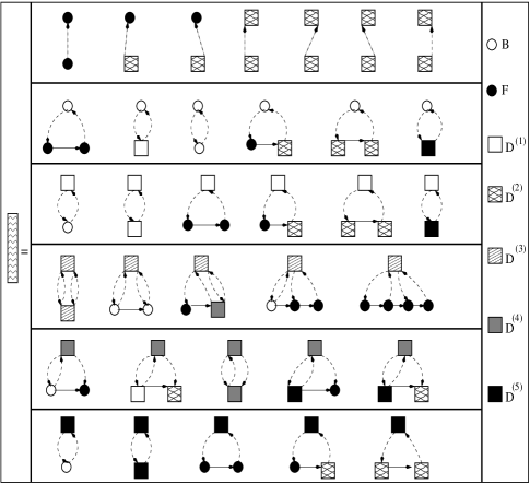
Figure 10: The scattering diagrams for the ladder type of vertex correction.

The contribution of diagrams from the first line of Fig. 10 in the four legged vertex (shown in the extreme left column of the same figure) is given by

$$\left(W^{\gamma\delta}_{\alpha\beta}\right)_{\mbox{1st line}}=\phantom{xxxxxxxxxxxxxxxxxxxxxx}$$

$$(z_{1}z_{2})^{2}\ F_{\alpha}F_{\gamma}\ \delta_{\alpha\beta}\delta_{\gamma\delta}+2z_{2}^{2}\ D^{(2)}_{\alpha\beta}\ F^{\gamma}\ \delta_{\gamma\delta}$$

$$+2z_{1}^{2}\ D^{(2)}_{\gamma\delta}\ F^{\alpha}\ \delta_{\alpha\beta}+4D^{(2)}_{\alpha\beta}\ D^{(2)}_{\gamma\delta}.$$ (26)

The contribution of the second line of diagrams and all those obtained from them by simple reflection operations about the vertical and horizontal directions is given by

$$\left(W^{\gamma\delta}_{\alpha\beta}\right)_{\mbox{2nd line}}=({z_{1}}^{2}z_{2})^{2}\left[\sum_{\nu^{\prime}\nu^{\prime\prime}}(F_{\alpha\nu^{\prime}}\delta_{\alpha\nu^{\prime}})\ G_{R\nu^{\prime},R\nu{\prime\prime}}\ (F_{\nu^{\prime\prime}\beta}\delta_{\nu^{\prime\prime}\beta})\right](B_{\nu\delta}\delta_{\nu\delta})+({z_{1}}{z_{2}}^{2})^{2}(B_{\alpha\beta}\delta_{\alpha\beta})$$

$$\times\left[\sum_{\nu^{\prime}\nu^{\prime\prime}}(F_{\nu\nu^{\prime}}\delta_{\nu\nu^{\prime}})\ G_{R\nu^{\prime},R\nu{\prime\prime}}\ (F_{\nu^{\prime\prime}\delta}\delta_{\nu^{\prime\prime}\delta})\right]+2\left[D^{(1)}_{\alpha\beta}({z_{2}}^{2}B_{\nu\delta}\delta_{\nu\delta})\right]+2\left[({z_{1}}^{2}B_{\alpha\beta}\delta_{\alpha\beta})D^{(1)}_{\nu\delta}\right]+({z_{1}}^{2}B_{\alpha\beta}\delta_{\alpha\beta})({z_{2}}^{2}B_{\nu\delta}\delta_{\nu\delta})$$

$$+\ 2\left[\sum_{\nu^{\prime}\nu^{\prime\prime}}({z_{1}}^{2}F_{\alpha\nu^{\prime}}\delta_{\alpha\nu^{\prime}})\ G_{R\nu^{\prime},R\nu{\prime\prime}}\ D^{(2)}_{\nu^{\prime\prime}\beta}\right]({z_{2}}^{2}B_{\nu\delta}\delta_{\nu\delta})+2\ ({z_{1}}^{2}B_{\alpha\beta}\delta_{\alpha\beta})\left[\sum_{\nu^{\prime}\nu^{\prime\prime}}({z_{2}}^{2}F_{\nu\nu^{\prime}}\delta_{\nu\nu^{\prime}})\ G_{R\nu^{\prime},R\nu{\prime\prime}}\ D^{(2)}_{\nu^{\prime\prime}\delta}\right]$$

$$+\ 2\left[\sum_{\nu^{\prime}\nu^{\prime\prime}}D^{(2)}_{\alpha\nu^{\prime}}\ G_{R\nu^{\prime},R\nu{\prime\prime}}\ ({z_{1}}^{2}F_{\nu^{\prime\prime}\beta}\delta_{\nu^{\prime\prime}\beta})\right]({z_{2}}^{2}B_{\nu\delta}\delta_{\nu\delta})+2\ ({z_{1}}^{2}B_{\alpha\beta}\delta_{\alpha\beta})\left[\sum_{\nu^{\prime}\nu^{\prime\prime}}D^{(2)}_{\nu\nu^{\prime}}\ G_{R\nu^{\prime},R\nu{\prime\prime}}\ ({z_{2}}^{2}F_{\nu^{\prime\prime}\delta}\delta_{\nu^{\prime\prime}\delta})\right]$$

$$+\ 4\left[\sum_{\nu^{\prime}\nu^{\prime\prime}}D^{(2)}_{\alpha\nu^{\prime}}\ G_{R\nu^{\prime},R\nu{\prime\prime}}\ D^{(2)}_{\nu^{\prime\prime}\beta}\right]({z_{2}}^{2}B_{\nu\delta}\delta_{\nu\delta})+4({z_{1}}^{2}B_{\alpha\beta}\delta_{\alpha\beta})\left[\sum_{\nu^{\prime}\nu^{\prime\prime}}D^{(2)}_{\nu\nu^{\prime}}\ G_{R\nu^{\prime},R\nu{\prime\prime}}\ D^{(2)}_{\nu^{\prime\prime}\delta}\right]\phantom{XXXXXXXX}$$

$$+\ D^{(5)}_{\alpha\beta}({z_{2}}^{2}B_{\nu\delta}\delta_{\nu\delta})+({z_{1}}^{2}B_{\alpha\beta}\delta_{\alpha\beta})D^{(5)}_{\nu\delta}.\phantom{XXXXXXXXXXXXXXXXXXXXXXXXXXXX}$$ (27)

The contribution of rest of the diagrams may be obtained in exactly the same way.

Figure 11: The structure of infinite series of ladder diagrams.

If the sum of all possible scattering diagrams contributing to the four legged vertex shown in the left column of Fig. 10 is denoted by $W_{\alpha\beta}^{\nu\delta}$, then the infinite series of ladder diagrams shown in Fig. 11 may be directly summed up as follows : If we define

$${\mathbf{\Gamma}}(z_{1},z_{2}) = \int_{BZ}\frac{d^{3}{\mathbf{k}}\ }{8\pi^{3}}\ {\mathbf{G}}({\mathbf{k}}\ ,z_{2})\widehat{{\mathbf{S}}}^{\mathrm{eff}}({\mathbf{k}}\ ,z_{1},z_{2}){\mathbf{G}}({\mathbf{k}}\ ,z_{1}),$$

$$\widehat{\mathbf{\Gamma}}(z_{1},z_{2}) = \int_{BZ}\frac{d^{3}{\mathbf{k}}\ }{8\pi^{3}}\ {\mathbf{G}}({\mathbf{k}}\ ,z_{1})\widehat{{\mathbf{S}}}^{\mathrm{eff}}({\mathbf{k}}\ ,z_{1},z_{2})^{\dagger}\ {\mathbf{G}}({\mathbf{k}}\ ,z_{2}),$$

$${\mathbf{\Theta}}_{\alpha\beta}^{\gamma\delta}(z_{1},z_{2}) = \int_{BZ}\frac{d^{3}{\mathbf{k}}\ }{8\pi^{3}}\ G_{\alpha\beta}({\mathbf{k}}\ ,z_{1})\ G_{\gamma\delta}({\mathbf{k}}\ ,z_{2}),$$

Then

$${\mathbf{\Lambda}}(z_{1},z_{2}) = {\mathbf{W}}+{\mathbf{W}}{\mathbf{\Theta}}{\mathbf{W}}+{\mathbf{W}}{\mathbf{\Theta}}{\mathbf{W}}{\mathbf{\Theta}}{\mathbf{W}}+\ldots$$

$$= {\mathbf{W}}(z_{1},z_{2})\left(\rule{0.0pt}{11.38109pt}{\mathbf{I}}-{\mathbf{\Theta}}(z_{1},z_{2}){\mathbf{W}}(z_{1},z_{2})\right)^{-1}.$$

Thus we get

$$\ll\Delta\kappa(z_{1},z_{2})^{\mathrm{l}adder}\gg\phantom{XXXXXXXXXXXXX}$$

$$=\sum_{\alpha\beta}\sum_{\nu\delta}{\mathbf{\Gamma}}^{\alpha}_{\beta}(z_{1},z_{2})\ {\mathbf{\Lambda}}_{\beta\delta}^{\alpha\nu}(z_{1},z_{2})\ \widehat{\mathbf{\Gamma}}^{\nu}_{\delta}(z_{1},z_{2})\phantom{xxx}$$

$$=\mathrm{Tr}\left[\rule{0.0pt}{11.38109pt}{\mathbf{\Gamma}}(z_{1},z_{2})\otimes\widehat{\mathbf{\Gamma}}(z_{1},z_{2})\ {\mathbf{\odot}}\ {\mathbf{\Lambda}}(z_{1},z_{2})\right].\phantom{xxxx}$$ (29)

The configuration average of the two-particle green function is then given by

$$\ll\kappa(z_{1},z_{2})\gg=\ll\kappa_{(1)}(z_{1},z_{2})\gg\ +\ \ll\Delta\kappa(z_{1},z_{2})^{\mathrm{l}adder}\gg$$ (30)

IV DETAILS OF NUMERICAL IMPLEMENTATION

Although we have used the scattering diagrammatic technique to analyze the effects of disorder scattering on the thermal conductivity and obtain relation between the effective current and self-energy, we shall not use this approach to actually numerically obtain the thermal conductivity for a real alloy system. If we look at the earlier sections we note that what we need to obtain are essentially the configuration averaged Green matrices and the matrix self-energies. For this we shall use the augmented space block-recursion am2 and also the Brillouin zone integration scheme developed by us earlier smj . In this section we shall briefly discuss the two techniques.

IV.1 Block Recursion

As is clear from the expression of configuration averaged lattice thermal conductivity and thermal diffusivity that the numerical evaluation of these quantities require the full Green matrix and the self energy matrix instead of their diagonal elements alone.

In a recent communication am2 , we have already described the block recursion technique, which calculates the entire green matrix and the self energy matrix. For the sake of completeness, we shall describe in brief the salient features of the technique. In the block recursion, we start from a matrix basis of the form $\{\Phi^{(n)}_{J,\alpha\beta}\}$, where $J$ is the discrete labeling of the augmented space states and the $\alpha,\beta$ labels Cartesian directions.

For a reciprocal space based calculation (as in the present case) we start with

$$\Phi^{(1)}_{J,\alpha\beta}\ =\ U_{\alpha\beta}^{(1)}\ \delta_{J,1}+U_{\alpha\beta}^{(2)}\ \delta_{J,2},$$

where

$U_{\alpha\beta}^{(1)}=\frac{\displaystyle A(m^{-1/2})}{\displaystyle\left[\rule{0.0pt}{5.69054pt}A(m^{-1})\right]^{1/2}}\ \delta_{\alpha\beta},\ \ \ U_{\alpha\beta}^{(2)}=\frac{\displaystyle F(m^{-1/2})}{\displaystyle\left[\rule{0.0pt}{5.69054pt}A(m^{-1})\right]^{1/2}}\ \delta_{\alpha\beta}$,

with

$A(X)=(xX_{A}+yX_{B}),\ \ \ F(X)=(y-x)(X_{A}-X_{B})$.

The remaining terms in the basis are recursively obtained from

$$\sum_{\beta^{\prime}}\Phi^{(n+1)}_{J,\alpha\beta^{\prime}}B^{(n+1)\dagger}_{\beta^{\prime}\beta} = \sum_{J^{\prime}}\sum_{\beta^{\prime}}\widetilde{H}_{J\alpha,J^{\prime}\beta^{\prime}}\Phi^{(n)}_{J^{\prime},\beta^{\prime}\beta}-$$

$$\sum_{\beta^{\prime}}\Phi^{(n)}_{J,\alpha\beta^{\prime}}A^{(n)}_{\beta^{\prime}\beta}-\sum_{\beta^{\prime}}\Phi^{(n-1)}_{J,\alpha\beta^{\prime}}B^{(n)}_{\beta^{\prime}\beta},$$

where $\widetilde{H}$ is the lattice vibrational Hamiltonian (under harmonic approximation) in the augmented space. We then use the Gram-Schmidt orthonormalization method to keep track of orthogonality condition among the various columns of $\Phi^{(n)}_{J,\alpha\beta}$ and hence to calculate the matrix coefficient ${\bf B}^{(n+1)}$. Since the Hamiltonian in this new basis is block tri-diagonal, so the green matrix can be expressed as a matrix continued fraction in terms of the coefficients ${{\bf A}^{n},{\bf B}^{(n+1)}}$ as follows :

$${\mathbf{G}}^{(n)} = \left[\rule{0.0pt}{11.38109pt}w^{2}\ {\mathbf{I}}-{\mathbf{A}}^{(n)}-{\mathbf{B}}^{(n+1)\dagger}\ {\mathbf{G}}^{(n+1)}\ {\mathbf{B}}^{(n+1)}\right]^{-1},$$

$$\ll{\mathbf{G}}\gg = {\mathbf{G}}^{(1)}.$$ (31)

We calculate the matrix coefficients up to a $n=N_{0}$ and approximate at coefficients $>N_{0}$ by A and B.We then write for a $N\gg N_{0}$,

$${\mathbf{G}}^{(N)}\ =\ \left[\rule{0.0pt}{11.38109pt}(w^{2}-i\delta){\mathbf{I}}\right]^{-1}$$

and then iterate

$$G^{(n)}=\left[\rule{0.0pt}{11.38109pt}w^{2}{\mathbf{I}}\ -\ {\mathbf{A}}\ -\ {\mathbf{B}}^{\dagger}\ {\mathbf{G}}^{(n+1)}\ {\mathbf{B}}\right]^{-1}$$

$$\mbox{ for }n>N_{0}.$$

The self-energy follows from the Dyson equation

$${\mathbf{\Sigma}}\ =\ {\mathbf{g}}^{-1}\ -\ {\mathbf{G}}^{-1}.$$

The Green matrix and self-energy matrices are essential inputs for the calculation of the thermal conductivity and effective currents.

IV.2 Brillouin zone integration for disordered systems

The need of efficient techniques for Brillouin zone (BZ) integration in solid state physics has been widely appreciated in recent years. Such techniques are of great importance in the numerical calculation of density of state, conductivity, susceptibility, dielectric function etc. The tetrahedron method allows us a very accurate k-space integration for both the spectral functions and conductivities for ordered systems. Recently our group has developed a generalization of this technique for disordered alloys. The spectral functions are now no longer delta functions, but Lorenzians with a disorder induced non-zero half-widths smj . We will use the efficient codes developed by our group to carry out the integrations over the Brillouin zone. We refer the reader to the above referenced paper for details of the calculation.

V RESULTS AND DISCUSSION

We have calculated the lattice thermal conductivity of NiPd alloys. Fig 12 shows the thermal conductivity as a function of the frequency at T=170 K. We shall analyze the contributions of various disorder correction terms to the averaged thermal conductivity at this temperature from Fig 13. The figure shows separately the corrections due to disorder renormalization of the current terms and that due to the vertex correction. We note that the major contribution comes from the zero-th order term involving only the averaged currents and averaged propagators. The largest correction comes from the term which arises due to the disorder renormalization of the current terms, while the vertex correction in the ladder approximation also has a small but non-negligible contribution.

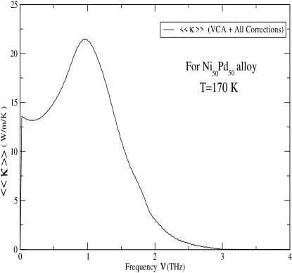
Figure 12: Thermal conductivity as a function of frequency for Ni₅₀Pd₅₀ alloys at T=170 K

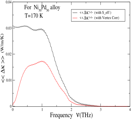
Figure 13: (Color Online) Corrections arising due to the disorder renormalization of the current term and the ladder approximation to the vertex correction

Direct comparison with the experimental data on these systems is difficult, because the experimental thermal conductivity also has a component arising out of the contribution from electrons. Figure 14 shows the temperature dependence of lattice conductivity. The top panel shows our theoretical result for the $Ni_{99}Pd_{01}$ alloy at three different frequencies. The bottom panel shows the experimental data expt1 on the total ( electronic + lattice ) thermal conductivity of the same 99-01 NiPd alloy. Since the frequency is not mentioned in the experimental data, we assume that it must be for low frequencies. The best comparison then will be between the middle (black) curve on the top panel and that in the bottom one. The two agree qualitatively, except at low temperatures where we expect the electronic contribution to dominate. In order to understand whether the deviation does arise from the electronic contribution, we have compared the top panel with the thermal conductivity of amorphous-Si feldmanetal , shown in the middle panel. In a-Si the electrons near the Fermi level are localized and hence cannot carry any current. Almost the entire contribution should come from the phonons. The behaviour of the two panels are quite similar.

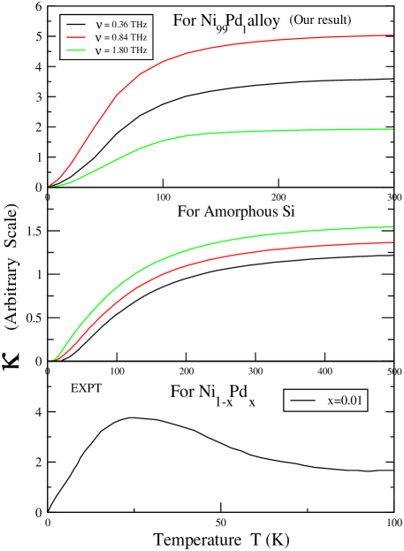
Figure 14: (Color Online) Thermal conductivity vs temperature T(K) for NiPd alloys and Amorphous Si. The top panel shows our results on the lattice conductivity for Ni₉₉Pd₀₁ alloy at three different frequency cut-off $\nu$. The middle panel shows the lattice conductivity for amorphous Si feldmanetal at three different cut-off frequency, while the panel at the bottom shows the experimental data expt1 for the total thermal conductivity (= lattice + electronic contribution) of the same Ni₉₉Pd₀₁ alloy.

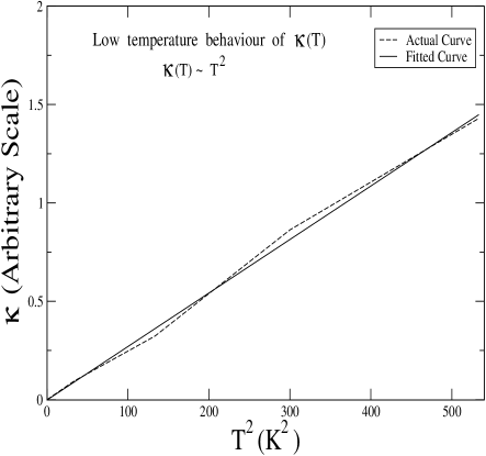
Figure 15: $\kappa$ vs $T^{2}$ for low temperatures for 50-50 NiPd alloy

A careful inspection of our results (top panel of Fig. 14) indicates that at low temperatures where only low-energy vibrations are excited, $\kappa(T)$ is approximately a quadratic function of $T$. Figure 15 shows a plot of $\kappa$ vs $T^{2}$. The calculated curve fits reasonably well with a straight line. This has been seen in experimental observations expt1 . Additional scattering processes leading to a different temperature dependence of lattice conductivity become apparent at higher temperatures. At $T>$25 K, $\kappa(T)$ rises smoothly to a $T$-independent saturated value. The dominant mechanism in this regime is the intrinsic harmonic diffusion of higher energy delocalized vibrations. These modes have not been well described by most previous theories.

The middle panel for amorphous Si has the similar qualitative behaviour for $\kappa(T)$ as ours. The three curves in this panel stands for three different frequencies. It is clear from the two panels (top and middle) that the saturation of $\kappa(T)$ for NiPd alloy starts at an earlier temperature as compared to that for amorphous Si. The magnitude of lattice conductivity in NiPd alloy is also larger than the value in amorphous Si, which is obvious because NiPd alloy is a metallic system with larger heat conduction.

In the bottom panel, which shows the experimental data for total thermal conductivity $\kappa=\kappa_{e}+\kappa_{g}$, where $\kappa_{e}$ is the electronic contribution and $\kappa_{g}$ the lattice contribution to the thermal conductivity, one can notice various similarities with the results of top panel. For example both the panels have (i) an approximate $T^{2}$-dependence expt1 in the low temperature regime and (ii) the value of $\kappa(T)$ approaching a T-independent final or saturated value at higher temperature side. In spite of these similarities, the overall agreement between the top and bottom panels is not satisfactory. This is mainly due to the existence of a broad peak like behaviour in the experimental curve unlike the theoretical results. This feature has been described in detail for a series of dilute alloys like Ni-Co, Ni-Fe and Ni-Cu in expt1 . We would like to ascribe this difference between the theoretical and experimental data to the extra electronic contribution to thermal conductivity hidden in the experimental curve.

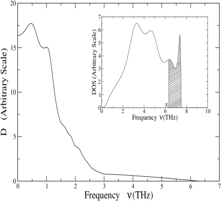
Figure 16: The configuration averaged thermal diffusivity $D(\nu)$ vs frequency $\nu$ for Ni₅₀Pd₅₀ alloy. The inside panel shows the phonon density of states for the same alloy.

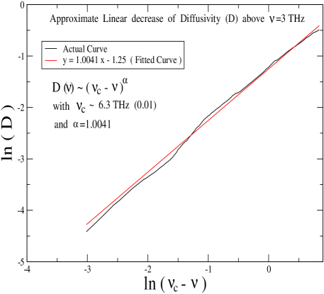
Figure 17: (Color Online) The behaviour of thermal diffusivity as a function of $(\nu_{c}-\nu)^{\alpha}$

The thermal diffusivities D($\nu$) are important because the effect of disorder is often manifested in them more directly than in the conductivities. Not only that the thermal diffusivity also give an approximate idea about the location of mobility edge as well as the fraction of delocalized states. Figure 16 shows the frequency dependence of diffusivity for Ni₅₀Pd₅₀ alloy. There are basically two regions of large thermal diffusivity, one near the lower frequency region ($\simeq 0.5THz$) and the other around a somewhat higher frequency region ($\simeq 1.25THz$). Above 3 THz, there is a smooth decrease of diffusivity approximately linear in frequency. The Fig 17 shows a plot of D($\nu$)$\propto(\nu_{c}-\nu)^{\alpha}$. At the critical frequency $\nu_{c}$= 6.3$\pm$ 0.014, $D(\nu)$ vanishes to within a very small level of noise. The critical exponent $\alpha\simeq 1.0041$. A knowledge of these critical parameters leads to the information about the location of mobility edge. The critical exponent of $\alpha\simeq 1$ in our case agrees with scaling and other theories of Anderson localization anderson and the critical frequency $\nu_{c}$ locates the mobility edge above which the diffusivity is zero in the infinite size limit. Once the mobility edge is located, the fraction of de-localized states may be obtained by evaluating the area under the $D(\nu)$ vs $\nu$ curve from $\nu=0$ to $\nu=\nu_{c}$. For Ni₅₀Pd₅₀ alloy ( see Fig. 16 ), the mobility edge is located at $\nu_{c}\simeq 6.314THz$. The panel at the top right corner of Fig. 16 shows the phonon density of states for the same alloy. The shaded region in this panel gives the information about the localized states. The fraction of localized states is actually the area beyond the critical frequency $\nu_{c}$.

VI Conclusions

We have formulated a theory for lattice thermal conductivity based on a realistic model. The augmented space approach allows us to go beyond the standard single-site mean-field theories and the augmented space recursion allows us to include, in the calculation of our averaged propagators, effects of joint fluctuations at more than one site. The augmented space approach has earlier been generalized to include effects of short-ranged ordering sro1 ; sro2 as well as local lattice relaxations due to large size mismatch of the constituents mis . Calculations including these effects have been earlier carried out for the electronic case. We propose to apply the same technique to phonons in disordered alloys. The scattering diagram approach proves to be useful in analyzing and calculating the disorder corrections to the averaged current. These are shown to be the dominant corrections and are related to the self-energy. Next in importance, we have studied the effect of vertex corrections arising out of the correlated propagation. We have shown explicitly how to obtain these corrections within the ladder diagram approximation. Our formalism explicitly takes into account fluctuations in masses, force constants and heat currents between different nuclei. For the calculation of the averaged propagators themselves we have used the augmented space recursion with the Beer-Pettifor terminator scheme. Our efficient Brillouin zone integration codes for disordered alloys makes the numerical calculation stable and accurate. We have already shown in an earlier communication am2 that the approximation involving termination of the matrix continued fraction expansion of the green matrix retains the essential herglotz analytic properties of the diagonal green function. Our numerical results on the temperature dependence of lattice conductivity favours a general trend of other theoretical results as well as the experimental data.

VII Acknowledgments

One of the authors (A.A.) would like to thank the Council of Scientific and Industrial Research, Govt. of India, for a fellowship during the time when this work was carried out.

References

• (1) A. Mookerjee, J. Phys. C: Solid State Phys. 6, L205 (1973).
• (2) R.J. Elliot, J.A. Krumhansl, and P.L. Leath, Rev. Mod. Phys. 46, 465 (1974).
• (3) W.A. Kamitakahara and B.N. Brockhouse, Phys. Rev. B 10, 1200 (1974).
• (4) A.A. Maradudin, Solid State Physics Vol. 18, edited by F. Seitz and D. Turnbull (Academic, New York, 1966).
• (5) P.G. Klemes, Proc. R. Soc. A 208, 108 (1951) ; Phys. Rev. 119, 507 (1960).
• (6) M.J. Ziman, Can. J. Phys. 34, 1256 (1956).
• (7) J. Callaway, Phys. Rev. 113, 1046 (1959).
• (8) J.E. Parrot, J. Phys. C: Solid State Phys. 2, 147 (1969).
• (9) J.K. Flicker and P.L. Leath, Phys. Rev. B 7, 2296(1973).
• (10) Y. Tsunoda, N. Kunitomi, N. Wakabayashi, R.M. Nicklow, and H.G. Smith, Phys. Rev. B 19, 2876 (1979).
• (11) S. Ghosh, P.L. Leath, and Morrel H. Cohen, Phys. Rev. B 66, 214206 (2002).
• (12) A.Alam and A. Mookerjee, Phys. Rev. B 69, 024205 (2004).
• (13) P.B. Allen and J.L. Feldman, Phys. Rev. B 48, 12 581 (1993).
• (14) P.L. Leath, Phys. Rev. B 2, 3078 (1970).
• (15) A.Alam and A. Mookerjee, Phys. Rev. B 71, 094210 (2005).
• (16) K.K. Saha and A. Mookerjee, Phys. Rev. B 70, 134205 (2004).
• (17) R.J. Hardy, Phys. Rev. 132, 168 (1963).
• (18) A. Mookerjee, J. Phys. C: Solid State Phys. 8, 1524 (1975).
• (19) A. Mookerjee, in Electronic Structure of Alloys, Surfaces and Clusters, edited by A. Mookerjee and D.D. Sarma. (Taylor and Francis, London, 2003).
• (20) A. Mookerjee, J. Phys. C: Solid State Phys. 9, 1225 (1976).
• (21) S.F. Edwards, Philos. Mag. 3, 1020 (1958).
• (22) J.S. Langer, Phys. Rev. 120, 714 (1960) ; J. Math. Phys. 2, 584 (1961).
• (23) S. Ghosh, N. Das, and A. Mookerjee, Int. J. Mod. Phys. B 21, 723 (1999).
• (24) P. L. Leath, Phys. Rev. 171, 725 (1968).
• (25) P.N. Aiyer, R.J. Elliott, J.A. Krummhansl and P.L. Leath, Phys. Rev. 181, 1006(1969).
• (26) B.G. Nickel and J.A. Krummhansl, Phys. Rev. B 4, 4354 (1971).
• (27) K.K. Saha, A. Mookerjee and O. Jepsen, Phys. Rev. B 71, 094207 (2005)
• (28) J.L. Feldman, M.D. Kluge, P.B. Allen, and F. Wooten, Phys. Rev. B 48, 12 589 (1993).
• (29) T. Farrell and D. Greig, J. Phys. C : Solid State Phys. 2, 1465 (1969).
• (30) P.A. Lee and T.V. Ramakrishnan, Rev. Mod. Phys. 57, 287 (1985)
• (31) A. Mookerjee and R. Prasad, Phys. Rev. B 48, 17724 (1993).
• (32) T. Saha, I. Dasgupta and A. Mookerjee, Phys. Rev. B 50,13267 (1994).
• (33) T. Saha and A. Mookerjee, J. Phys. Condens. Matter 8, 2915 (1996).