Phase Fluctuations in Strongly Coupled $d$-wave Superconductors

Abstract

We present a numerically exact solution for the BCS Hamiltonian at any temperature, including the degrees of freedom associated with classical phase, as well as amplitude, fluctuations via a Monte Carlo (MC) integration. This allows for an investigation over the whole range of couplings: from weak attraction, as in the well-known BCS limit, to the mainly unexplored strong-coupling regime of pronounced phase fluctuations. In the latter, for the first time two characteristic temperatures $T^{\star}$ and $T_{c}$, associated with short- and long-range ordering, respectively, can easily be identified in a mean-field-motivated Hamiltonian. $T^{\star}$ at the same time corresponds to the opening of a gap in the excitation spectrum. Besides introducing a novel procedure to study strongly coupled $d$-wave superconductors, our results indicate that classical phase fluctuations are not sufficient to explain the pseudo-gap features of high-temperature superconductors (HTS).

One of the most fascinating aspects of the HTS is that a theoretical description in traditional BCS terms – using Cooper pairs – is feasible, yet in many other aspects these materials seem to deviate considerably from the standard BCS behavior. Most notorious in this respect is the curious “pseudogap” (PG) phase in the underdoped regime. The PG has attracted enormous interest in recent years and its effects have been studied using a wide variety of techniques Corson_1 ,Lit_PG . It is identified as a dip in the density of states $N$$(\omega)$ below a temperature $T^{\star}$, which is higher than the superconducting (SC) critical temperature $T_{c}$, and its presence is sometimes attributed to a strong coupling between the charge carriers and accompanying phase fluctuations Emery_1 . If this is the case, then conventional mean-field (MF) methods should not work in describing the cuprates, since they cannot distinguish between $T^{\star}$ and $T_{c}$. For this reason, more elaborate techniques such as diagrammatic resummations or Quantum MC approximations have been used to address the many puzzling questions of strongly coupled superconductors. While for the case of superconductivity with $s$-wave symmetry (sSC) this effort can be carried out with the attractive Hubbard model Keller_1 , the direct study of phase fluctuations for $d$-wave superconductors (dSC) remains a challenge. To our knowledge, in the vast literature on cuprates there is no available model where the physics of a strongly coupled dSC with short coherence lengths and large phase fluctuations can be studied accurately, with nearly exact solutions Nazarenko . From the theory perspective, this is a conspicuous bottleneck in the HTS arena.

Here, we introduce a novel and simple approach to alleviate this problem. The proposed method allows for an unbiased treatment of phenomena associated with classical (thermal) phase fluctuations and non-coherent pair-binding. It represents an extension of the original solution of the pairing Hamiltonian and has been made possible mostly due to the advance of computational resources in the past decade. The focus is on the more interesting and important case - at least as far as HTS are concerned - of a nearest-neighbor (n.n.) attraction, necessary for dSC. With regards to the cuprates, this approach is only meaningful to the extent that the relevant phase fluctuations are thermal rather than quantum mechanical and in fact it has been argued Emery_1 that phase fluctuations in cuprates may be assumed as predominantly classical, with quantum (dynamical) fluctuations Kwon_1 suppressed.

Our approach is built on the insight that Hamiltonians that are quadratic in fermionic operators can be efficiently studied with the help of Monte Carlo techniques, as has been demonstrated in particular for the “double-exchange” model Dagotto_1 . This is possible here because the original interacting model has been stripped of quantum fluctuations in the pairing approximation. The Hamiltonian $H_{\rm SC}$ describes an effective attraction between fermions on a 2D lattice and is given by

$$H_{\rm SC} = -t\sum_{{\bf i},\delta,\sigma}c^{\dagger}_{{\bf i}\sigma}c_{{\bf i}+\delta\sigma}+V\sum_{{\bf i},\delta}|\Delta^{\delta}_{\bf i}|^{2}-\mu\sum_{\bf i}n_{\bf i}$$ (1)

$$-V\sum_{{\bf i},\delta}(c^{\dagger}_{{\bf i}+\delta\uparrow}c^{\dagger}_{{\bf i}\downarrow}+c^{\dagger}_{{\bf i}\uparrow}c^{\dagger}_{{\bf i}+\delta\downarrow})\Delta^{\delta}_{\bf i}+{\mbox{H.c.}}$$

where $t$ - the energy unit - is the hopping amplitude for electrons $c_{{\bf i}\sigma}$ on n.n. sites. $\mu$, the chemical potential, controls the particle density $\langle$$n$$\rangle$=1/$N$$\sum_{\bf i}$$n_{\bf i}$, $\delta$=$\pm$${\bf x,y}$ denotes n.n. on an $N$=$L$$\times$$L$ lattice, and in the standard derivation $\Delta^{\delta}_{\bf i}$=$\langle c_{{\bf i}\downarrow}c_{{\bf i}+\delta\uparrow}\rangle$ ($\langle$…$\rangle$ signals thermal averaging). In the usual MF approach to Eq.(1) the gap function $\Delta^{\delta}_{\bf i}$ is assumed a real number, but here we retain the degrees of freedom associated with the phases and therefore write $\Delta^{\delta}_{\bf i}$=$|\Delta_{\bf i}|\exp(i\phi^{\delta}_{\bf i})$. The amplitudes are regarded as site variables, whereas the phases are treated as link variables. $V$($>$0), the n.n. attraction, is assumed to be constant throughout the lattice, but inhomogeneous generalizations can be implemented in a straightforward manner. To calculate observables one needs to determine the corresponding partition function $Z_{\rm SC}$ at temperature $T$=1/$\beta$,

$$Z_{\rm SC}=\prod_{{\bf i}=1}^{2N}\int_{0}^{\infty}d|\Delta_{\bf i}|Z_{\rm cl}\int_{0}^{2\pi}d\phi^{x}_{\bf i}d\phi^{y}_{\bf i}Z_{c}(\{|\Delta_{\bf i}|\},\{\phi^{x,y}_{\bf i}\}),$$ (2)

which is calculated via a canonical MC integration over both $|\Delta_{\bf i}|$ and the phases $\{\phi^{x,y}_{\bf i}\}$. The electronic partition function $Z_{\rm c}$=Tr $\{e^{-\beta H_{\rm SC}^{\prime}(|\Delta_{\bf i}|,\phi^{x,y}_{\bf i})}\}$ ($H_{\rm SC}^{\prime}$ being the purely fermionic part of (1)) is obtained after exactly diagonalizing $H_{\rm SC}^{\prime}$ for a given fixed set of $|\Delta_{\bf i}|$’s and $\{\phi^{x,y}_{\bf i}\}$ and finding the eigenvalues $E_{n}^{\prime}$; it is then calculated in a standard fashion as $Z_{c}$=$\prod_{n=1}^{2N}(1+\exp(-\beta E_{n}^{\prime}))$ foot_ek . The classical part of $Z_{\rm SC}$ is $Z_{\rm cl}$=$e^{(-4\beta V)(\sum_{{\bf i}}|\Delta_{\bf i}|^{2})}$. The most CPU-time consuming task is the diagonalization leading to the eigenvalues $E_{n}^{\prime}$ for a given set of classical fields, limiting the lattice size. The results presented here were obtained for lattices up to $N$=14$\times$14, and for temperatures as low as $T$=0.002$t$. Observables such as the spectral function $A({\bf k},\omega)$, $N(\omega)$=$\sum_{\bf k}$$A({\bf k},\omega)$ or the optical conductivity $\sigma$$(\omega$) can be calculated straightforwardly Dagotto_1 . Here, however, we focus on other quantities of particular interest, namely the phase correlation function $S$(${\bf l}$=($l_{x}$,$l_{y}$))=$\frac{1}{N}$$\sum_{\bf i}$$\langle e^{i\phi^{x}_{\bf i}}e^{-i\phi^{x}_{{\bf i}+{\bf l}}}\rangle$, the “mixed” correlation $F$(${\bf l}$)=$\frac{1}{N}$$\sum_{\bf i}$$\langle e^{i\phi^{x}_{\bf i}}e^{-i\phi^{y}_{{\bf i}+{\bf l}}}\rangle$, which is determined by the internal symmetry of the pairing electrons as shown below foot_2 , and the gap $\Delta_{\rm MC}$$\equiv$$\frac{1}{N}$$\sum_{\bf i}$$\langle$$|$$\Delta_{\bf i}$$|$$\rangle$.

Figure 1(a) shows $S$($i_{x}$,$i_{y}$), $F$(0,0) on a 12$\times$12 lattice, at $\langle$$n$$\rangle$=1 and $T$=0.01. The different regimes emerging as $V$ is increased can easily be identified: (i) a BCS phase extending up to $V$$\simeq$3, where the correlation between n.n. sites (${\bf i}$, ${\bf j}$=${\bf i}$+${\bf x}$) and (${\bf j}$=${\bf i}$+($L$/2,0)) is virtually identical, (ii) an intermediate region 3.5$\lesssim$$V$$\lesssim$6, and (iii) the strongly coupled regime $V$$\gtrsim$6, with $short$-$range$ (SR) $phase$ $correlations$ only, at least at the lowest temperatures of our simulations. For the BCS state, $F$(0)$\approx$-1, equivalent to $\langle$$\Delta^{x}_{\bf i}$$\rangle$$\simeq$-$\langle$$\Delta^{y}_{\bf i}$$\rangle$, clearly exposing the $d_{x^{2}-y^{2}}$-character caused by strong scattering for the Fermi surface (FS) points ($\pm$$\pi$,0), (0,$\pm$$\pi$). This regime is characterized by a unique global phase, with only thermal fluctuations (and finite size effects) responsible for the small deviations from a perfect dSC foot_a . This is revealed by the phase histograms, which feature two well-defined Gaussian curves centered around $\phi^{x}_{0}$ and $\phi^{y}_{0}$=$\phi^{x}_{0}$+$\pi$, respectively. On the other hand, the until now unexplored strong-coupling regime of Eq.(1) is characterized by $distributions$ with multiple peaks and no evident global phase foot_ps . Such complicated distributions appear irrespective of starting configurations and other details of the MC process. Below, we will work with $H_{\rm SC}$ as well as with a $d$-wave-projected (“d-p”) model where $\Delta^{y}_{\bf i}$$\equiv$-$\Delta^{x}_{\bf i}$ is enforced, a commonly used approximation for dSC.

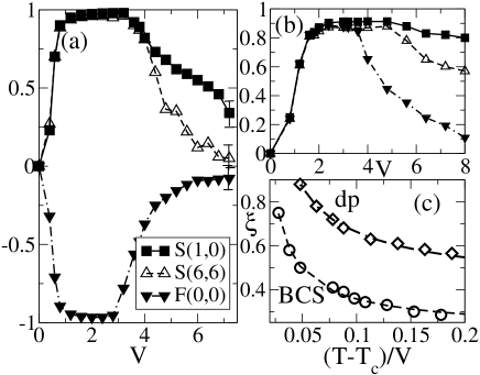
Figure 1: (a) The phase correlation functions $S$($V$), $F$($V$) at the shortest and maximum (linear) lattice distance at low $T$ and $\langle n\rangle$=1. (b) Same functions as in (a), now for $\langle n\rangle$$\sim$0.18, leading to (extended) $s$-wave behavior. The symbols stand for $S$(1,0) (filled squares), $S$(5,0) (open triangles) and $F$(0,0) (filled triangles). The statistical error is much smaller than the symbols for $V$$<$4, and roughly the symbol size for $V$$\lesssim$6. (c) The correlation length $\xi$($T$) for $V$=5.6 at $\langle$$n$$\rangle$=1 from the $H_{\rm SC}$ model. From the Kosterlitz-Thouless fit (broken line) we obtain $T_{c}$$\simeq$0.08. Also shown are results for the d-p model at $V$=4.8, that lead to $T_{c}$$\simeq$0.17.

To further explore the validity of the MC integration we have also performed calculations in the low-density limit, $\langle$$n$$\rangle$$\sim$0.18, with results for $S$(${\bf l}$), $F$(${\bf l}$) presented in Fig.1(b). Here, $F$(0,0)$\approx$1 emerges naturally ($T$ small), and therefore the expected $d_{x^{2}+y^{2}}$-symmetry ($\equiv$$s^{\star}$, $\cos{k_{x}}$+$\cos{k_{y}}$) is realized. Again, it is possible to differentiate between weak- and strong-coupling regimes, based on the same arguments as in (a).

$\Delta_{\rm MC}$($T$=0.01,$\langle$$n$$\rangle$=1) is shown in the table below for both $H_{\rm SC}$ and the d-p model ($\equiv$$\Delta_{\rm MC,dp}$). For small $V$, $\Delta_{\rm MC}$ barely deviates from its MF (dSC) value $\Delta_{\rm MF}$, but it is decidedly larger than $\Delta_{\rm MF}$ in the strongly fluctuating regime comment_gap . This, together with the results shown in Fig.1(a), where $F$(0,0) is very different from -1, signals the gradual transition from a dSC into what should be a $s^{\star}$+$i$$d$-SC Micnas_1 . The SC properties for large $V$ are not so much dictated by the FS topology (and band-filling) any more; instead the interaction $V$ forces all electronic states to take part in the pairing and not just the “preferred” ones near the FS, driving the system away from the $d$-wave state. Such a transition, believed to appear for any non-sSC, can easily be overlooked in studies biased towards dSC.

Table 1: Comparison of $\Delta_{\rm MC}$ ($\Delta_{\rm MC,dp}$) with the MF gap function, for both $d$- and conventional $s$-wave.

V		$\Delta^{10\times 10}_{\rm MF}$			$\Delta^{10\times 10}_{\rm MF,s}$			$\Delta^{10\times 10}_{\rm MC,dp}$			$\Delta^{10\times 10}_{\rm MC}$
1.2		0.322			0.241			0.32$\pm$0.02			0.32$\pm$0.02
2.0		0.627			0.666			0.62$\pm$0.02			0.62$\pm$0.03
4.0		1.420			1.747			1.42$\pm$0.03			1.63$\pm$0.18
4.8		1.743			2.213			1.90$\pm$0.20			2.05$\pm$0.18
5.6		2.066			2.636			2.50$\pm$0.20			2.50$\pm$0.20

For $V$$\gg$1, $\Delta_{\rm MC}$ is slightly smaller than the MF gap for the simple s-wave state, $\Delta_{\rm MF,s}$; thus, in this regime both the $d$-and the $s^{\star}$-wave gap will have almost the same amplitude Kotliar_1 and it may resemble a disordered sSC. Because of its $s$-wave component, the resulting state has a nodeless FS, i.e. no gapless excitations, and thus is strinkingly different from the weak-coupling state.

The investigation of the temperature dependence of $S$(${\bf l}$) for both $H_{\rm SC}$ and the d-p model allows us to introduce for the first time in a BCS-like Hamiltonian two characteristic temperatures $T^{\star}$ and $T_{c}$ in the case of strong coupling, in contrast to the BCS regime, where this distinction does not exist. We associate $T^{\star}$ with the temperature where SR phase correlations develop (defined here as $S(1,0)$$\geq$0.1, but other cutoffs lead to quite similar qualitative conclusions). On the other hand, $T_{c}$ is commonly identified with the onset of long-range phase coherence (here we use the criterium $S(L/2,0)$$\geq$0.1). $T^{\star}$ and $T_{c}$ are essentially identical for $V$ not too large (Fig.2(a)), and they are only clearly different for $V$$\gtrsim$3, with $T^{\star}$ larger than $T_{c}$ by a factor of 3-4 for $V$$>$5 (Fig.2(a)) foot_lowden . Based on such MC results, a phase diagram, presenting $T_{c}$ and $T^{\star}$ as a function of the pairing attraction, is displayed in Figs.2(b), (c). Remarkably, the values of $T_{c}$ reach a maximum $T^{max}_{c}$$\simeq$ 0.2 for $V_{\rm max}$$\approx$3 (similar to other such reported values), whereas $T^{\star}$ increases steadily with $V$ commentUV . For the “rigid” projected model (Fig.2(c)), $T^{\max}_{c}$$\simeq$0.3 , accompanied by a more prominent regime of SR correlations. The regime of a $d$-wave PG (dPG) is indicated, and although it is sizeable for the d-p model, it is a rather small window for the more realistic $H_{\rm SC}$. For the latter model, the state with a large difference between $T^{\star}$ and $T_{c}$ (typical for HTS) is only found for values of $V$ that do not lead to a dSC at low $T$, nowadays widely accepted for HTS, owing to strong experimental evidence. For $\langle$$n$$\rangle$$<$1, the dPG should be even less prominent than shown in Fig.2(b). This disagreement between theory and experiment puts the thermal phase-fluctuation scenario for HTS into serious doubt. $T_{c}$ itself is a continous function (Fig.2(b),(c)), smoothly connecting the limits $V$$\rightarrow$0,$\infty$, as predicted in an early work Schmitt_Rink_1 . Although the existence of $T^{\rm max}_{c}$ has long been known, this is - to our knowledge - the first time it has been directly established in the framework of $H_{\rm SC}$, since self-consistent methods are tracking $T^{\star}$ rather than $T_{c}$ foot_Ts . Yet, as demonstrated in Fig.2, they work very well for $V$ not excessively large.

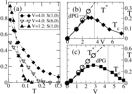
Figure 2: (a) SR and LR phase correlation functions vs. $T$ for two different values of $V$, covering the weak- and strong-coupling regime, for $\langle n\rangle$=1. Once $V$$\lesssim$2, no difference between short- and long-range correlations is observed, and $S$(6,0) ($V$=1.2) is not shown for reasons of clarity. Symbol sizes roughly match the errors. (b) The phase diagram for $H_{\rm SC}$ derived from (a); $T_{c}$ and $T^{\star}$ as explained in the text. (c) shows the phase diagram for the d-p model. Note the differences between (b) and (c). The $d$-wave PG regime (dPG) is indicated in both (b), (c). Beyond the dashed lines the $d$-wave character of $H_{\rm SC}$ is lost, whereas the d-p model incorporates higher harmonics as well.

For $V$$\gtrsim$$V_{\rm max}$ one presumably enters the realm of pronounced Kosterlitz-Thouless (KT) physics Kosterlitz_1 , whence $T_{c}$ is dictated by vortex binding rather than Cooper pairing. The critical temperature $T_{\rm KT}$$\equiv$$T_{c}$ in such models is proportional to 1/$V$, following a perturbative analysis, similar to what is found in Fig.2(b),(c). It is certainly non-trivial to establish whether or not KT-behavior is found for $H_{\rm SC}$, which, unlike the standard $X$$Y$ model, couples fermions to classical fields. For this purpose, we extract a correlation length $\xi$ by fitting $S$(${\bf l}$) with an exponential, $S$($r_{x}$)$\propto$$\exp(-r_{x}/\xi)$, and explore its temperature dependence, which should behave as $\xi$($T$)$\propto$$\exp$[A/$\sqrt{T-T_{c}}$]. In the case of $V$=5.6, such a KT analysis (for 0.10$\leq$$T$$\leq$0.35) produces a very good fit for $\xi$($T$) (see Fig.1(c)) and yields $T_{c}$=0.08$\pm$0.01, remarkably close to what has been established with our alternative definition of $T_{c}$ above. In addition, the exponential fit is not possible for $T$$\lesssim$0.08 - signalling that $H_{\rm SC}$ is entering a state with different scaling behavior. In a similar fashion, $T_{c}$ is found to be 0.17$(\pm$0.02) for the d-p model at $V$=4.8, only slightly lower than its estimate from $S$(${\bf l}$). Although the precise values cited above - having been obtained on relatively small lattices - need to be cautiously considered, our results are compatible with KT physics governing the region between $T_{c}$ and $T^{\star}$, even in the presence of fermions.

As the PG scenario would suggest, the effect of $T^{\star}$ is clearly visible in $N$($\omega$), which is shown for $V$=1.20 and $V$=4.0 in Fig.3. In the BCS limit (a), a gap appears for temperatures $T^{\star}$$\simeq$$T_{c}$=0.09 (compare to Fig.2(b)), whereas $N$($\omega$) shows non-correlated behavior and a van-Hove peak just above $T_{c}$. The remaining small peak at $\omega$=0 ($T$$<$$T_{c}$) is a finite size effect. At $V$=4.0 (Fig.3(b)), however, there is a wide region below $T^{\star}$$\simeq$0.30 (coinciding with the onset of SR fluctuations (Fig.2(b)) where a PG exists in $N$$(\omega)$ without LRO in the phase correlations.

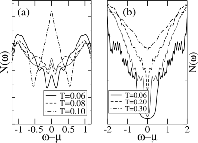
Figure 3: The $T$-dependent $N$($\omega$) (12$\times$12) for weak- ((a), $V$=1.2) and intermediate-coupling ((b), $V$=4) for $H_{\rm SC}$, illustrating the development of the PG as $T$ is lowered. In (a) the system is uncorrelated just above $T_{c}$, whereas in (b) the PG appears at $T^{\star}$ concurrently with SR ordering. For $T$=0.06, the deviation from the $d$-wave state becomes evident, and a gap $\omega_{0}$$\simeq$0.6 opens up. A broadening $\gamma$=0.05 was used. For reasons of comparison, the two thin lines represent the d-p model for T=0.15 ($V$=1.2), and T=0.20 ($V$=4), respectively.

As $T$ is lowered, spectral weight is continously removed from small energies, and the dip centered around $\omega$$\sim$0 deepens. $N$($\omega$) has a true gap at lower $T$ (finite spectral weight at $\omega$$\approx$0 stems from broadening only), reflecting the deviations from the $d_{x^{2}-y^{2}}$-symmetry noted before. In contrast, the projected model has a $d$-wave-like gap above $T_{c}$ (Fig.3(b)). Finite size effects in general influence subtle signals such as $d$-wave gaps considerably, but the observations above strongly validate our definition of $T^{\star}$ and demonstrate the influence of SRO on $N$($\omega$), which we have observed for all values of $V$.

We have also performed calculations for a model with diagonal hopping $t^{\prime}$=-1. For densities $\langle$$n$$\rangle$$\sim$0.2, this produces electron pockets around ($\pi$,0) (and related points) and, therefore, low-density dSC, confirmed in the same way as shown in Fig.1(a),(b). Our results can be summarized by stating that (a) the BCS region extends to very large $V$$\sim$12, (b) for $V$=10, it remains in the BCS state even as $\langle$$n$$\rangle$$\rightarrow$0, and (c) $T_{c}$ decreases concurrently, but so does $\Delta_{\rm MC}$, and, thus would $T^{\star}$, in disagreement with the well-established phase diagram. In addition, for intermediate $V$ and larger, $\mu$ is found to be below the band minimum. The resulting absence of nodes in $A$(${\bf k}$,$\omega$) is related to bound-pair formation, as previously noted Randeria_1 . Overall, it seems very difficult to reconcile our results here with the observed behavior of the cuprates.

Summarizing, a MC technique has been introduced for an unbiased investigation of the SC state as described in the ($d$-wave) pairing Hamiltonian. It reproduces both the BCS limit as well as the strong-coupling regime at all temperatures and densities. The establishment of a PG regime in the case of a strong pairing between two characteristic temperatures $T^{\star}$ and $T_{c}$ and an associated non-trivial phase diagram, has been numerically demonstrated. Our results for $H_{\rm SC}$ seem to indicate that the observed PG features of HTS cannot be reconciled with a (classical) phase-fluctuation-dominated dSC. The integration method presented here can easily be extended to study disordered systems as well as to simultaneously investigate the competition of several fluctuation channels, such as dSC, antiferromagnetism and charge order Alvarez_1 , in an unbiased fashion. As such, this method (maybe best dubbed “mean-field Monte Carlo”) should be an invaluable tool in unlocking the secrets of the cuprates and possibly other systems with strong-coupling aspects such as Bose-Einstein condensates in cold fermions.
Discussions with R. Zeyher, G. Khaliullin, P. Horsch, M. Randeria, R. Micnas and W. Metzner are gratefully acknowledged. E.D. is supported by grant NSF-DMR 0443144.

References

- [1] J. Corson et al., Nature (London) 398, 221 (1999).
- [2] A. Damascelli et al., Rev. Mod. Phys. 75, 473 (2003); Q. Chen et al., cond-mat/0404274.
- [3] V.J. Emery and S.A. Kivelson, Nature (London) 374, 434 (1995); Phys. Rev. Lett. 74, 3253 (1995).
- [4] R. Scalettar et al., Phys. Rev. Lett. 62, 1407 (1989); M. Randeria et al., Phys. Rev. Lett. 69, 2001 (1992); M. Keller et al., Phys. Rev. Lett. 86, 4612 (2001).
- [5] In A. Nazarenko et al., Phys. Rev. B 54, R768 (1996) it was shown that the -- model (0,0) has PS at large , rendering it unsuitable for the study of strongly coupled dSC.
- [6] H.-J. Kwon et al., Phys. Rev. Lett. 86, 3875 (2001).
- [7] E. Dagotto et al., Phys. Rep. 344, 1 (2001).
- [8] For a homogeneous system without phase fluctuations, the MF gap equations correspond to the saddle-point approximation of (2).
- [9] If only the phases are of interest, may be assumed constant (using, e.g., instead) and the integration performed over only.
- [10] A. Paramekanti et al., Phys. Rev. B 62, 6786 (2000).
- [11] MF suggests that for (=1) dSC competes with phase separation (PS). In snapshots of the charge distribution we have not observed any indications of PS. One might have to explicitely allow pairing in the particle-hole channel to study this issue in depth; in principle, this could be done by extending the framework used here.
- [12] The curious transition region is characterized by slow MC thermalization and convergence for .
- [13] R. Micnas et al., J. Phys. Cond. Matter 14, 9631 (2002). This is also confirmed by an analysis of the respective energies as well as by snapshots that show .
- [14] G. Kotliar, Phys. Rev. B 37, 3664 (1989).
- [15] This works in the low--limit, too. We find, e.g. =0.08 (=4, 0.2), so is smaller in this limit, as expected.
- [16] A similar phase diagram (with smaller ’s) can be found also in the t-U-V model (=1) for intermediate values of U, where both AF and SC coexist.
- [17] P. Nozieres and S. Schmitt-Rink, J. Low Temp. Phys. 59, 195 (1985).
- [18] () never drops to zero, unlike in MF calculations. Rather, at temperature and higher, is dominated by thermal (statistical) effects, leading to a spurious increase in .
- [19] J.M. Kosterlitz and D.J. Thouless, J. Phys. C 6, 1181 (1973).
- [20] M. Randeria et al., Phys. Rev. B 41, 327 (1990).
- [21] G. Alvarez et al., Phys. Rev. B 71, 014514 (2005).