Quasi-uniform in plane magnetization state of thin cylindrical dots in a square array and related anisotropy.

Abstract

The energy (magnetostatic, exchange and Zeeman terms) of a square array of cylindrical sub-micron dots made of soft ferromagnetic material is calculated analytically and minimized, taking into account quasi-uniformity of dots magnetization. The dependence of the equilibrium energy of the array on the direction of the externally applied magnetic field in the array plane is recovered, exhibiting the four-fold anisotropy. The anisotropy constant is calculated. Its values for different array geometries are in excellent agreement to the recent independent experiments. New eight-fold anisotropy effect is predicted. Theory involves no adjustable parameters.

Advances in fabrication of sub-micron ferromagnetic elements and their arrays produced a wealth of experiments, many of which are still waiting to be explained by theory. In particular, the first measurement of the four-fold anisotropy of the spin-wave frequencies in square arrays of circular permalloy dots was reported in 1997.Matthieu et al. (1997)

Discovery of the four-fold anisotropy of properties of a square lattice might seem obvious at first. However, a deeper look reveals that, while the distribution of stray fields in a square array of circular magnetic dots depends on orientation of their uniform magnetization in the array plane,Metlov (2000) the magnetostatic energy of the array is completely isotropic for any in-plane magnetization direction.Guslienko (1999) It directly follows from Maxwell equations that interaction of parallel dipoles (which a uniform magnetization state is) depends only on second powers of direction cosines and can only produce biaxial anisotropy (uniaxial in the array plane), even if the array is rectangular. But, as soon as both periods of the rectangular array are equal, the (in-plane) anisotropy of the magnetic energy of the uniformly magnetized array vanishes.

Thus, it is clear that the effect must come from some kind of non-uniform magnetization distribution within the dots. For example, the two-domain dots (divided by the oppositely-magnetized domains in half) do show the four-fold anisotropy.Guslienko (2001) It can be doubted, however, that such a configuration would survive the high (almost saturating) external field of magnetic resonance experiments.

Based on the approximate analytical approach to micromagnetics of thin flat sub-micron soft ferromagnetic elements,Metlov (2001) the ansatz for quasi-uniform magnetization distribution in a circular dot was proposed recently.Metlov and Guslienko (2004) Using this distribution as a starting point, the equilibrium (in the Ritz sense) energy of the square array of the dots in such a state is calculated below, comparing its angular dependence to the experiment.

The magnetization distributionMetlov (2001) can be expressed in terms of the complex function of complex variable:

$$w(z,\overline{z})=e^{\imath\varphi_{0}}\sqrt{\frac{p^{2}-e^{-2\imath\varphi_{0}}z^{2}}{p^{2}-e^{2\imath\varphi_{0}}\overline{z}^{2}}},$$ (1)

where $z=X/R+\imath Y/R$, $X$, $Y$ are Cartesian coordinates on the dot’s face, $R$ is the dot radius, $\imath=\sqrt{-1}$, line over a variable denotes the complex conjugation. Components of magnetization unit vector $\vec{m}$ are expressed through $w(z,\overline{z})$ as $m_{X}+\imath m_{Y}=2w/(1+w\overline{w})$ and $m_{Z}=(1-w\overline{w})/(1+w\overline{w})=0$. The dimensionless parameter $p>1$ describes displacement of skyrmions from the cylinder’s side, their centers (zeros of $w(z,\overline{z})$) are located at $X=\pm pR$, $Y=0$. The value of $p$ is to be found from minimization of the total energy of the array. For $p\rightarrow\infty$ the magnetization distribution is uniform, for finite $p$ the corresponding “leaf” quasi-uniform magnetization state is shown in Fig. 1.

Figure 1: The quasi-uniform magnetization distribution (1) with $p=2$. Lines inside the particle (its contour is outlined by the circle) are tangential to the magnetization vectors.

Compared to the original ansatz in Ref. Metlov and Guslienko, 2004 the expression (1) allows the average magnetization of the dot to point in arbitrary direction at an angle $\varphi_{0}$ w.r.t one of the array axis (this was unnecessary complication for a single dotMetlov and Guslienko (2004)).

To evaluate the magnetostatic energy of the array of such dots the magnetic charges formalism is used. It is based on the assumption that the problem is static and there are no currents in the system. This allows to express the stray magnetic field through a scalar potential, created by a system of “fictious” (introduced for mathematical convenience) magnetic charges. The volume density of these charges is $\sigma_{V}=-\mathrm{div}(\vec{m})$. On the boundary of magnetic material $\sigma_{V}$ reduces to the surface charge with the density $\sigma_{S}=(\vec{m}\cdot\vec{n})$ proportional to the (boundary) normal component of the magnetization vector. Both densities are normalized here by the saturation magnetization of the dot’s material ($M_{s}$). Inside of a dot with magnetization distribution (1) they are:

$$\sigma_{V} = \frac{2r\cos(\varphi-\varphi_{0})}{\sqrt{r^{4}+p^{4}-2p^{2}r^{2}\cos 2(\varphi-\varphi_{0})}},$$ (2)

$$\sigma_{S} = \frac{(p^{2}-1)\cos(\varphi-\varphi_{0})}{\sqrt{1+p^{4}-2p^{2}\cos 2(\varphi-\varphi_{0})}},$$ (3)

where $r\leq 1$ and $0<\varphi\leq 2\pi$ are the polar coordinates on the dot’s circular face, normalized by the dot radius. These are the rotated charge densities of Ref. Metlov and Guslienko, 2004.

To fully take into account periodicity of the array and all the implied interactions between dots, the density of magnetic charges is represented by its Fourier components:

$$\!\!\!\!\widetilde{A}_{n,m}(k_{z})\!\! = \!\!\frac{\rho\,\widetilde{a}_{n,m}}{T}\!\!\!\!\!\!\!\int\limits_{-L_{Z}/2}^{L_{Z}/2}\!\!\!\!\!\!\!e^{-2\pi\imath k_{Z}Z}\!\,{\mathrm{d}}Z\!=\!\frac{\widetilde{a}_{n,m}\rho\lambda\sin k_{Z}\!L_{Z}\!\pi}{k_{Z}L_{Z}\pi}$$ (4)

$$\!\!\!\!\widetilde{a}_{n,m}\!\! = \!\!\int\limits_{0}^{2\pi}\,{\mathrm{d}}\varphi\left(\sigma_{S}\,F|_{r=1}+\int\limits_{0}^{1}r\,{\mathrm{d}}r\,\sigma_{V}\,F\right),$$ (5)

$$\!\!\!\!F\!\! = \!\!e^{-2\pi\imath\rho(nX+mY)}=e^{-2\pi\imath\rho r(n\cos\varphi+m\sin\varphi)},$$ (6)

where $\rho=R/T$, $\lambda=L_{Z}/T$, $T>2R$ and $L_{Z}$ are the array period and thickness, $\widetilde{a}_{0,0}\equiv 0$ by construction.

Because the Fourier basis functions $F$ are also the eigenfunctions of the Laplace differential operator, the Poisson equation (resulting from the Maxwell equations under assumptions of the magnetic charges formalism) for the scalar potential becomes algebraic for its Fourier harmonics and can be readily solved. Normalized magnetostatic energy per array cell volume due to the interaction of the stray field with the magnetic charges $e_{M}=E_{M}/(\mu_{0}\gamma_{B}M_{S}^{2}T^{2}L_{Z})$ is then

$$e_{M}\!=\!\frac{\rho^{2}\lambda^{2}}{8\pi^{2}}\!\!\!\sum\limits_{n=-\infty}^{\infty}\sum\limits_{m=-\infty}^{\infty}\int\limits_{-\infty}^{\infty}\!\!\!\,{\mathrm{d}}\xi\frac{|\widetilde{a}_{n,m}|^{2}}{\lambda^{2}(n^{2}\!+\!m^{2})\!+\!\xi^{2}}\frac{\sin^{2}\xi\pi}{(\xi\pi)^{2}},$$ (7)

where $|\widetilde{a}_{n,m}|^{2}=\widetilde{a}_{n,m}\widetilde{a}_{-n,-m}$, $\xi=k_{Z}L_{Z}$, $\mu_{0}$ is permeability of vacuum in SI units, $\gamma_{B}$ is a units-dependent factorAharoni (1996) equal to $1$ in SI (in CGS $\mu_{0}=1$, $\gamma_{B}=4\pi$). The integral can be taken, allowing to represent

$$e_{M} = \frac{\rho^{2}}{8\pi^{2}}\!\!\!\sum\limits_{n=-\infty}^{\infty}\sum\limits_{m=-\infty}^{\infty}\!\!\!\!\!\frac{|\widetilde{a}_{n,m}|^{2}\mathrm{f}(2\pi\lambda\sqrt{n^{2}\!+\!m^{2}})}{n^{2}\!+\!m^{2}},$$ (8)

$$\mathrm{f}(x) = 1+\frac{e^{-x}-1}{x}.$$ (9)

To evaluate the 2-d Fourier components (5) let us first note that the denominator of both surface and volume charges can be expanded into the power series in $1/p^{2}$ (a small parameter in case the magnetization state in the dot is quasi-uniform) using the identity for the generating function of the Legendre polynomials $P_{i}(x)$

$$\frac{1}{\sqrt{r^{4}+p^{4}-2p^{2}r^{2}\cos\psi}}=\frac{1}{p^{2}}\sum\limits_{i=0}^{\infty}\frac{r^{2i}P_{i}(\cos\psi)}{p^{2i}}$$ (10)

where $\psi=2(\varphi\!-\!\varphi_{0})$. Using the identities for the generating functions of Bessel’s functions (formulas 6.521 in Ref. Gradshtejn and Ryzhik, 1963), the Fourier basis (6) can be represented as

$$F\!\!=\!\!\sum\limits_{k=-\infty}^{\infty}\sum\limits_{l=-\infty}^{\infty}\!(-\imath)^{k}(-1)^{l}J_{k}(\alpha\,n)J_{l}(\alpha\,m)e^{\imath(k+l)\varphi},$$ (11)

where $\alpha=2\pi\imath\rho r$ and $J_{k}(x)$ are the Bessel’s functions of the first kind.

In such a representation it is easy to evaluate the angular integral (5), which, for a given $i$, is non-zero only for $k+l=\pm(2j+1)$ with $j=1,2,\ldots,i$. This allows to remove (by making it finite) one infinite summation from a triple $i$, $k$, $l$ sum, resulting from expansions (10), (11). Then, using Bessel’s summation theorem, each of the remaining infinite sums over $k+l=(2j+1)$ and $k+l=-(2j+1)$ can be evaluated and combined, yielding the representation of $\widetilde{a}_{n,m}$ term for a given $i$ in terms of finite sum of Bessel’s functions of the orders $2j+1$ for $j=1,2,3,\ldots,i$. The resulting terms can be easily integrated in $r$ for the part of the integral (5), representing the volume charges. This calculation is quite voluminous in general.pac Fortunately, to obtain the expansion of the magnetostatic energy up to the $1/p^{4}$ (the first neglected term is $~{}\sim 1/p^{6}$) it is sufficient to evaluate the volume charges Fourier components for $i=0,1$ and the surface charges for $i=0,1,2$ (because of $p^{2}$ in Eq. 3).

The final result for the magnetostatic energy can be represented as

$$\!\!\!\!e_{M}\!\! = \!\!e_{0}\!+\!\frac{e_{1}\!+\!\cos(4\varphi_{0})e_{1a}}{p^{2}}\!+\!\frac{e_{2}\!+\!\cos(4\varphi_{0})e_{2a}}{p^{4}}\!+\!\ldots,$$ (12)

$$\!\!\!\!e_{i}\!\! = \!\!\rho^{2}\!\!\sum\limits_{m=0}^{\infty}\sum\limits_{n=1}^{\infty}\!\frac{K_{i}(\rho k_{m,n},\psi_{m,n})}{m^{2}+n^{2}}f(\lambda k_{m,n}),$$ (13)

where $k_{m,n}=2\pi\sqrt{m^{2}+n^{2}}$, $\psi_{m,n}=\frac{1}{2}\arctan(\frac{2mn}{n^{2}-m^{2}})$,

$$K_{0}(x) = J_{1}^{2}(x),$$ (14)

$$K_{1}(x) = J_{1}(x)J_{3}(x),$$ (15)

$$K_{1a}(x,\psi) = J_{1}(x)J_{3}(x)\cos(4\psi),$$ (16)

$$K_{2}(x) = -2J_{0}(x)J_{3}(x)/x,$$ (17)

$$K_{2a}(x,\psi) = (J_{3}(x)^{2}+2J_{1}(x)J_{5}(x))\cos(4\psi)/2.$$ (18)

Functions $e_{i}=e_{i}(\rho,\lambda)$ depend only on geometry of the problem and take into account the self-energy of the volume and surface charges, as well as interaction between them, both in a single dot and across all the dots in the array.

These expressions can be verified by renormalizing them to the unit of magnetic dot volume (as opposed to the volume of lattice cell) and taking the limit $T\rightarrow\infty$. In this case $e_{1a}=e_{2a}=0$, and $e_{0}$, $e_{1}$ and $e_{2}$ become identical to the corresponding functions $e^{\parallel}$, $e_{2}$ and $e_{4}$ of Ref. Metlov and Guslienko, 2004. Because the same thoroughly verified automaticpac procedure was used in deriving all the functions $K_{i}$, including the angular ones (marked with “a”), it can be expected with a high degree of confidence that all the expressions for $e_{i}(\rho,\lambda)$ are correct.

Looking at (12) it is immediately seen that for uniformly magnetized dots (when $p\rightarrow\infty$) the magnetostatic energy shows no angular dependence. The function $e_{0}$ is, thus, the energy of a square lattice of uniformly magnetized dots, which can be independently verified.

Compared to the above, evaluation of the exchange and Zeeman energy terms is trivial. Both contain no interaction between dots and can be evaluated for each dot separately. Actually, both were already calculated in Ref. Metlov and Guslienko, 2004. Renormalizing (2) from Ref. Metlov and Guslienko, 2004 as $e_{E}=E_{E}/(\mu_{0}\gamma_{B}M_{S}^{2}T^{2}L_{Z})$ and using the expression for the average magnetization (16) therein we get up to $1/p^{4}$:

$$e_{E}\!+\!e_{Z}\!=\!\frac{\pi}{\gamma_{B}\tau^{2}p^{4}}\!-\!\pi\rho^{2}h\cos(\varphi_{0}\!-\!\varphi_{1})\left(\!\!1-\frac{1}{12p^{4}}\!\!\right)\!+\!O\left(\!\frac{1}{p^{8}}\!\!\right)$$ (19)

where $\tau=T/L_{E}$, $L_{E}=\sqrt{C/(\mu_{0}M_{S}^{2})}$ is the exchange length of dot’s material, $h=H/(\mu_{0}\gamma_{B}M_{S})$ is the normalized field magnitude, and $\varphi_{1}$ is the angle of the in-plane applied field with respect to the lattice.

Now it remains to minimize the sum of (12) and (19) to find the equilibrium values of $p$ and $\varphi_{0}$. This results in two solutions for $\varphi_{0}$ separated by a small angle from the direction of the applied field $\varphi_{1}$, meaning that there will be hysteresis, depending on whether the current direction of the applied field was approached from bigger or smaller angles. Because the typical magnetic resonance measurement is performed in high sub-saturating magnetic field, this hysteresis can be expected to be small. Let us neglect it here for simplicity by putting $\varphi_{0}=\varphi_{1}$. Minimizing we get

$$p^{2}=\frac{h\pi\rho^{2}+12(\pi/(\gamma_{B}\tau^{2})+e_{2}+e_{2a}\cos 4\varphi_{1})}{6(-e_{1}-e_{1a}\cos 4\varphi_{1})}.$$ (20)

Let us assume for now that the denominator here is always positive (that is $e_{1}<0$, $e_{1a}>0$ and $|e_{1a}|<|e_{1}|$), which is the case for all the experiments analyzed below. Breaking of this assumption will be discussed at the end. The value of $p$ completely defines magnetic structure of dots in the array. Substituting it back, the equilibrium energy can also be expressed straightforwardly, but let us now concentrate on its angular dependence.

The largest (besides the constant term) Fourier harmonic in the angular dependence of the equilibrium energy is proportional to $\cos 4\varphi_{1}$, which can be clearly classified as the four-fold anisotropy. The higher harmonics, while modifying slightly the dependence itself, do not alter positions of extrema on the angular dependence with minimums located at $\varphi_{1}=\pi/4$, $3\pi/4$, $5\pi/4$, $7\pi/4$ and maximums at $\varphi_{1}=0$, $\pi/2$, $\pi$, and $3\pi/2$. Let us, thus, introduce the fourfold anisotropy constant, representing the equilibrium energy of a single dot (that is, normalized by the dot volume, which is the volume of magnetic material in the array cell) as $E=E_{0}+K_{4}\cos 4\varphi_{1}$ with $K_{4}>0$. The value of $K_{4}$ is the half of the equilibrium total energy (renormalized by the dot volume) difference between configurations at $\varphi_{1}=0$ and $\varphi_{1}=\pi/4$. Further, noting that in the resonance experiments the high external field plays a more notable role in stabilization of the “leaf” state than the exchange interaction (stabilizing it in the absence of the applied field), a limit of $\tau\rightarrow\infty$ is taken to simplify the expression into

$$K_{4}\!=\!\frac{\mu_{0}\gamma_{B}M_{s}^{2}}{2\pi\rho^{2}}\!\!\left(\!\!\frac{3(e_{1}\!-\!e_{1a})^{2}}{12(e_{2}\!-\!e_{2a})\!+\!\pi h\rho^{2}}\!-\!\frac{3(e_{1}\!+\!e_{1a})^{2}}{12(e_{2}\!+\!e_{2a})\!+\!\pi h\rho^{2}}\!\!\right)$$ (21)

The full expression, more accurate for the case of the array period comparable to the exchange length, can be easily obtained by the reader (it is also plotted in figures here). Nevertheless, for the subsequent comparison to experiments the precision of (21) is sufficient. At large applied fields $H/(\mu_{0}\gamma_{B}M_{S})\gg 1$ it is possible to expand $K_{4}$ asymptotically as

$$K_{4}=-\mu_{0}\gamma_{B}M_{S}^{2}\frac{6e_{1}e_{1a}}{\pi^{2}\rho^{4}h}+O\left(\frac{1}{h^{2}}\right).$$ (22)

Let us now apply the obtained knowledge to describe experiments found in literature. The first and foremost is the experiment found in Ref. Matthieu et al., 1997. To interpret it, the authors added the anisotropy of the form $K_{4}^{*}\sin^{2}\psi\cos^{2}\psi$ ($\psi$ is the angle between the magnetic moment in the dot and the lattice axis) into their numerical program for finding the resonance frequencies and fitted the angular dependence of the spectra to determine the $K_{4}^{*}$. Because the magnetization of the dot is close to uniform ($\psi=\varphi_{1}$) this term produces the shift in the total dot’s energy, followed by the measured spin-wave mode. Due to $\sin^{2}\varphi_{1}\cos^{2}\varphi_{1}$ oscillating between $0$ and $1/4$, while $\cos 4\varphi_{1}$ between $-1$ and $1$ with maximums of one corresponding to minimums of another (and vice versa), there is additional factor $-8$ linking the anisotropy in Ref. Matthieu et al., 1997 to the definition here. Another peculiarity is that the value of $K_{4}^{*}$ in Ref. Matthieu et al., 1997 tends to a constant value at large applied fields. This can not be explained by any model of the quasi-uniform state of infinite array, which at $h\rightarrow\infty$ must transform into the uniform state, showing no anisotropy. Thus, it seems another factor (probably due to the array shape effect) is present in the experiment. Assuming this factor is field-independent, let us simply add it, expressing $K_{4}^{*}=-8K_{4}-0.6\cdot 10^{5}\mathrm{erg}/\mathrm{cm}^{3}$, plotted in Fig. 2

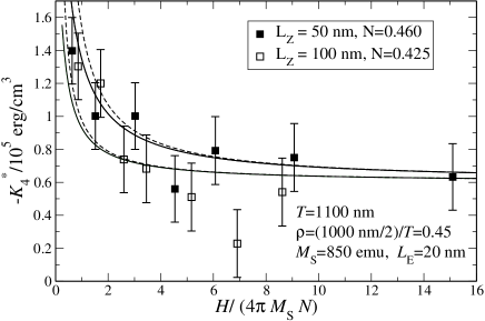
Figure 2: Dependence of the four-fold anisotropy constant $K_{4}^{*}$ on the magnitude of the in-plane magnetic field. Points are from Ref. Matthieu et al., 1997. The solid lines (21) and the full expression (without taking $\tau\rightarrow\infty$ limit) are indistinguishable. Dashed lines are from Eq. 22. The upper set of lines corresponds to $L_{Z}=100\mathrm{nm}$, the other to $L_{Z}=50\mathrm{nm}$. The values of the in-plane demagnetizing factor $N$ are shown in the legend.

(taking $M_{s}=850$ emu, typical for permalloy, but not specified in Ref. Matthieu et al., 1997) along with the experimental data. The agreement seems to be rather good, noting that the precision of the experiment did not allowMatthieu et al. (1997) to reliably resolve between dependencies of the $K_{4}^{*}$ for two considered arrays.

A much more precise recent experiment was done using FMR technique.Kakazei et al. (2006) In FMR it is impossible to change the value of the applied field, which was fixed at $1100\mathrm{Oe}$, but the authors tracked the anisotropy field as a function of the array geometry, measuring different arrays with periods from $1100$ to $2500$ nm. The anisotropy field can be expressed through the anisotropy constant as $H_{4}=2K_{4}/M_{S}$, which is plotted in Fig. 3

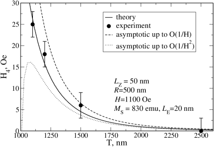
Figure 3: Dependence of the four-fold anisotropy field $H_{4}$ on the inter-dot spacing. Points are from Ref. Kakazei et al., 2006. The solid line plots the Eq. 21 (again, the finite $\tau$ case is indistinguishable). Dashed and dotted lines show the asymptotes of (21) up to $O(1/h)$ (Eq. 22) and $O(1/h^{2})$ respectively. The value of $L_{E}$ obtained from the measuredKakazei et al. (2004) exchange constant ($A=C/2$).

along with the array parameters and the experimental data from Ref. Kakazei et al., 2006. The agreement is excellent for the case of $K_{4}$ calculated from (21), whereas the simplified asymptotic expression (22) and its higher order equivalent are clearly not good enough at such a small field.

Let us now look back at (20). It turns out that it is quite possible for the denominator to become zero and negative. This happens for dot geometries approximately defined by the numerical fit $R_{cr}/T=0.51-0.37\cdot(L_{z}/T)+0.13\cdot(L_{z}/T)^{2}$ in $0<L_{z}/T<1$ with fixing the resulting $R_{cr}/T$ to 0.5 when it exceeds this value. At radii above $R_{cr}$ the parameter $p$ becomes imaginary for some directions of the applied field, which corresponds to the transition to the so-called “flower” state. In this state (as opposed to initially considered “leaf”) the magnetization vectors diverge outwards of the line through the dot center parallel to the applied field. All the expressions here still apply in the case of “flower” (with imaginary $p$), but, because of the additional “flower”$\leftrightarrow$“leaf” transition the dots array with the $R>R_{cr}$ shows the additional eight-fold (!) anisotropy of the form $K_{4}\cos 4\varphi_{1}+K_{8}\cos 8\varphi_{1}$ with $K_{4}$ still given by (21) and $K_{8}<0$. This transition and the resulting anisotropy will be explored in the forthcoming extended paper on the subject.

To conclude, the considered problem belongs to the class, where the leading order energy contribution vanishes due to symmetry, and the system is governed by higher order energy terms. In most other cases details of the quasi-uniform magnetization distribution make only small (and often negligible) corrections to the leading order results, but here they are responsible for the completely new effect, absent in the leading order. Apart from quantitatively describing the four-fold anisotropy in the magnetic dot arrays, the presented theory asks for experiments on thicker dots, which should reveal the new eight-fold anisotropy effect. This theory can be expected to describe it quantitatively.

Support by the internal project K1010104 is appreciated. I would like to thank Vladimir Kambersky for valuable remarks, especially for doubting the initial conjecture that $-e_{1}\pm e_{1a}>0$, which pushed me for a recheck and the discovery of the “flower” state in the system.

References

- Matthieu et al. (1997) C. Matthieu, C. Hartmann, M. Bauer, O. Buettner, S. Riedling, B. Roos, S. O. Demokritov, B. Hillebrands, B. Bartenian, C. Chappert, et al., Appl. Phys. Lett. 70, 2912 (1997).
- Metlov (2000) K. L. Metlov, J. Magn. Magn. Mat. 215–216, 37 (2000).
- Guslienko (1999) K. Y. Guslienko, Appl. Phys. Lett. 75, 394 (1999).
- Guslienko (2001) K. Y. Guslienko, Phys. Lett. A 278, 293 (2001).
- Metlov (2001) K. L. Metlov (2001), arXiv:cond-mat/0102311.
- Metlov and Guslienko (2004) K. L. Metlov and K. Y. Guslienko, Phys. Rev. B 70, 052406 (2004).
- Aharoni (1996) A. Aharoni, Introduction to the theory of ferromagnetism (Oxford University Press, Oxford, 1996).
- Gradshtejn and Ryzhik (1963) I. S. Gradshtejn and I. M. Ryzhik, Tables of series, products, and integrals (Gos. izdatelstvo fiz.-mat. literatury, Moskva, 1963), note that formulas 6.521.3 and 6.521.4 in both 1953 and 1963 editions of this book contain errors.
- (9) I have written a Mathematica package to do it for a given , which I can share upon request.
- Kakazei et al. (2006) G. N. Kakazei, M. D. Costa, Y. G. Pogorelov, V. O. Golub, V. Novosad, T. Okuno, P. E. Wigen, and P. C. Hammel, Phys. Rev. B (2006), accepted for publication.
- Kakazei et al. (2004) G. N. Kakazei, P. E. Wigen, K. Y. Guslienko, V. Novosad, A. Slavin, V. Golub, N. Lesnik, and Y. Otani, Appl. Phys. Lett. 85, 443 (2004).