Constraints on the two-particle distribution function due to the permutational symmetry of the higher order distribution functions

Abstract

We investigate how the range of parameters that specify the two-particle distribution function is restricted if we require that this function be obtained from the $n^{\rm th}$ order distribution functions that are symmetric with respect to the permutation of any two particles. We consider the simple case when each variable in the distribution functions can take only two values. Results for all $n$ values are given, including the limit of $n\to\infty$. We use our results to obtain bounds on the allowed values of magnetization and magnetic susceptibility in an $n$ particle Fermi fluid.

I Introduction

Two particle coordinate distribution function is one of the central objects of statistical mechanics Balescu (1975); Reichl (1998). Any such distribution must satisfy the following requirements. Firstly, it must be non-negative everywhere. Secondly, it must be normalized. Thirdly, for systems of $n$ indistinguishable particles, it is obtained by integrating out (or summing out) $n-2$ coordinates of the $n$ particle distribution function that is invariant under the permutation of any of its particles. While the first two requirements give explicit constrains on the possible forms of two particle distribution functions, this is not the case for the third requirement. Clearly, it follows from the third requirement that the two particle distribution must be symmetric with respect to the permutation of the two particles. However, the third requirement is more restrictive, i.e. not all symmetric non-negative and normalized two particle distribution functions can be obtained from symmetric $n$ particle distribution functions. Therefore, it is of interest to understand what are the explicit constraints on the possible forms the two particle distribution function (other than its symmetry) that follow from the third requirement. This knowledge can be useful in various ways. For example, in the case of equilibrium distributions it would give us an opportunity to tell which features of the two particle distribution function are due to the permutational symmetry of the Hamiltonian and which ones are due to its explicit form. In particular, as will be shown in a specific example below, symmetry imposed bounds on the values of certain physical quantities can be obtained. Another field of applications includes solving various correlation function integral equations Hansen and McDonald (1986); Kalikmanov (2001) by iterational procedures . For such equations initial guess function that incorporate the symmetry information can provide faster convergence.

Our goal in this paper is two-fold. Firstly, we would like to work out a simple example that shows explicitly how the two particle distribution function is restricted by the fact that it is obtained from the permutationally symmetric $n$ particle distribution function. Secondly, we want to apply this result to a physical system and show that it leads to certain bounds on the allowed values of the physical properties for this system.

II Obtaining constraints on the two-particle distribution function

Consider the $n$ variable joint probability distribution function $f_{n}(x_{1},x_{2},...,x_{n})$ in which each variable can take only two values, $-1$ and $1$. The function $f_{n}(x_{1},x_{2},...,x_{n})$ is assumed to be symmetric with respect to the permutation of its variables, non-negative everywhere and normalized. We will use the normalization in which $f_{n}$ is normalized to one. Such distributions can describe quite different physical situations. For example, as discussed in more detail below, after suitable rescaling $f_{n}$ can be the joint probability distribution of the $z$ spin components of $n$ particles in a Fermi fluid. It can also describe outcomes of a coin-tossing experiment involving $n$ identical coins, or its analogues. Since we will be dealing with reducing higher order functions to lower order ones it is useful to introduce parametrizations of such joint probability distributions that will have simple relations for the functions of different orders. For our purposes a convenient set of parameters is given by the expansion coefficients of $f_{n}(x_{1},x_{2},...,x_{n})$ in terms of products of functions $\phi_{0}(x_{i})$ and $\phi_{1}(x_{i})$, that are defined as follows, $\phi_{0}(x_{i})=1$ and $\phi_{1}(x_{i})=x_{i}$. The expansion of a normalized $f_{n}(x_{1},x_{2},...,x_{n})$ has the following form Naya et al. (1964)

$$f_{n}(x_{1},x_{2},...,x_{n})=\frac{1}{2^{n}}\left(1+\sum_{i=1}^{n}\langle x_{i}\rangle x_{i}+\!\sum_{j>i=1}^{n}\langle x_{i}x_{j}\rangle x_{i}x_{j}+\!\!\!\!\sum_{k>j>i=1}^{n}\langle x_{i}x_{j}x_{k}\rangle x_{i}x_{j}x_{k}+...+\langle x_{1}x_{2}...x_{n}\rangle x_{1}x_{2}...x_{n}\right),$$ (1)

where the expansion coefficients are the moments of $f_{n}(x_{1},x_{2},...,x_{n})$ of different orders. For $f_{n}(x_{1},x_{2},...,x_{n})$ with a given $n$, the series terminates at the term involving the $n^{\rm th}$ order moment. For the functions that are symmetric with respect to the permutation of any two of their variables, moments of the same order must be the same. Thus, the normalized and symmetric function $f_{n}(x_{1},x_{2},...,x_{n})$ is completely defined by $n$ parameters, $\langle x_{1}\rangle,\langle x_{1}x_{2}\rangle,...,\langle x_{1}x_{2}...x_{n}\rangle$. The allowed range of these parameters is obtained from the requirement that $f_{n}(x_{1},x_{2},...,x_{n})\geq 0$ for all coordinate values. Since there are $2^{n}$ such values this leads to $2^{n}$ inequalities. However, due to the symmetry of $f_{n}(x_{1},x_{2},...,x_{n})$ only $n+1$ of these inequalities are independent. As will be shown in the specific examples below, these inequalities specify a closed region of the allowed values in the $n$ dimensional space of parameters $\langle x_{1}\rangle,\langle x_{1}x_{2}\rangle,...,\langle x_{1}x_{2}...x_{n}\rangle$.

Let us consider the allowed range of parameters for the function $f_{2}(x_{1},x_{2})$ provided that it is normalized, symmetric and non-negative. The function $f_{2}(x_{1},x_{2})$ is completely specified by $\langle x_{1}\rangle$ and $\langle x_{1}x_{2}\rangle$. The requirement of the non-negativity leads to the following three inequalities

$$1+2\langle x_{1}\rangle+\langle x_{1}x_{2}\rangle \geq 0,$$

$$1-2\langle x_{1}\rangle+\langle x_{1}x_{2}\rangle \geq 0,$$

$$1-\langle x_{1}x_{2}\rangle \geq 0.$$ (2)

If these relations are treated as the equalities, then they define three nonparallel straight lines in the $\langle x_{1}\rangle,\langle x_{1}x_{2}\rangle$ plane. The inequalities define a region inside a triangle whose vertices are the intersection points of the three straight lines. The $\langle x_{1}\rangle,\langle x_{1}x_{2}\rangle$ coordinates for the vertices of the triangle are (-1, 1), (0, -1), (1, 1). The region of allowed values is shown on Fig. 1.

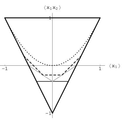
Figure 1: The regions of allowed values for the $f_{2}$ parameters $\langle x_{1}\rangle$ and $\langle x_{1}x_{2}\rangle$. The region inside the big isosceles triangle is allowed if $f_{2}$ is required to be non-negative, normalized, and permutationally symmetric. The areas of this triangle above different lines represent the allowed parameter regions if $f_{2}$ is obtained from a permutationally symmetric $f_{n}$. The horizontal solid line corresponds to $n=3$, the gray line to $n=4$, the dashed line to $n=5$, the dotted parabola to $n\to\infty$.

Now we would like to find out how this region is reduced by the additional requirement that the function $f_{2}(x_{1},x_{2})$ is obtained by summing out variable $x_{3}$ in the distribution function $f_{3}(x_{1},x_{2},x_{3})$ that is non-negativity, normalized to one, and symmetric with respect to the permutation of any of its three variables. Such function $f_{3}(x_{1},x_{2},x_{3})$ can be completely specified by parameters $\langle x_{1}\rangle$, $\langle x_{1}x_{2}\rangle$, and $\langle x_{1}x_{2}x_{3}\rangle$. The requirement of the non-negativity for $f_{3}(x_{1},x_{2},x_{3})$ leads to the following four inequalities

$$1+3\langle x_{1}\rangle+3\langle x_{1}x_{2}\rangle+\langle x_{1}x_{2}x_{3}\rangle \geq 0,$$

$$1-3\langle x_{1}\rangle+3\langle x_{1}x_{2}\rangle-\langle x_{1}x_{2}x_{3}\rangle \geq 0,$$

$$1+\langle x_{1}\rangle-\langle x_{1}x_{2}\rangle-\langle x_{1}x_{2}x_{3}\rangle \geq 0,$$

$$1-\langle x_{1}\rangle-\langle x_{1}x_{2}\rangle+\langle x_{1}x_{2}x_{3}\rangle \geq 0.$$ (3)

These four inequalities define a tetrahedral region in the $\langle x_{1}\rangle,\langle x_{1}x_{2}\rangle,\langle x_{1}x_{2}x_{3}\rangle$ space. The vertices of the tetrahedron have the following $\langle x_{1}\rangle,\langle x_{1}x_{2}\rangle,\langle x_{1}x_{2}x_{3}\rangle$ coordinates, (-1, 1, -1), ( -1/3, -1/3, 1), (1/3, -1/3, -1), (1, 1, 1).

If $f_{2}(x_{1},x_{2})$ is obtained from $f_{3}(x_{1},x_{2},x_{3})$ then the allowed range of its parameters $\langle x_{1}\rangle$ and $\langle x_{1}x_{2}\rangle$ must be the same that these parameters have in $f_{3}(x_{1},x_{2},x_{3})$. This latter range is given by the projection of the tetrahedral parameter region for $f_{3}(x_{1},x_{2},x_{3})$ onto the $\langle x_{1}\rangle,\langle x_{1}x_{2}\rangle$ plane. Since tetrahedron is a convex polytope the projection that we seek is either a convex tetragonal or triangular region. If we plot the actual values of the $\langle x_{1}\rangle,\langle x_{1}x_{2}\rangle$ coordinates of the vertices of the tetrahedron given above then the tetragonal region is obtained (Fig. 1). Thus, the requirement that $f_{2}(x_{1},x_{2})$ is obtained from the permutationally symmetric $f_{3}(x_{1},x_{2},x_{3})$ reduces the range of allowed values of $\langle x_{1}\rangle$ and $\langle x_{1}x_{2}\rangle$.

We can apply the same procedure to obtain the restrictions on the $f_{2}(x_{1},x_{2})$ parameters if it is obtained from any higher order symmetric $f_{n}(x_{1},x_{2},...,x_{n})$. The allowed range of $n$ parameters for $f_{n}(x_{1},x_{2},...,x_{n})$ is a region inside a simplex in $n$ dimensions Munkres (1993). The allowed range of values for $\langle x_{1}\rangle$ and $\langle x_{1}x_{2}\rangle$ is determined by projecting this region on the $\langle x_{1}\rangle,\langle x_{1}x_{2}\rangle$ plane. The projection is a convex $(n+1)$-gonal region. The $\langle x_{1}\rangle,\langle x_{1}x_{2}\rangle$ coordinates of the vertices of the $(n+1)$-gon are obtained from the coordinates of the simplex vertices. These latter coordinates are obtained from $n+1$ inequalities that specify the simplex region. Inspection of the results for several small $n$ values obtained by explicit calculations allows one to come up with the general formulas for the coordinates of the polygon vertices for arbitrary $n$,

$$\langle x_{1}\rangle=\frac{2i-n}{n},\qquad\langle x_{1}x_{2}\rangle=\frac{(2i-n)^{2}-n}{n(n-1)},$$ (4)

where $i$ is an integer taking the values from $0$ to $n$. Examples for $n=4$ and $n=5$ are given on Fig. 1.

The obtained results allow one to draw certain conclusions about possible changes of $f_{2}(x_{1},x_{2})$ in an $n$ particle system. Suppose that the $f_{2}(x_{1},x_{2})$ parameters lie in the region that is cut out by going to an $n+1$ particle system. Then adding an extra particle to the $n$ particle system will necessarily change $f_{2}(x_{1},x_{2})$. If, however, the $f_{2}(x_{1},x_{2})$ parameters lie in the region that is not affected by going to an $n+1$ particle system then $f_{2}(x_{1},x_{2})$ may or may not change depending on the details of the extra particle addition.

Eqs. (4) can be viewed as a parametric form of the function $\langle x_{1}x_{2}\rangle=\langle x_{1}x_{2}\rangle(\langle x_{1}\rangle)$. The explicit form of this function can be obtained by expressing $i$ through $\langle x_{1}\rangle$ from the first of Eqs. (4) and substituting it into the equation for $\langle x_{1}x_{2}\rangle$. This gives

$$\langle x_{1}x_{2}\rangle=\frac{n\langle x_{1}\rangle^{2}-1}{n-1}.$$ (5)

It can be deduced from this equation that for each $n$ the polygon that defines the region of the allowed values is inscribed in a parabola.

For large systems it is of interest to investigate the limit of $n\to\infty$. It is easy to check using Eqs. (4) that both $\langle x_{1}\rangle$ and $\langle x_{1}x_{2}\rangle$ change continuously in the limit $n\to\infty$. Taking this limit in Eq. (5) we obtain

$$\langle x_{1}x_{2}\rangle=\langle x_{1}\rangle^{2}.$$ (6)

The corresponding region of allowed values is shown on Fig.1. Thus, as $n\to\infty$, the broken lines formed by $n-2$ sides of each $n$-gone converge to the parabola given by Eq. (6).

To investigate how fast the areas $A_{n}$’s of the polygons converge to their limit at $n\to\infty$ we use the formula for the area of a polygon Beyer (1987) to obtain

$$A_{n}=\frac{4(n+1)}{3n},\qquad\frac{A_{n}-A_{\infty}}{A_{\infty}}=\frac{1}{n}.$$ (7)

From the statistical mechanics standpoint this means that if we want to approximate the $n\to\infty$ region by a finite $n$ region then we need to consider rather large values of $n$. For example, if we require a $1\%$ accuracy then $n\geq 100$ must be considered.

III Effect of constraints on the correlation function

It is customary in statistical mechanics to separate the two particle probability distribution into the uncorrelated and correlated parts as

$$f_{2}(x_{1},x_{2})=f_{1}(x_{1})f_{1}(x_{2})+g_{2}(x_{1},x_{2}),$$ (8)

where

$$f_{1}(x_{1})=\sum_{x_{2}=\pm 1}f_{2}(x_{1},x_{2})$$ (9)

is the one particle distribution function and the correlation function $g_{2}(x_{1},x_{2})$ is defined by Eq. (8). Let us consider how the above constraints on $f_{2}(x_{1},x_{2})$ affect $g_{2}(x_{1},x_{2})$ and $f_{1}(x_{1})$. The functions $f_{1}(x_{1})$ and $g(x_{1},x_{2})$ can be written in terms of parameters $\langle x_{1}\rangle$ and $\langle x_{1}x_{2}\rangle$ as

$$f_{1}(x_{1}) = \frac{1}{2}\left(1+\langle x_{1}\rangle x_{1}\right),$$ (10)

$$g_{2}(x_{1},x_{2}) = \frac{1}{4}\left(\langle x_{1}x_{2}\rangle-\langle x_{1}\rangle^{2}\right)x_{1}x_{2}.$$ (11)

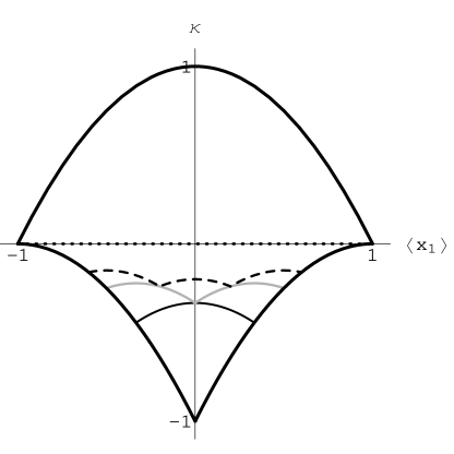
Figure 2: The regions of allowed values for $\langle x_{1}\rangle$ and the correlation parameter $\kappa$. The region inside the figure formed by the thick solid lines is allowed if $f_{2}$ is required to be non-negative, normalized, and permutationally symmetric. The areas of this figure above different lines represent the allowed parameter regions if $f_{2}$ is obtained from a permutationally symmetric $f_{n}$. The thin solid line corresponds to $n=3$, the gray line to $n=4$, the dashed line to $n=5$, the horizontal dotted line to $n\to\infty$.

The parameter $\langle x_{1}\rangle$ (that completely specifies $f_{1}(x_{1})$) can be viewed as the degree of inhomogeneity since $f_{1}(x_{1})$ is constant when $\langle x_{1}\rangle=0$. The parameter $\kappa=\langle x_{1}x_{2}\rangle-\langle x_{1}\rangle^{2}$ characterizes the strength of the correlations. A surprising result of this analysis is that the line of the zero correlations on the $\langle x_{1}\rangle,\langle x_{1}x_{2}\rangle$ plane is the same as the limiting parabola given by Eq. (6). To see more explicitly how the correlation function is affected by the constraints, we redraw Fig. 1 in the $\langle x_{1}\rangle$, $\kappa$ space, as shown on Fig. 2.

Fig. 2 shows some interesting relations between the correlations and inhomogeneity for finite $n$. For a fixed $\langle x_{1}\rangle$ the allowed range of $\kappa$ is always a single segment whereas for a fixed $\kappa$ the allowed range of $\langle x_{1}\rangle$ can be either a single segment or, for sufficiently negative $\kappa$ a few separate segments. For this latter case it is impossible to go from one segment to another without changing the correlations. Interestingly, the correlations with the largest negative $\kappa$ require $f_{1}(x_{1})$ to be homogeneous for even $n$ but inhomogeneous for odd $n$. For $n\to\infty$, only the correlations with $\kappa\geq 0$ are allowed. In this limit, the allowed correlation functions must have $g_{2}(1,1)\geq 0$, $g_{2}(-1,-1)\geq 0$, and $g_{2}(1,-1)\leq 0$, $g_{2}(1,-1)\leq 0$

As can be seen on Figs. 1, 2, the constraints from the higher order distribution functions do not affect the maximum possible range of $\langle x_{1}\rangle$. This is to be expected since $\langle x_{1}\rangle$ is the only parameter characterizing $f_{1}$ and for every physical $f_{1}$ we can construct a permutationally symmetric $f_{n}$ as a product of $n$ $f_{1}$’s.

IV Bounds on the magnetization and magnetic susceptibility in spin $1/2$ quantum fluids

As an example of application of our results to a physical system we will investigate allowed ranges of average $z$ component of the total spin $\langle S^{z}\rangle$ and its variance $\langle(S^{z})^{2}\rangle-\langle S^{z}\rangle^{2}$ in a Fermi fluid Huang (1987) or Bose fluid with (iso)spin $1/2$ Nikuni and Williams (2003). Here

$$S^{z}=\sum_{i}s^{z}_{i}=\frac{\hbar}{2}\sum_{i}\sigma^{z}_{i}$$ (12)

and $s^{z}_{i}$ is the $z$ component of spin for particle $i$ and $\sigma^{z}_{i}$ is the corresponding Pauli matrix. The quantities $\langle S^{z}\rangle$ and $\langle(S^{z})^{2}\rangle-\langle S^{z}\rangle^{2}$ are of interest because for a wide range of systems in equilibrium they are proportional to the magnetization and magnetic susceptibility, respectively. Note, however, that our results for $\langle S^{z}\rangle$ and $\langle(S^{z})^{2}\rangle-\langle S^{z}\rangle^{2}$ apply to arbitrary states, not necessarily equilibrium ones. Since $\sigma^{z}_{i}$ has the eigenvalues of $\pm 1$ we can see that function $f_{n}$ discussed above can be viewed as the probability distribution of the $\sigma^{z}_{i}$ eigenvalues for $n$ particles with variable $x_{i}$ denoting eigenvalues of $\sigma^{z}_{i}$.

Before proceeding with our analysis we need to be sure that the quantum nature of the Fermi or Bose fluid does not impose additional restrictions on $f_{n}$. This is indeed the case. We will not go into details of the proof here. The outline of the proof is as follows. It can be shown that the vertices of $n$ dimensional simplex domains for the allowed $f_{n}$ parameters correspond to the total density matrices composed of the wave functions that are eigenstates of $S^{z}$ with a given eigenvalue. (For an $n$ particle system there are $n+1$ different $S^{z}$ eigenvalues, as many as there are vertices.) Since the density matrices for the vertices exist and since any simplex domain is convex, the density matrices for the points inside the simplex also exist. Thus, $\sigma^{z}_{i}$’s can be rigorously treated as classical variables as far as the joint distributions of their eigenvalues are concerned.

Using Eq. (12) and replacing $\sigma^{z}_{i}$ with $x_{i}$ we obtain for the average $S^{z}$ and its variance.

$$\langle S^{z}\rangle = \frac{\hbar}{2}n\langle x_{1}\rangle$$

$$\langle(S^{z})^{2}\rangle-\langle S^{z}\rangle^{2} = \frac{\hbar^{2}}{4}\left(n(n-1)\langle x_{1}x_{2}\rangle-n^{2}\langle x_{1}\rangle^{2}+n\right)$$

Using the allowed range of parameters for $\langle x_{1}\rangle$ and $\langle x_{1}x_{2}\rangle$ we can obtain the allowed domains for $\langle S^{z}\rangle$ and $\langle(S^{z})^{2}\rangle-\langle S^{z}\rangle^{2}$. The results are shown on Fig. 3.

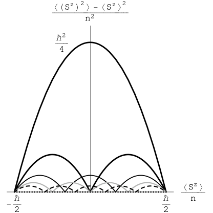
Figure 3: The regions of allowed values for $\langle S^{z}\rangle/n$ and $\left(\langle(S^{z})^{2}\rangle-\langle S^{z}\rangle^{2}\right)/n^{2}$. The regions bounded from above by the big parabolic arc and from below by series of $n$ smaller arcs drawn in different styles are allowed for the $n$ particle Fermi fluid. The thick solid line corresponds to $n=2$, the thin solid line to $n=3$, the gray line to $n=4$, the dashed line to $n=5$, the dotted straight line to $n\to\infty$.

Qualitative physical interpretation of these results is straightforward. Each point of the allowed domain with $\langle(S^{z})^{2}\rangle-\langle S^{z}\rangle^{2}=0$ correspond to the total density matrices composed of eigenstates of $S^{z}$ with the same eigenvalue, i. e. $\langle S^{z}\rangle$ is a multiple of $\hbar/2$. For $\langle S^{z}\rangle$ that is not a multiple of $\hbar/2$ $\langle(S^{z})^{2}\rangle-\langle S^{z}\rangle^{2}$ is necessarily greater than zero (because not all spins are either up or down). Generally, for smaller $\langle S^{z}\rangle$ values the allowed range of $\langle(S^{z})^{2}\rangle-\langle S^{z}\rangle^{2}$ is larger.

Consider a Fermi fluid whose Hamiltonian involves the coupling to the magnetic field ${\bf{\cal H}}$ of the form $H_{m}=-\frac{e}{mc}S^{z}{\cal H}$. For the system in the thermal equilibrium the magnetization per unit volume, $M$ is given by

$$M=\frac{e}{mcV}\langle S^{z}\rangle$$ (14)

If $H_{m}$ commutes with the total Hamiltonian then the magnetic susceptibility, $\chi$ is given by

$$\chi=\frac{\beta}{V}\left(\frac{e}{mc}\right)^{2}\left(\langle(S^{z})^{2}\rangle-\langle S^{z}\rangle^{2}\right)$$ (15)

Thus, with suitable rescaling, Fig. 3 describes the allowed domains of $M$ and $\chi$ for any model satisfying the above requirements. As can be expected, no such model can be diamagnetic ($\chi$ is always $\geq 0$).

V Concluding remarks

The generalization of our analysis to the functions whose variable can take more than two values is straightforward. If each variable of $f_{2}(x_{1},x_{2})$ is allowed to take $l$ values, then $f_{2}(x_{1},x_{2})$ can be completely specified by $(l(l+1)-2)/2$ parameters. Parameters of the higher order functions can always be chosen in such a way that they include $(l(l+1)-2)/2$ parameters of $f_{2}(x_{1},x_{2})$. Constraints on the latter parameters are obtained by projecting the allowed parameter range of the higher order function on the $f_{2}(x_{1},x_{2})$ parameter subspace.

The case of continuous coordinates is more complicated since infinitely many parameters are needed to specify the distribution functions. In this case, our approach can be used to investigate the finite dimensional subspaces of the $f_{2}(x_{1},x_{2})$ parameter space in some regions of interest, e. g., in the vicinity of functions with a certain characteristic wavelength.