Lennard–Jones and Lattice Models of Driven Fluids

Abstract

We introduce a nonequilibrium off–lattice model for anisotropic phenomena in fluids. This is a Lennard–Jones generalization of the driven lattice–gas model in which the particles’ spatial coordinates vary continuously. A comparison between the two models allows us to discuss some exceptional, hardly realistic features of the original discrete system —which has been considered a prototype for nonequilibrium anisotropic phase transitions. We thus help to clarify open issues, and discuss on the implications of our observations for future investigation of anisotropic phase transitions.

The concept of nonequilibrium phase transition (NPT) Haken ; gar ; Cross helps our present understanding of many complex phenomena including, for instance, the jamming in traffic flow on highways Traffic , the origin of life Ferreira , and the pre–humans transition to mammals Treves . Many studies of NPTs have focused on lattice systems Liggett ; Zia ; Privman ; Droz ; Marro ; Hinrichsen ; Odor . This is because lattice realizations are simpler than in continuum space, e.g., they sometimes allow for exact results and are easier to be implemented in a computer. Furthermore, a bunch of emerging techniques may now be applied to lattice systems, including nonequilibrium statistical field theory. A general amazing result from these studies is that lattice models often capture the essentials of social organisms, epidemics, glasses, electrical circuits, transport, hydrodynamics, colloids, networks, and markets, for example.

The driven lattice gas (DLG) KLS , a crude model of “super ionic currents”water , has become the theoreticians’ prototype for anisotropic NPTs. The DLG consists of a lattice gas with the particles hopping preferentially along one of the lattice directions, say $\hat{x}.$ One may imagine this is induced by an external drive, $E\hat{x},$ e.g., an applied electric field assuming the particles are positive ions. Consequently, for periodic boundary conditions, a particle current and an anisotropic interface set up along $\hat{x}$ at low temperature, $T<T_{E}.$ That is, a liquid–like phase which is striped then coexists with its gas. More specifically, assuming —for simplicity and concreteness— the square lattice half filled of particles, Monte Carlo (MC) simulations show that the function $T_{E}$ monotonically increases with $E$ from the Onsager value $T_{0}=T_{\text{Onsager}}=2.269Jk_{B}^{-1}$ to $T_{\infty}\simeq 1.4T_{\text{Onsager}}.$ This limit corresponds to a nonequilibrium critical point. As a matter of fact, it was numerically shown to belong to a universality class other than the Onsager one, e.g., MC data indicates $\beta\simeq 0.33$ (instead of the Ising value $\beta=1/8$ in two dimensions) for the order parameter critical exponent Marro ; beta4 ; beta5 ; beta6 .

Statistical field theory is a complementary approach to the understanding of nonequilibrium ordering in the DLG. The derivation of a general mesoscopic description is still an open issue, however. Two different approaches have been proposed. The driven diffusive system (DDS) Zia ; beta2 ; beta3 , which is a Langevin type of equation aimed at capturing all the relevant symmetries, predicts that the current will induce a predominant mean–field behavior and, in particular, $\beta=1/2.$ The anisotropic diffusive system (ADS) paco , which follows after a non–rigorous coarse graining of the master equation, rules out the relevance of the current and leads to the above–indicated MC critical exponent for $E\rightarrow\infty.$ However, the ADS approach reduces to the DDS for finite $E,$ a fact which is hard to be fitted to MC data, and both contain disquieting features problemas .

In any case, field theoretical studies have constantly demanded further numerical efforts, and the DLG is nowadays the most thoroughly studied system showing an anisotropic NPT. The topic is not exhausted, however. On the contrary, there remain unresolved matters such as the above mentioned issues concerning critical and mesoscopic behaviors, and the fact that $T_{E}$ increases with $E$, which is counterintuitive Zia2 . Another significative question concerns the observation of triangular anisotropies at early times after a rapid MC quench from the homogenous state to $T<T_{E}.$ The triangles happen to point against the field, which is contrary to the prediction from the DDS continuum equation triang1 .

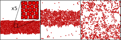
Figure 1: Typical configurations during the stationary regime of the DLJF subject to a horizontal field of intensity $E^{\ast}=1.$ These graphs, which are for $N=900$ particles and density $\rho^{\ast}=0.30,$ illustrate, from left to right, (i) coexistence of a solid and its vapor (the configuration shown is for temperature $T^{\ast}=0.20),$ (ii) liquid–vapor coexistence $(T^{\ast}=0.35),$ and (iii) a disordered, fluid phase $(T^{\ast}=0.50).$ The left–most graph shows a detail of the solid strip. The particles, which move in a square box of side $\sqrt{N/\rho^{\ast}}$, are given here an arbitrary size, namely, diameter$=1.1\sigma$.

This paper reports on a new effort towards better understanding basic features of NPTs. With this aim, we here present a description of driven systems with continuous variation of the particles’ spatial coordinates —instead of the discrete variations in the DLG. We hope this will provide a more realistic model for computer simulation of anisotropic fluids. Our strategy to set up the model is to follow as closely as possible the DLG. That is, we analyze an off–lattice representation of the DLG, namely, a microscopically continuum with the same symmetries and hopefully criticality. Investigating these questions happens to clarify the puzzling situation indicated above concerning the outstanding behavior of the DLG. The clue is that the DLG is, in a sense, pathological.

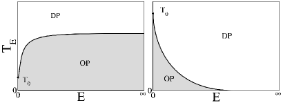
Figure 2: Schematic phase diagrams for the three models, as defined in the main text, showing ordered (OP) and disordered (DP) phases. The left graph is for the DLG, for which $T_{0}=T_{\text{Onsager}}.$ The graph on the right is valid for both the NDLG, i.e., the DLG with next–nearest–neighbor (NNN) hops, for which $T_{0}=2.35T_{\text{Onsager}},$ and the DLJF, for which $T_{0}^{\ast}=0.459$ smit .

Consider a fluid consisting of $N$ particles in a two–dimensional $L\times L$ box with periodic boundary conditions. Interactions are according to a truncated and shifted Lennard–Jones (LJ) potential Allen :

$$V(r_{ij})=\left\{\begin{array}[]{cl}V_{LJ}(r_{ij})-V_{LJ}(r_{c}),&\text{if }r_{ij}<r_{c}\\ 0,&\text{if }r_{ij}\geq r_{c}.\end{array}\right.$$

Here, $r_{ij}=\left|\vec{r_{i}}-\vec{r_{j}}\right|$ is the relative distance between particles $i$ and $j,$ $V_{LJ}(r)=4\epsilon\left[(\sigma/r)^{12}-(\sigma/r)^{6}\right],$ $\epsilon$ and $\sigma$ are our energy and length units, respectively, and $r_{c}$ is the cut-off that we shall fix at $r_{c}=2.5\sigma$. The preferential hopping will be implemented as in the lattice, i.e., by adding a drive to the potential energy. Consequently, the familiar energy balance is (assuming $k_{B}\equiv 1$ hereafter):

$$-T^{-1}\left[\left(H(\vec{c}^{\prime})-H(\vec{c})\right)+E\hat{x}\cdot\vec{\delta}\right].$$ (1)

Where $\vec{c}=\left\{\vec{r_{1}},...,\vec{r_{N}}\right\}$ stands for configurations, $H(\vec{c})=\sum_{i<j}V(r_{ij})$, and $\vec{\delta}=\vec{r_{i}}^{\prime}-\vec{r_{i}}$ is the attempted particle displacement. Defining the latter is a critical step because, as we shall show, the resulting (nonequilibrium) steady state will depend, even qualitatively on this choice. Lacking a lattice, the field is the only source of anisotropy, and any trial move should only be constrained by a maximum displacement in the radial direction. That is, we take $0<|\vec{\delta}|<\Delta,$ where $\Delta=0.5\sigma$ in the simulations reported here. The temperature $T$, number density $\rho=N/L^{2}$, and field variables will be reduced according to $T^{\ast}=T/\epsilon$, $\rho^{\ast}=\rho\sigma^{2}$, and $E^{\ast}=E\sigma/\epsilon$, respectively. Our model thus reduces for $E\rightarrow 0$ to the truncated and shifted LJ fluid, one of the most studied models in the computer simulation of fluids Allen ; smit .

We studied this driven LJ fluid (DLJF) in the computer by the MC method using a “canonical ensemble”, namely, fixed values for $N,$ $\rho^{\ast},$ $T^{\ast},$ and $E^{\ast}.$ Simulations involved up to $N=10^{4}$ particles with parameters ranging as follows: $0.5\leq E^{\ast}\leq 1.5,$ $0.20\leq\rho^{\ast}\leq 0.60,$ $0.15\leq T^{\ast}\leq 0.55.$ The typical configurations one observes are illustrated in Fig. 1. As its equilibrium counterpart, the DLJF exhibits three different phases (at least): vapor, liquid, and solid (sort of close–packing phase; see the left–most graph in Fig. 1). At intermediate densities and low enough $T^{\ast},$ vapor and a condensed phase segregate from each other. The condensed droplet (see Fig. 1) is not near circular as it generally occurs in equilibrium, but strip–like extending along the field direction. A detailed study of each of these phases will be reported elsewhere manolo ; we here focus on more general features.

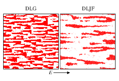
Figure 3: Triangular anisotropies as observed at early times for $E=1$ in computer simulations of the lattice (left) and the off–lattice (right) models defined in the main text. The DLG configuration is for $t=6\times 10^{4}$ MCS in a 128$\times$128 lattice with $N=7372$ particles and $T=0.4T_{\text{Onsager}}.$ The DLJF configuration is for $t=1.5\times 10^{5}$ MCS, $N=10^{4}$ particles, $\rho^{\ast}=0.20$ and $T^{\ast}=0.23.$

A main observation is that the DLJF closely resembles the DLG in that both depict a particle current and the corresponding anisotropic interface. However, they differ in an essential feature, as illustrated by Fig. 2. That is, contrary to the DLG, for which $T_{E}$ increases with $E,$ the DLJF shows a transition temperature $T_{E}$ which decreases with increasing $E.$ The latter behavior was expectable. In fact, as $E$ is increased, the effect of the potential energy in the balance Eq. (1) becomes weaker and, consequently, the cohesive forces between particles tend to become negligible. Therefore, unlike for the DLG, there is no phase transition for a large enough field, and $T_{E}\rightarrow 0$ for $E\rightarrow\infty$ in the DLJF. Confirming this, typical configurations in this case are fully homogeneous for any $T$ under a sufficiently large field $E.$ One may think of variations of the DLJF for which $T_{E\rightarrow\infty}=const>0,$ which is more realistic, but the present one follows more closely the DLG microscopic strategy based on Eq. (1) manolo .

Concerning the early process of kinetic ordering, one observes triangular anisotropies in the DLJF that point along the field direction. That is, the early–time anisotropies in the off–lattice case (right graph in Fig. 3) are similar to the ones predicted by the DDS, and so they point along the field, contrary to the ones observed in the discrete DLG (left graph in Fig. 3).

The above observations altogether suggest a unique exceptionality of the DLG behavior. This is to be associated with the fact that a driven particle is geometrically restrained in the DLG. In order to show this, we studied the lattice with an infinite drive extending the hopping to next–nearest–neighbors (see also Refs.triang2 ; szabo ). As illustrated in Fig. 4, this introduces further relevant directions in the lattice, so that the resulting model, to be named here NDLG, is expected to behave closer to the DLJF. This is confirmed. For example, one observes in the discrete NDLG that, as in the continuum DLJF, $T_{E}$ decreases with increasing $E$ —though from $T_{0}=2.35T_{\text{Onsager}}$ in this case. This is illustrated in Fig. 2.

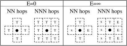
Figure 4: Schematic comparison of the accessible sites a particle (at the center, marked with a dot) has for nearest–neighbors (NN) and next–nearest–neighbors (NNN) hops at equilibrium (left) and in the presence of a large horizontal field (right). The particle–hole exchange between neighbors may be forbidden (x), depend only on the potential energy (T), or occur with probability 1 (E).

There is also interesting information in the two–point correlation function and its Fourier transform, $S(\vec{k}).$ In fact, the DLG displays (more clearly above criticality) slow decay of two–point correlations pedro due to the detailed balance violation for $E\neq 0.$ For a half–filled lattice, this function is $C(\vec{r})=\left\langle s_{\vec{q}}\,s_{\vec{r}+\vec{q}}\right\rangle-1/4,$ where $s_{\vec{q}}$ is the occupation number at site $\vec{q}$ and the steady average $\left\langle...\right\rangle$ involves also averaging over $\vec{q}.$ Analysis of the components along the field, $C(x,0),$ and transverse to it, $C(0,y),$ shows that correlations are qualitatively similar for the DLG and the NDLG —although somewhat weaker along the field for NNN hops. That is, allowing for a particle to surpass its forward neighbor does not modify correlations. The power–law behavior translates into a discontinuity of $S(\vec{k})$ pedro , namely, $\lim_{k_{x}\rightarrow 0}S(k_{x},0)\neq\lim_{k_{y}\rightarrow 0}S(0,k_{y}),$ which is clearly confirmed in Fig. 5 for both NN and NNN hops.

The above shows that the nature of correlations is not enough to determine the phase diagram. There are already indications of this from the study of equilibrium systems, and also from other nonequilibrium models. That is, one may have a qualitatively different phase diagram but essentially the same two–point correlations by modifying the microscopic dynamics manolo ; szabo . It follows, in particular, that the exceptional behavior of the DLG cannot be understood just by invoking the functions $C(\vec{r})$ and $S(\vec{k})$ or crude arguments concerning symmetries. The fact that particles are constrained to travel precisely along the two principal lattice directions in the DLG is the cause for its singular behavior. Allowing jumping along intermediate directions, as in both the NDLG and the DLJF, modifies essentially the phase diagram but not features —such as power–law correlations— that seem intrinsic of the nonequilibrium nature of the phenomenon.

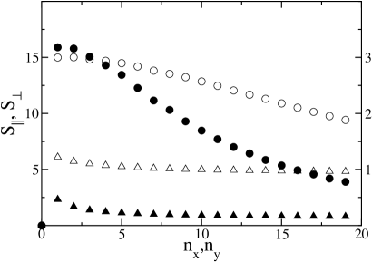
Figure 5: Parallel (circles) and transverse (triangles) components of the structure factor above criticality for the DLG on a $128\times 128$ lattice with NN interactions (filled symbols, left scale) at $T=1.58$ and NNN interactions (empty symbols, right scale) at $T=1.$ Temperatures normalized to $T_{\text{Onsager}}$. Here, $n_{x,y}=128k_{x,y}/2\pi$.

Rutenberg and Yeung triang2 also performed quenching experiments for variations of the DLG. They showed, in particular, that minor modifications in the DLG dynamics may lead to an inversion of the triangular anisotropies during the formation of clusters which finally condense into strips. Our observations above prove that such nonuniversal behavior goes beyond kinetics, namely, it also applies to the stationary state.

The unique exceptionality of the DLG has some important consequences. One is that this model involves features that are not frequent in nature. There are situations in which a drive induces stripes but not necessarily DLG behavior. The fact that a particle impedes the freedom of the one behind to move along $\hat{x}$ for a large enough field may only occur very seldom in cooperative transport. The NDLG is more realistic in this sense. In any case, the great effort devoted to the DLG during two decades has revealed important properties of both nonequilibrium steady states and anisotropic phase transitions, and there are some unresolved issues yet. For example, a general mesoscopic description which captures the exceptionality of the DLG remains elusive. According to our observations above, such a description needs to include the microscopic details of transverse dynamics which, in particular, should allow one to distinguish between the DLG and the NDLG. On the other hand, it ensues that, due to its uniqueness, the DLG does not have a simple off-lattice analog. This is because the ordering agent in the DLG is more the lattice geometry than the field itself. The fact that one needs to be very careful when modeling nonequilibrium phenomena —one may induce both a wrong critical behavior and an spurious phase diagram— ensues again in this example. This seems not to be so dramatic in equilibrium where, for example, the lattice gas is a useful oversimplification of a LJ fluid.

Finally, we remark that a novel fluid model in which the particles move in a continuum space has been introduced in this paper. The particle ‘infinite freedom’ is realistic, as it is also the LJ potential. It may contain some of the essential physics in a class of nonequilibrium anisotropic phenomena and phase transitions. On the other hand, the model is simple enough to be useful in computer simulations, and it is endowed of even–simpler and functional lattice analogs such as the NDLG.

We acknowledge very useful discussions with E. Albano, M. A. Muñoz, and F. de los Santos, and financial support from MEyC and FEDER (project FIS2005-00791).

References

- (1) H. Haken, Rev. Mod. Phys. 47, 67 (1975).
- (2) L. Garrido, Far from Equilibrium Phase Transitions, Sitges Conference 1988 (Springer Verlag, Berlin, Germany, 1989).
- (3) M.C. Cross and P.C. Hohenberg, Rev. Mod. Phys. 65, 851 (1993).
- (4) K. Nagel and M. Schreckenberg, J. Phys. I (France) 2, 2221 (1992); D. Chowdhury et al., Phys. Rep 329, 199 (2000).
- (5) C. P. Ferreira and J. F. Fontanari, Phys. Rev. E 65, 021902 (2002).
- (6) A. Treves and Y. Roudi, in Methods and Models in Neurophysics, Les Houches School 2003 (Elsevier, 2005).
- (7) T. M. Liggett, Interacting Particle Systems, (Springer Verlag, Heidelberg, Germany, 1985).
- (8) B. Schmittmann and R. K. P. Zia, in Statistical Mechanics of Driven Diffusive Systems in Phase Transitions and Critical Phenomena, Vol. 17, edited by C. Domb and J. L. Lebowitz (Academic, London, U.K., 1996).
- (9) V. Privman, Nonequilibrium Statistical Mechanics in One Dimension, (Cambridge University Press, Cambridge, U.K., 1996).
- (10) B. Chopard and M. Droz, Cellular Automata Modeling of Physical Systems, (Cambridge University Press, Cambridge, U.K., 1998).
- (11) J. Marro and R. Dickman, Nonequilibrium Phase Transitions in Lattice Models, (Cambridge University Press, Cambridge, U.K., 1999).
- (12) H. Hinrichsen, Adv. Phys. 49, 815 (2000).
- (13) G. Ódor, Rev. Mod. Phys. 76, 663 (2004).
- (14) S. Katz, J. L. Lebowitz, and H. Spohn, J. Stat. Phys. 34, 497 (1984).
- (15) A. F. Goncharov et al., Phys. Rev. Lett. 94, 125508 (2005).
- (16) A. Achahbar, P. L. Garrido, J. Marro, and M. A. Muñoz, Phys. Rev. Lett. 87, 195702 (2001).
- (17) E. V. Albano and G. Saracco, Phys. Rev. Lett. 88, 145701 (2002).
- (18) E. V. Albano and G. Saracco, Phys. Rev. Lett. 92, 029602 (2004).
- (19) K. Leung and J. L. Cardy, J. Stat. Phys. 44, 567 (1986).
- (20) H. K. Janssen and B. Schmittmann, Z. Phys. B 63, 517; ibid 64, 503 (1986).
- (21) F. de los Santos, P. L. Garrido, and M.A. Muñoz, Physica A 296, 364 (2001).
- (22) A. Achahbar et al., to be published.
- (23) B. Schmittmann and R. K. P. Zia, Phys. Rep. 301, 45 (1998).
- (24) F. J. Alexander, C. A. Laberge, J. L. Lebowitz, and R. K. P. Zia, J. Stat. Phys. 82, 1133 (1996).
- (25) M. P. Allen and D. J. Tidlesley, Computer Simulations of Liquids, (Oxford University Press, Oxford, U.K., 1987).
- (26) B. Smit and D. Frenkel, J. Chem. Phys. 94, 5663 (1991).
- (27) M. Díez–Minguito et al., to be published.
- (28) A. D. Rutenberg and C. Yeung, Phys. Rev. E 60, 2710 (1999).
- (29) A. Szolnoki and G. Szabó, Phys. Rev. E 65, 047101 (2002).
- (30) P. L. Garrido, J. L. Lebowitz, C. Maes, and H. Spohn, Phys. Rev. A 42, 1954 (1990).