Interaction effects on 2D fermions with random hopping

Abstract

We study the effects of generic short-ranged interactions on a system of 2D Dirac fermions subject to a special kind of static disorder, often referred to as “chiral.” The non-interacting system is a member of the disorder class $BD$I [M. R. Zirnbauer, J. Math. Phys. 37, 4986 (1996)]. It emerges, for example, as a low-energy description of a time-reversal invariant tight-binding model of spinless fermions on a honeycomb lattice, subject to random hopping, and possessing particle-hole symmetry. It is known that, in the absence of interactions, this disordered system is special in that it does not localize in 2D, but possesses extended states and a finite conductivity at zero energy, as well as a strongly divergent low-energy density of states. In the context of the hopping model, the short-range interactions that we consider are particle-hole symmetric density-density interactions. Using a perturbative one-loop renormalization group analysis, we show that the same mechanism responsible for the divergence of the density of states in the non-interacting system leads to an instability, in which the interactions are driven strongly relevant by the disorder. This result should be contrasted with the limit of clean Dirac fermions in 2D, which is stable against the inclusion of weak short-ranged interactions. Our work suggests a novel mechanism wherein a clean system, initially insensitive to interaction effects, can be made unstable to interactions upon the inclusion of weak static disorder. We dub this mechanism a “disorder-driven Mott transition.” Our result for 2D fermions also contrasts sharply with known results in 1D, where a similar delocalized phase has been shown to be robust against the inclusion of weak interaction effects.

I INTRODUCTION

The discoveryZIRNBAUER ; AZ of novel symmetry classes of disordered quantum systems has reawakened interest in (“Anderson”) localization physics. These classes describe the physics of non-interacting quantum particles subject to static disorder potentials on scales much longer than the mean free path. Model realizations include descriptions of superconducting quasiparticlesAZ ; SFBN ; SpinQH ; SF ; BSZ ; VSF ; RL ; CRKHYL , as well as models of electrons with random hopping on bipartite lattices (“sublattice models”)GADE ; FC ; HWK ; GLL ; MDH2D ; MRF . In contrast to the conventional disordered metals, characterized by the standard and much studied (“unitary”, “orthogonal,” and “symplectic”) Wigner-Dyson classes, models in these new classes often exhibit surprising low-dimensional behavior. Some such disordered systems possess delocalized states in one and two dimensions, and these states can persist even in the presence of strong randomness. (See e.g. Refs. [GADE, ; GLL, ; DSF, ].)

While much progress has been made in understanding the disorder physics in such systems of non-interacting particles, the role of interparticle interactions is often poorly understood. This issue is crucial to the search for experimental realizations. In systems belonging to the conventional (metallic) Wigner-Dyson classes, it is knownBK that interaction effects can drastically alter the localization transitions. For example, in all of these metallic universality classes, the incorporation of long-range Coulomb interactions destabilizes the non-interacting Anderson metal-insulator transition; in its place, a new, interacting “Anderson-Mott” transition is typically found in $D=2+\epsilon$ dimensions,BK characterized by distinct critical exponents. Renewed interest in these issues was recently generated through discussions concerning a metal-insulator transition in 2D.2DMetalInsulTransition

In this paper, we examine the effects of generic short-ranged interactions upon a 2D example of the so-called “sublattice” (or: “chiral”) class denoted by $BD$I (in the classification scheme of Ref. ZIRNBAUER, ). As a particular representative of this class we study a time-reversal invariant (TRI) model of spinless fermions with random nearest-neighbor hopping on the honeycomb lattice. The random single-particle Hamiltonian $\bm{h}$ is special because the hopping occurs only between the two triangular sublattices of the honeycomb lattice [Eq.(3) below]. This translates into an additional, discrete, so-called “chiral” symmetry, present in every realization of disorder

$$-\sigma^{3}\bm{h}\sigma^{3}=\bm{h},$$ (1)

where $\sigma^{3}$ is a Pauli matrix diagonal in sublattice space. The chiral symmetry can be thought of as a combination of time-reversal and particle-hole symmetries. The honeycomb model admits a low-energy description in terms of Dirac fermions subject to two types of long-wavelength random potentials: a pair of random masses, and a random vector potential. The resulting disordered Dirac effective field theory also applies to the random bond $\pi$-flux model on the square lattice.FRADKIN ; HWK ; LFSG The theory is describedHWK ; GLL by two independent parameters, which we will call $g$ and $g_{A}$, characterizing the sample-to-sample fluctuations of the zero mean Gaussian random mass and random vector potential disorders, respectively (see Sec. II.1 for a review).

A key theoretical motivation for studying the disordered Dirac model with chiral symmetry is that it constitutes one of the simplest known arenas for investigating several non-trivial aspects of disorder-dominated quantum criticality. While some features of the physics of the sublattice model are certainly tied to the special chiral symmetry, others, particularly the multifractal nature of the extended wavefunctions LFSG ; HWK ; CMW ; CCFGM ; WEGNER ; MIRLIN ; EversMildenbergerMirlin are believed to be more general features of (Anderson) localization critical points (see e.g. Refs. [WEGNER, ; MIRLIN, ]). Chiral disorder models exhibit the most interesting physics in one and two dimensions, where these systems have proven amenable to a variety of analytical techniques, and several exact and/or non-perturbative results are knownGLL ; MDH2D ; MRF ; DSF ; MDH1D ; BOUCHAUD .

Models in the chiral symmetry classes were originally studied analytically by Gade and WegnerGADE , who formulated a non-linear sigma model (NL$\sigma$M) appropriate to a system of non-interacting fermions subject to chiral disorder. Gade and Wegner studied cases both with and without time-reversal invariance in the weak coupling limit and found essentially identical physics. Just as the Dirac theory mentioned above, the NL$\sigma$M also contains two parameters: the first is the usual dimensionless DC resistance, which is associated with the random mass coupling $g$ in our Dirac theory. The parameter $g_{A}$, on the other hand, is associated with an additional “U(1)-term”, which is present only in the chiral class NL$\sigma$Ms. A perturbative one-loop renormalization group (RG) analysis performed in Ref. GADE, yielded that, in 2D, the DC resistance does not renormalize, while the strength of the “U(1)-term” is driven to strong coupling. Numerical work on 2D chiral models includes that listed e.g. in Refs. LeeFisher, ; Furusaki, ; RyuHatsugai, ; BocquetChalker, ; CastroNeto, .

The TRI chiral Dirac theory studied in the present paper was introduced by Hatsugai, Wen, and Kohmoto in Ref. HWK, , where results of a one-loop RG analysis, adapted from Ref. BERNARD, , were presented. Using techniques from conformal field theory, Guruswamy, LeClair, and LudwigGLL later performed a non-perturbative analysis (in $g$ and $g_{A}$). In particular, closely parallel to the results for the NL$\sigma$M discussed above, the strength $g$ of the random mass is an exactly marginal perturbation (in the RG sense) to the clean Dirac theory, while the strength $g_{A}$ of the random vector potential is driven to strong coupling by the presence of a non-zero $g$. The pure marginality of $g$ indicates the existence of a critical, delocalized phase at zero energy, made possible by the special chiral symmetry. The running $g_{A}$ parameter leads to the prediction of a strongly divergent low-energy density of states

$$\nu(\omega)\sim\frac{1}{\omega}\exp\left(-c\,{\left|\ln\omega\right|}^{\alpha}\right),$$ (2)

where the scale-independent constant $c$ is a function of $g$ and the exponent $\alpha=1/2$.

More recently, Motrunich, Damle, and HuseMDH2D used a strong randomness RG picture to argue that, at asymptotically low energies, or equivalently, large values of the parameter $g_{A}$, the density of states of the chiral Dirac model should retain the form as in Eq. (2), but with a different exponent $\alpha=2/3$. Mudry, Ryu, and FurusakiMRF observed that the freezing transitionCMW ; CCFGM , which was known to occur for vanishing $g$ (the abelian gauge potential modelLFSG ; MudryChamonWen ) when $g_{A}$ exceeds some critical value $g^{\,c}_{A}$, affects the dynamic critical exponent $z$, and thus the low-energy density of states. They noted that the previous analytical RG treatments did not take into account an infinite set of operators associated with moments of the local density of states (LDOS). These operators carry increasingly negative (i.e. increasingly relevant) scaling dimensions, whose appearance is taken to signal the broadening of the probability distribution function for the LDOS. Using a functional renormalization group treatment pioneered by Carpentier and Le DoussalCLD to organize the diverging moments of the LDOS, the authors of Ref. MRF, derived the dynamic critical exponent analytically and thereby confirmed the asymptotic behavior of the global density of states with $\alpha=2/3$ of Ref. MDH2D, .

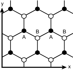
Figure 1: The honeycomb lattice.

A second motivating factor for our work is that the 1D version of our 2D sublattice model studied in this paper is known to be stable to the inclusion of weak short-ranged interactions (which are irrelevant in the RG sense)DSF ; MDH1D . The former model also possesses a strongly-divergent low-energy density of states, with a critically delocalized state at zero energy.BOUCHAUD The robust nature of the 1D critical phase to the inclusion of interaction effects is somewhat counterintuitive, given the picture one has of a large number of states crammed into a very narrow window of energy. In this paper, we will show that this result does not generalize to 2D.

In the present paper, we add to the continuum Dirac description of the disordered honeycomb hopping model generic short-ranged interactions that preserve the chiral symmetry, defined for the Dirac model below in Eq. (8), and in the paragraph following that equation. We use the Schwinger-Keldysh methodKELDYSH to perform the ensemble average over realizations of the disorder. We then employ a one-loop renormalization group treatment to investigate the stability of the disordered, critically delocalized phase to interaction effects. We find that the same mechanism responsible for driving the divergence of the low-energy density of states also feeds into same-sublattice (e.g. next-nearest-neighbor) interactions, producing an instability where the interaction strength grows to large values. We show that this instability always occurs at low enough energies, regardless of whether or not the (non-interacting) disordered system reaches the regime beyond the freezing transition discussed above. We speculate that this instability corresponds to the onset of some kind of Mott insulating phase, dominated by interactions rather than disorder.

Our results are both expected and surprising: expected, because of the strongly divergent density of states and the potentially fragile nature of the low-dimensional, critical disorder-only physics (i.e. in the absence of interactions); surprising, first because, as was already mentioned, the opposite result obtains in 1D, and second because the clean Dirac fixed point is robust against all short-ranged interaction effects. If the observed instability ultimately drives the disordered chiral symmetric model into an interaction-dominated, homogeneous Mott insulating phase, then we have discovered a somewhat curious route: a clean system, initially insensitive to interaction effects, can be made unstable to interactions upon the inclusion of (a special kind of) weak static disorder. One might dub this a “disorder-driven Mott transition.”

The organization of this paper is as follows. In Sec. II we define the honeycomb lattice model and summarize the disordered low-energy effective Dirac theory. We then include short-ranged interactions, and define a set of coupling constants to encode the model physics. In Sec. III, we set up a one-loop renormalization group treatment of the full, disordered and interacting field theory. We re-derive the weak-coupling RG flow equations of the non-interacting, disorder-only modelHWK ; BERNARD ; GLL as a check of our methodology. We then compute the scaling dimensions of the various interaction operators; these scaling dimensions are new. In Sec. IV, we solve the combined RG flow equations for the disorder and interaction couplings, and we interpret the results. The reader less interested in calculational details may skip Sec. III, and proceed from the end of Sec. II directly to Sec. IV.

II MODEL AND SETUP

II.1 Lattice model and continuum limit

Consider a system of spinless fermions at half-filling on the honeycomb lattice with nearest-neighbor hopping. The lattice is depicted in Fig. 1. We define fermion annihilation operators $c_{Ai}$ and $c_{Bj}$ on the “A” and “B” triangular sublattices, respectively; then the random hopping Hamiltonian may be written as

$$H=\sum_{\langle{ij}\rangle}c_{Ai}^{\dagger}\,t_{ij}\,c_{Bj}+h.c.,$$ (3)

where the sum runs over all nearest-neighbor bonds on the honeycomb lattice. We take the hopping amplitudes $t_{ij}$ to be purely real. In the clean limit, $t_{ij}=t$; then the Hamiltonian in Eq. (3) possesses two energy bands of Bloch states indexed over the hexagonal Brillouin zone (Fig. 2), and, as in graphene, the low energy states reside near the corners of the zone where the two bands meet at isolated Fermi points.

We truncate the Bloch spectrum of the clean system to low-energy modes with wavenumbers $\bm{k}=(k_{x},k_{y})$ living within a momentum cutoff $\Lambda$ of the zone corners. Alternate corners are equivalent by reciprocal lattice translations, so we retain modes near two opposite corners, which we index by the Fermi wavevectors $\pm\bm{k_{F}}=(\pm k_{F},0)$, shown in Fig. 2. An effective low-energy Dirac description emerges if we construct the 4-component spinor

$$\psi(\bm{k})\equiv\left[\begin{array}[]{c}c_{A}(\bm{k}+\bm{k_{F}})\\ c_{B}(\bm{k}+\bm{k_{F}})\\ c_{A}(\bm{k}-\bm{k_{F}})\\ c_{B}(\bm{k}-\bm{k_{F}})\end{array}\right],$$ (4)

with $\left|\bm{k}\right|<\Lambda$. Linearizing the energy bands near the Fermi points and incorporating the hopping disorder as a perturbation, we find the non-interacting Hamiltonian

$$H_{D} = -\int d^{2}r\,\psi^{\dagger}(\bm{r})\left[v_{F}\,{\alpha_{\mu}\left(i\,\partial_{\mu}+A_{\mu}\,\beta^{0}\right)}\right]\psi(\bm{r})\quad$$ (5)

$$+\int d^{2}r\,\psi^{\dagger}(\bm{r})\left[m^{i}\beta^{i}\,\right]\psi(\bm{r}),\quad$$

where $v_{F}$ is the Fermi velocity, and $\psi(\bm{r})$ is the long-wavelength Fourier transform of (4). The disorder emerges in the continuum theory (5) as a random vector potential $A_{\mu}(\bm{x})$, $\mu\in\{x,y\}$, and a pair of random Dirac masses $m^{i}(\bm{x})$, $i\in\{1,2\}$. In Eq. (5), summation on repeated indices is implied and will be assumed throughout the rest of the paper.

The symbols $(\alpha_{x},\alpha_{y})$ and $\{\beta^{0},\beta^{1},\beta^{2}\}$ in Eq. (5) denote various 4$\times$4 matrices. Explicit representations can be derived from the honeycomb lattice model. We introduce two sets of Pauli matrices: the matrix $\sigma^{\lambda}$ acts on the sublattice (A-B) space, while the matrix $\tau^{\gamma}$ acts on the Fermi point “flavor” space, with $\lambda,\gamma\in\{1,2,3\}$. Then

$$(\alpha_{x},\alpha_{y}) =(-\sigma^{1}\tau^{3},-\sigma^{2}),$$ (6a)

and

$$\{\beta^{0},\beta^{1},\beta^{2}\} =\{\tau^{3},\sigma^{1}\tau^{1},\sigma^{1}\tau^{2}\}.$$ (6b)

The disordered Dirac Hamiltonian $H_{D}$ given by equation (5) is the most general non-interacting 4-component Dirac Hamiltonian (up to irrelevant terms) consistent with the defining symmetries of the chiral sublattice model. The disordered lattice Hamiltonian defined in Eq. (3) is invariant under time-reversal ($\mathcal{T}$) and chiral ($\mathcal{C}$) transformations. In the continuum theory, these transformations appear as

$$\mathcal{T}:\,\Psi\rightarrow\tau^{1}\Psi,\,i\rightarrow-i$$ (7)

and

$$\mathcal{C}:\,\Psi\rightarrow\sigma^{3}(\Psi^{\dagger})^{T},\,i\rightarrow-i$$ (8)

where $T$ denotes matrix transpose. Note that both the time-reversal and chiral transformations are antiunitary in this language. We stress that in the $2^{nd}$-quantized formulation discussed here, the “chiral symmetry” is represented by the fact that the (second-quantized) Dirac Hamiltonian, given by Eq. (5), is invariant under the transformation defined by Eq. (8). This is easily seen to be equivalent to the first-quantized definition in Eq. (1), above.—The Hamiltonian $H_{D}$ in Eq. (5) was originally derived in the context of the random bond $\pi$-flux model on the square lattice;HWK ; FRADKIN ; LFSG note that on the honeycomb lattice, we obtain the same effective field theory in zero magnetic flux.

We take $A_{\mu}(\bm{x})$ and $m^{i}(\bm{x})$ to be Gaussian white-noise–distributed random variables, and we require that the ensemble-averaged system be invariant under honeycomb lattice rotations, translations, and reflections. These assumptions lead to the conditions

$$\overline{A_{\mu}(\bm{x})}=\overline{m^{i}(\bm{x})}=0,$$ (9)

$$\overline{A_{\mu}(\bm{x})\,A_{\nu}(\bm{x^{\prime}})}=g_{A}\,2\pi\,\delta_{\mu\nu}\delta(\bm{x}-\bm{x^{\prime}}),$$ (10)

and

$$\overline{m^{i}(\bm{x})\,m^{j}(\bm{x^{\prime}})}=g\,2\pi\,\delta^{ij}\delta(\bm{x}-\bm{x^{\prime}}).$$ (11)

In these equations the overbar denotes disorder averaging, and the factors of $2\pi$ are conventional. The disorder-averaged theory is characterized by two parameters, the variances $g$ and $g_{A}$ of the random mass and random vector potential, respectively.

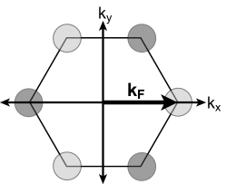
Figure 2: Hexagonal Brillouin zone appropriate to the triangular sublattice. The independent zero energy Fermi points of the honeycomb model occur at $\pm\bm{k_{F}}$; low-energy states have wavenumbers $\bm{k}$ such that $\left|\bm{k}\mp\bm{k_{F}}\right|<\Lambda\ll k_{F}$.

An interpretation of the two types of disorder appearing in Eq. (5) in terms of the physics of the honeycomb lattice model is obtained by examining the structures of the matrices in Eq. (6), used to define them. The random masses couple the two Fermi nodes together in flavor space, while the random vector potential does not. Thus the random mass parameter $g$ characterizes elastic backscattering between the two independent Fermi nodes (involving large crystal momentum transfers), while the random vector potential parameter $g_{A}$ characterizes intranode scattering involving small crystal momentum transfers. As discussed in Sec. I, $g$ turns out to be related to the dimensionless DC resistance, which is independent of $g_{A}$; on the other hand, $g_{A}$ dominates “one-particle” properties, including the density of states.GLL This separation of one and two-particle properties is a characteristic feature of the chiral disorder classes.

II.2 Adding interactions

We complete the setup of our problem in this subsection by adding to the disordered Dirac model [defined by Eq. (5)] generic short-ranged interactions that preserve the chiral (sublattice) symmetry. Consider the set of all four-fermion operators in the low-energy effective continuum theory that are purely local in space and time, and involve no derivatives. All such operators are irrelevant at the clean Dirac fixed point, but comprise the least irrelevant set of local multiparticle interaction terms that we can write down. One then expects that these should be the most important local operators to study once we turn on the disorder. We can enumerate all independent four-fermion terms consistent with (i) the discrete $\mathcal{T}$ and $\mathcal{C}$ symmetries [Eqs. (7) and (8)], and with (ii) the assumptions of statistical invariance under honeycomb rotation, translation, and reflection transformations. It turns out that there are four such local operators; in this subsection, however, we will only discuss two of them in detail. (The other two turn out to be even more irrelevant in the disordered phase than at the clean Dirac fixed point. In Sec. III, below, we will calculate the anomalous dimensions of all four operators.)

Consider the local fermion density operators $n_{Ai}=c_{Ai}^{\dagger}c_{Ai}$ and $n_{Bj}=c_{Bj}^{\dagger}c_{Bj}$ defined on the A and B sublattices of the honeycomb model. In the continuum Dirac theory, we define

$$\bar{\rho}(\bm{r})\equiv\frac{1}{2}\psi^{\dagger}(\bm{r})\left(1+\sigma^{3}\right)\psi(\bm{r})\sim n_{A}(\bm{r})$$ (12a)

and

$$\rho(\bm{r})\equiv\frac{1}{2}\psi^{\dagger}(\bm{r})\left(1-\sigma^{3}\right)\psi(\bm{r})\sim n_{B}(\bm{r}),$$ (12b)

where the identification with the sublattice operators holds up to terms that oscillate on the lattice scale.

The two important four-fermion interactions may be written simply in terms of products of the long-wavelength sublattice density operators defined in Eq. (12). They are $\bar{\rho}\rho(\bm{r})$ on one hand, and $(\bar{\rho}^{2}+{\rho}^{2})(\bm{r})$ on the other. The operator $\bar{\rho}\rho$, which involves a product of the long-wavelength densities from the two different sublattices, can be shown to result from the continuum limit of, for example, nearest-neighbor density-density interactions:

$$\sum_{\langle ij\rangle}\left(n_{Ai}-\textstyle{\frac{1}{2}}\right)\!\left(n_{Bj}-\textstyle{\frac{1}{2}}\right)\sim\int d^{2}r\,\bar{\rho}\rho(\bm{r}).$$ (13)

The other important four-fermion local operator is $\bar{\rho}^{2}+{\rho}^{2}$. Microscopically, the operators $\bar{\rho}^{2}$ and $\rho^{2}$ are pure intrasublattice interactions, i.e. they do not couple together particles on the two different sublattices. These are the only such four-fermion terms that we can write down. Note that invariance under y-axis reflections (which exchange the two sublattices—see Fig. 1) requires $\bar{\rho}^{2}$ and $\rho^{2}$ to appear in the combination $\bar{\rho}^{2}+\rho^{2}$ with identical coefficients. Thus $\bar{\rho}^{2}+{\rho}^{2}$ represents the most relevant piece of arbitrary short-ranged same-sublattice (e.g. next-nearest-neighbor) interactions.

In order to perform the average over disorder realizations, we write a standard $(2+1)$-dimensional (real-)time-ordered ($T$-ordered) Grassmann path integral $Z_{T}$ to represent the disordered Dirac theory. We use the Schwinger-Keldysh methodKELDYSH to normalize this path integral to unity in order to perform the disorder average; in this method, we exploit the fact that the normalization factor $1/Z_{T}$ can be written simply as an anti–time-ordered ($\bar{T}$-ordered) path integral $Z_{\bar{T}}$ for the same theory. This construction works regardless of whether the model includes interparticle interactions or not.

Table 1: Continuum versions of honeycomb lattice model symmetry transformations in the L/R language.

Symmetry	Expression in terms of left(L)- and right(R)-moving components
Chiral ($\mathcal{C}$)	$R(t)\rightarrow-\mu^{1}L(-t)$	$L(t)\rightarrow-\mu^{1}R(-t)$	$\bar{R}(t)\rightarrow\bar{L}(-t)\mu^{1}$	$\bar{L}(t)\rightarrow\bar{R}(-t)\mu^{1}$	$S\rightarrow S^{*}$
Time-reversal ($\mathcal{T}$)	$R(t)\rightarrow-L(-t)$	$L(t)\rightarrow-R(-t)$	$\bar{R}(t)\rightarrow\bar{L}(-t)$	$\bar{L}(t)\rightarrow\bar{R}(-t)$	$S\rightarrow S^{*}$
x-Reflection	$R\rightarrow-L$	$L\rightarrow-R$	$\bar{R}\rightarrow\bar{L}$	$\bar{L}\rightarrow\bar{R}$
y-Reflection	$R\rightarrow-i\mu^{2}\bar{L}^{T}$	$L\rightarrow i\mu^{2}\bar{R}^{T}$	$\bar{R}\rightarrow L^{T}i\mu^{2}$	$\bar{L}\rightarrow-R^{T}i\mu^{2}$
Rotations	$R\rightarrow e^{i\theta}R$	$L\rightarrow e^{-i\theta}L$	$\bar{R}\rightarrow\bar{R}e^{i\theta}$	$\bar{L}\rightarrow\bar{L}e^{-i\theta}$
Translations	$R\rightarrow e^{i\theta}R$	$L\rightarrow e^{-i\theta}L$	$\bar{R}\rightarrow\bar{R}e^{-i\theta}$	$\bar{L}\rightarrow\bar{L}e^{i\theta}$
Electrical charge U(1)	$R\rightarrow e^{i\theta\mu^{3}}R$	$L\rightarrow e^{i\theta\mu^{3}}L$	$\bar{R}\rightarrow\bar{R}e^{-i\theta\mu^{3}}$	$\bar{L}\rightarrow\bar{L}e^{-i\theta\mu^{3}}$

Specifically, we write the theory in terms of the Schwinger-Keldysh generating functional $Z$ defined as (see e.g. Ref. KELDYSH, )

$$Z\equiv Z_{T}Z_{\bar{T}}=\int\mathcal{D}\psi_{a}\,\mathcal{D}\bar{\psi}_{a}\,e^{i\left(S_{D}+S_{I}\right)},$$ (14)

where the non-interacting action $S_{D}$, containing the disorder potentials, is given by

$$S_{D}=\sum_{a=1,2}s_{a}\int d\omega\,d^{2}r\;\bar{\psi}_{a}(\omega,\bm{r})\left[h\,\omega+i\,s_{a}\,\eta\,\operatorname{sgn}(\omega)+{\alpha_{\mu}\left(i\,\partial_{\mu}+A_{\mu}\,\beta^{0}\right)-m^{i}\beta^{i}\,}\right]\psi_{a}(\omega,\bm{r}),$$ (15)

while $S_{I}$ contains the four-fermion interactions

$$S_{I}=-\sum_{a=1,2}s_{a}\int dt\,d^{2}r\left[U\left(\bar{\rho}_{a}^{2}+{\rho}_{a}^{2}\right)\!(t,\bm{r})+W\bar{\rho}_{a}\rho_{a}(t,\bm{r})+X\mathcal{O}^{X}_{a}(t,\bm{r})+Y\mathcal{O}^{Y}_{a}(t,\bm{r})\right].$$ (16)

The integration in Eq. (14) is over the Grassmann fields $\psi_{a}$ and $\bar{\psi}_{a}$, where the (“Keldysh-”) index $a\in\{1,2\}$ denotes the $T$-ordered ($a=1$) or $\bar{T}$-ordered ($a=2$) copy of the theory. The factor $s_{a}$ appearing in the action $S_{D}$ (15) is given by

$$s_{a}=\left\{\begin{array}[]{lll}\phantom{-}1,&a=1&(T\text{-ordered}),\\ -1,&a=2&(\bar{T}\text{-ordered}).\end{array}\right.$$ (17)

The term $i\,s_{a}\,\eta\,\operatorname{sgn}(\omega)$ in $S_{D}$ is the pole-prescription appropriate to $T$ and $\bar{T}$-ordered Green’s functions, with $\eta~{}\rightarrow~{}0^{+}$. In Eq. (15), we have set the Fermi velocity $v_{F}=1$, and the various 4$\times$4 matrices appearing in the theory were defined in Eq. (6). Finally, the coupling constant $h$ in Eq. (15) is a dynamic scale factor, and will be used to track the relationship between length and energy as we renormalize the theory.

In Eq. (16), we have introduced coupling constants $U$ and $W$ for the $\bar{\rho}^{2}+\rho^{2}$ and $\bar{\rho}\rho$ interaction operators, respectively. We denote by $X$ and $Y$ the coupling constants of a pair of additional interaction operators $\mathcal{O}^{X}$ and $\mathcal{O}^{Y}$ that carry the same naive engineering dimension as $\bar{\rho}^{2}+\rho^{2}$ and $\bar{\rho}\rho$. Although these additional operators are required to close the one-loop RG, we do not define them explicitly at this point (but see Sec. III.2.3), because they will turn out to be strongly irrelevant in the disordered phase. To simplify notation, we define the vector of interaction couplings

$$\vec{U}\equiv\{U,\,W,\,X,\,Y\}.$$ (18)

The expressions for the Schwinger-Keldysh path integral $Z$ [Eq. (14)] and the action $S_{D}+S_{I}$ [Eqs. (15) and (16)] constitute the completed formulation of the full, interacting and disordered fermion problem with chiral symmetry. Upon averaging over realizations of the disorder potentials $m^{i}$ and $A_{\mu}$, we find that the theory requires the specification of a total of seven coupling constants: the random mass and random vector potential variances $g$ and $g_{A}$, the four interaction strengths $\vec{U}$, and finally the dynamic scale factor $h$. In the next section we perform a perturbative one-loop RG analysis on this model. The principal new results are the scaling behaviors of the interaction couplings $\vec{U}$ as we look at lower and lower energies, or, equivalently, larger and larger values of the flowing coupling $g_{A}$. The reader interested only in our results may skip directly to Sec. IV, where the scaling behaviors of the various couplings are simply stated and analyzed.

III ONE-LOOP CALCULATION

In this section we perform a one-loop renormalization group analysis on the interacting and disordered chiral fermion model defined in Sec. II. We begin by re-writing the Grassmann Dirac field appearing in the Keldysh path integral [Eq. (14)] in terms of “left(L)-” and “right(R)-moving” components, inspired by a similar decomposition made for the non-interacting system in Ref. GLL, . (This L/R decomposition provides a language similar to that used in Ref. MRF, to investigate the freezing transition in the dynamic critical exponent and the low-energy density of states.) We then perform a hard cutoff field theory renormalization group analysis to one loop. The L/R formulation allows for a particularly simple and transparent treatment using diagrams. With a minimal effort we recover, as a check, the one-loop RG results for the disorder-only modelHWK ; BERNARD ; GLL [Eqs. (40, 43, 45)]. Finally, we calculate the anomalous dimensions of all allowed four-fermion interaction operators in the presence of the disorder [Eqs. (51, 52, 53, 55)].

III.1 Left(L)/Right(R) decomposition

Consider the Keldysh action for the non-interacting disordered chiral system, given in Eq. (15). We make the basis change [$a=1,2$ is the Keldysh-index; Eqs.(15,16)]

$$\psi_{a}\rightarrow U\,\psi_{a},\,\bar{\psi}_{a}\rightarrow\bar{\psi}_{a}\,U^{\dagger},$$ (19)

where the unitary matrix $U$ is

$$U\equiv U_{p}\,\textstyle{\frac{1}{\sqrt{2}}}\left(1+i\sigma^{2}\tau^{3}\right)\,\textstyle{\frac{1}{\sqrt{2}}}\left(1-i\sigma^{2}\right).$$ (20)

Here $U_{p}\equiv(1/2)\left(1+{\vec{\sigma}}\cdot{\vec{\tau}}\right)$ is the permutation operator, exchanging $\sigma^{\alpha}\leftrightarrow\tau^{\alpha}$ upon conjugation. This basis change induces a similarity transformation on the matrices defined in Eq. (6); the transformed versions are $\bm{\alpha}=~{}(\alpha_{x},\alpha_{y})=~{}(\sigma^{1}\tau^{1},\sigma^{2}\tau^{1})$ and $\{\beta^{0},\beta^{1},\beta^{2}\}=~{}\{\sigma^{3}\tau^{3},\sigma^{3}\tau^{1},\tau^{2}\}$.

Following Ref. GLL, , we define the L/R decomposition of the Dirac spinors:

$$\psi_{a} \equiv \left[\begin{array}[]{c}\bar{L}_{2a}\\ \bar{R}_{2a}\\ L_{1a}\\ R_{1a}\end{array}\right]$$ (25)

and

$$\bar{\psi}_{a}\equiv s_{a}\left[\bar{R}_{1a}\,\bar{L}_{1a}\,R_{2a}\,L_{2a}\right],$$ (26)

where the first index $i\in\{1,2\}$ on the components $R_{ia}$ and $L_{ia}$ is a species index. Thus the fields $R_{a}$ (“right-movers”) and $L_{a}$ (“left-movers”) are two-component objects. In terms of the latter, the non-interacting action given by Eq. (15) may now be written very simply as

$$S_{D}= i\,\int dt\,d^{2}r\left[h\,\left(\bar{R}_{a}\mu^{1}\partial_{t}\bar{L}^{T}_{a}\right)+h\,\left(L^{T}_{a}\mu^{1}\partial_{t}R_{a}\right)+\bar{R}_{a}(\partial-A)R_{a}+\bar{L}_{a}(\bar{\partial}-\bar{A})L_{a}\right.$$ (27)

$$\left.+m\,\bar{R}_{a}L_{a}+\bar{m}\,\bar{L}_{a}R_{a}\right].$$

where the Pauli matrix $\mu^{1}$ is a matrix in the species space of the Fermion fields [which is the first index $i$ of Eqs. (25) and (26)].

In equation (27) we have suppressed the $T$ and $\bar{T}$-ordering pole prescriptions [Eq.(15)], and we have introduced the following complex notations: (i) $\partial\equiv\partial_{x}-i\partial_{y}$ and $\bar{\partial}\equiv\partial_{x}+i\partial_{y}$, (ii) $A\equiv A_{y}+iA_{x}$ and $\bar{A}\equiv A_{y}-iA_{x}$ and (iii) $m\equiv m^{2}+im^{1}$ and $\bar{m}\equiv m^{2}-im^{1}$.

Turning to the interactions, we seek the set of all independent four-fermion operators local in space and time with no derivatives; as discussed in subsection II.2, these operators form a set of local perturbations least irrelevant at the clean Dirac fixed point. Any allowed interaction operator must be invariant under discrete chiral, time-reversal, and spatial reflection operations, and it must also transform as a singlet under continuous U(1) “electrical charge”, rotation, and honeycomb lattice translation transformations. We summarize the action of these symmetry transformations in the above L/R basis of low-energy fields in Table 1. Consistent with these requirements, we find the four independent local four-fermion operators

$$\mathcal{O}^{A}_{a} \equiv (\bar{R}_{a}\frac{\mu^{1}}{2}R_{a})\,(\bar{L}_{a}\frac{\mu^{1}}{2}L_{a})+(\bar{R}_{a}\frac{\mu^{2}}{2}R_{a})\,(\bar{L}_{a}\frac{\mu^{2}}{2}L_{a}),\qquad$$

$$\mathcal{O}^{B}_{a} \equiv (\bar{R}_{a}\frac{\mu^{3}}{2}R_{a})\,(\bar{L}_{a}\frac{\mu^{3}}{2}L_{a}),$$ (28b)

$$\mathcal{O}^{C}_{a} \equiv -\frac{(\bar{R}_{a}R_{a})}{2}\,\frac{(\bar{L}_{a}L_{a})}{2},$$ (28c)

and

$$\mathcal{O}^{U}_{a}\equiv\bar{\rho}_{a}^{2}+\rho_{a}^{2},$$ (29)

where

$$\bar{\rho}_{a} = i(\bar{L}_{a}\mu^{2}\bar{R}_{a}^{T}),$$ (30a)

$$\rho_{a} = -i(R_{a}^{T}\mu^{2}L_{a}).$$ (30b)

Equation (30) gives the L/R language expressions for the long-wavelength sublattice density operators defined by Eq. (12). The operator $\mathcal{O}^{U}_{a}$ given by Eq. (29) is one of the two four-fermion interaction terms that will turn out to be more relevant in the disordered critical phase than at the clean Dirac fixed point; the other, $\bar{\rho}_{a}\rho_{a}$, can be written in terms of the three operators defined in Eq. (28):

$$\bar{\rho}_{a}\rho_{a}=-2\left(\mathcal{O}^{A}_{a}+\mathcal{O}^{B}_{a}+\mathcal{O}^{C}_{a}\right).$$ (31)

Note that the three operators in Eq. (28), as well as the whole structure of the non-interacting theory [Eq. (27)] except the “energy” terms (the terms involving time derivatives) are invariant under a U(1) transformation, which we refer to as a “sublattice” U(1),

$$R_{a}\rightarrow e^{i\theta}R_{a},\,L_{a}\rightarrow e^{i\theta}L_{a},\,\bar{R}_{a}\rightarrow\bar{R}_{a}e^{-i\theta},\,\bar{L}_{a}\rightarrow\bar{L}_{a}e^{-i\theta}.$$ (32)

(distinct from the “electrical charge” U(1) defined in Table I). This U(1) transformation is not a symmetry, because the energy terms in the non-interacting action carry non-zero (i.e. unit) charge. In fact, under this $U(1)$, the two energy terms $i(\bar{R}_{a}\mu^{1}\partial_{t}\bar{L}_{a}^{T})$ and $i(L_{a}^{T}\mu^{1}\partial_{t}R_{a})$ carry equal and opposite unit charges, as do the local sublattice density operators $\bar{\rho}_{a}$ and $\rho_{a}$, while the four-fermion interaction operator $\mathcal{O}_{a}^{U}$ [Eq. (29)] is a sum of positive and negative doubly-charged same-sublattice components.

Figure 3: Feynman rules for the diagrams in Fig. 4.

In the non-interacting disordered fermion problem, moments of the local density of states (LDOS) operator are known to exhibit negative scaling dimensions in the disordered, critically delocalized phase.GLL ; MRF [The LDOS operator appears in the (2+1)D Keldysh formulation as the Dirac fermion bilinear $\bar{\psi}_{a}(\omega,\bm{r})\psi_{a}(\omega,\bm{r})$, which is local in position space and frequency but not in time.] More precisely, it is the components of these LDOS moments with maximal charge under the sublattice U(1) transformation defined by Eq. (32) that carry the maximally negative scaling dimensions, i.e. these components are the most relevant perturbations to the zero-energy nearly conformal field theory. The functional RG treatment employed in Ref. MRF, focuses just upon these most relevant components of the LDOS moments in order to extract the dynamic critical exponent in the regime above the freezing transition. In our interacting problem, we will find that the interaction operator $\mathcal{O}_{a}^{U}=\bar{\rho}_{a}^{2}+\rho_{a}^{2}$, which is maximally-charged under the “sublattice” U(1), is the most relevant of the investigated four-fermion interaction terms. Note that unlike the LDOS operator or the energy terms in the non-interacting action (27), the sum of sublattice density operators $\bar{\rho}_{a}+\rho_{a}$ cannot receive any corrections to scaling: this local spacetime operator is a component of the $(2+1)$-dimensional conserved “electrical charge” U(1) current carried by the electrically-charged Dirac fermions [Table I].

Next we average the Keldysh functional $Z$ [Eq. (14)] over realizations of the random vector potential $A=A_{x}+iA_{y}$ and the complex random mass $m$, with $\overline{\bar{A}(\bm{x})\,A(\bm{x^{\prime}})}=4\pi g_{A}\,\delta(\bm{x}-\bm{x^{\prime}})$ and $\overline{\bar{m}(\bm{x})\,m(\bm{x^{\prime}})}=4\pi g\,\delta(\bm{x}-\bm{x^{\prime}})$. The resulting non-interacting disorder-averaged action $\overline{S_{D}}$ may be written in its final form as a sum of two terms: $\overline{S_{D}}\equiv S_{D}^{\,0}+\overline{\delta S_{D}}$, where

$$S_{D}^{\,0}=i\,\int dt\,d^{2}r\left[\bar{R}_{a}\,L_{a}^{T}\right]\left[\begin{array}[]{cc}\partial&h\,\mu^{1}\partial_{t}\\ h\,\mu^{1}\partial_{t}&\bar{\partial}\end{array}\right]\left[\begin{array}[]{c}R_{a}\\ \bar{L}_{a}^{T}\end{array}\right]\qquad$$ (33)

and

$$\overline{\delta S_{D}}=-4\pi i\int dt\,dt^{\prime}\,d^{2}r \left[g\,(\bar{R}_{a}L_{a})(t)\,(\bar{L}_{b}R_{b})(t^{\prime})\right.$$ (34)

$$\left.+g_{A}\,(\bar{R}_{a}R_{a})(t)\,(\bar{L}_{b}L_{b})(t^{\prime})\right].\quad$$

The average over disorder has coupled together fermion bilinears with different Keldysh indices at arbitrarily distant times.

Figure 4: Diagrams renormalizing the self-energy.

III.2 Perturbative analysis

We calculate one-loop corrections to the propagators in (33) and to the disorder vertices in (34), and we compute the anomalous dimensions of the interaction operators given by Eqs. (28) and (29). The dependence of these corrections on a hard momentum cutoff $\Lambda$ will be usedDJA to derive the renormalization group equation summarized in Sect. IV.

III.2.1 Self-energy

In order to calculate the self-energy, it is useful to define the fields $\chi_{a}$ and $\bar{\chi}_{a}$ via [Keldysh index $a\in\{1,2\}$]

$$\chi_{a}\equiv\left[\begin{array}[]{c}R_{a}\\ \bar{L}_{a}^{T}\end{array}\right]$$ (35)

and

$$\bar{\chi}_{a}\equiv\left[\bar{R}_{a}\,L_{a}^{T}\right].$$ (36)

We can think of $\chi_{a}\equiv\left\{\chi_{\gamma a}\right\}_{\gamma}$ as a 2-component R/L-valued object; the index $\gamma\in\{R,L\}$ addresses the two components of the definition in Eq. (35); each field $R_{a}$ or $\bar{L}_{a}$ carries in addition a 2-component species index $i$, defined in Eq. (25). ($\chi_{\gamma ia}$ when all indices are displayed.)

The propagator for the field $\chi_{a}$ follows from Eq. (33), and is given by

$$\left\langle\chi_{a}(\omega,\bm{k})\bar{\chi}_{a}(\omega,\bm{k})\right\rangle=\frac{-i}{\bar{k}k-h^{2}(\omega^{2}+i\eta s_{a})}\begin{bmatrix}\bar{k}&h\omega\mu^{1}\\ h\omega\mu^{1}&k\end{bmatrix}\!\!,$$ (37)

where $k\equiv k_{x}-ik_{y}$ and $\bar{k}\equiv k_{x}+ik_{y}$. In Eq. (37) we have restored the correct $T$ and $\bar{T}$-ordering pole prescriptions in the two Keldysh species. We can also re-write the disorder-averaged action $\overline{\delta S_{D}}$ given by Eq. (34) in terms of the $\chi_{\gamma a}$ fields [“T” denoting the transpose, and $\gamma\in\{L,R\}$]:

$$\overline{\delta S_{D}}=-4\pi i\int dt\,dt^{\prime}\,d^{2}r\left[g\,(\bar{\chi}_{Ra}\,\bar{\chi}_{La}^{T})(t)\,(\chi_{Lb}^{T}\,\chi_{Rb})(t^{\prime})\right.$$ (38)

$$\left.-g_{A}\,(\bar{\chi}_{Ra}\,\chi_{Ra})(t)\,(\bar{\chi}_{Lb}\,\chi_{Lb})(t^{\prime})\right].\quad$$

We depict the disorder vertices $g$ and $g_{A}$ with dashed lines, shown in Fig. 3.

Figure 4 shows the one-loop disorder contributions to the self-energy. In these diagrams the propagator $\left\langle\chi_{\gamma}\bar{\chi}_{\gamma^{\prime}}\right\rangle$ is represented as a directed solid line labeled with the endpoint indices $(\gamma,\,\gamma^{\prime})\in\{R,L\}$. (Keldysh indices are suppressed.) We furnish the external $\chi$ field legs with the labels “R” and “L” to indicate which propagator is being corrected.

Figure 5: Feynman rules for the diagrams in Figs. 6—9. The interaction vertex labeled $\mathcal{O}^{M}$ denotes the sublattice U(1) charge-neutral operators defined by Eq. (28), while the vertex labeled $\mathcal{O}^{U}$ depicts the $\bar{\rho}^{2}$ component of the sublattice-charged interaction operator $\bar{\rho}^{2}+{\rho}^{2}$.

The two diagrams appearing in Fig. 4(a) correspond to the one-loop self-energy corrections to $\left\langle\chi_{R}\bar{\chi}_{R}\right\rangle$. Both of these diagrams vanish: the first diagram contributes nothing because it contains a free Keldysh index summation,KELDYSH while the second diagram vanishes because the momentum integral of the purely left-moving propagator $\left\langle\chi_{L}\bar{\chi}_{L}\right\rangle$ gives zero. Thus we find that there is no self-energy correction to the “R-R” sector of the $\chi$ field propagator to one-loop order.

By contrast, the diagrams contributing to the self-energy correction to $\left\langle\chi_{R}\bar{\chi}_{L}\right\rangle$ shown in Fig. 4(b) lead to a non-zero renormalization of the dynamic scale factor $h$. The irreducible two-point vertex function in this channel to one loop is [cf.  Eq. (37)]

$$\Gamma_{RL}(\omega,\bm{k})=ih\omega\mu^{1}[1+2(g+g_{A})\ln\Lambda],$$ (39)

where $\Lambda$ is an ultraviolet momentum cutoff and we did not write out ultraviolet-finite corrections. Differentiating Eq. (39) with respect to $\ln\Lambda$ and setting the result equal to zero leads to the expressionDJA

$$\left(\frac{d\ln h}{dl}\right)_{an}=2(g+g_{A}),$$ (40)

where $l\equiv-\ln\Lambda$ is the logarithm of the RG length scale. The subscript “$an$” appearing on the left hand side of Eq. (40) stands for “anomalous,” as the above calculation has given us only the anomalous part of the beta function; in order to obtain the full one-loop flow equation for $h$, we must add the appropriate “engineering dimension” to Eq. (40). This will be done in Sec. IV, below.

Although we have considered the propagator renormalization due only to the disorder, it can be easily seen that none of the local spacetime interaction operators defined in Eqs. (28) and (29) can generate a non-zero one-loop contribution to the Dirac field self-energy; such a contribution would necessarily correspond to either the generation of a mass or a chemical potential shift, both forbidden by symmetry.

III.2.2 Disorder self-renormalization

Next we turn to the self-renormalization of the disorder couplings $g$ and $g_{A}$. We will only need the diagonal components of the propagator given by Eq. (37), so we revert back to the $\{R,L,\bar{R},\bar{L}\}$ component language [the species index $i=1,2$, Eq. (25, 26), will be suppressed]. The propagators we will need are

$$\left\langle R_{a}(\omega,\bm{k})\bar{R}_{a}(\omega,\bm{k})\right\rangle=\frac{-i\bar{k}}{\bar{k}k-h^{2}(\omega^{2}+i\eta s_{a})}$$ (41)

and

$$\left\langle L_{a}(\omega,\bm{k})\bar{L}_{a}(\omega,\bm{k})\right\rangle=\frac{-ik}{\bar{k}k-h^{2}(\omega^{2}+i\eta s_{a})}.$$ (42)

Note that both propagators are odd under the exchange $k\rightarrow-k$.

Now we will use directed solid and dotted lines to depict the $\left\langle R\bar{R}\right\rangle$ and $\left\langle L\bar{L}\right\rangle$ propagators, respectively. We will continue to use dashed lines to indicate the disorder vertices $g$ and $g_{A}$, as shown in Fig. 5(a).

Figure 6: Diagrams renormalizing $g$.

Figure 6 shows the corrections to the $g$ vertex in Eq. (34). The $\ln\Lambda$ contributions due to the first two diagrams exactly cancel those of the second two, leading to the anomalous part of the one-loop beta function

$$\left(\frac{dg}{dl}\right)_{an}=0.$$ (43)

The cancelation is easily understood if one notes that all four diagrams in Fig. 6 contain a closed momentum loop integration involving one of each diagonal propagator given by Eqs. (41) and (42). All four diagrams contribute the same absolute ultraviolet-divergent amplitude to the sum. Note that the loop momentum necessarily flows against one of the two directed chiral propagator arrows in the first pair of diagrams in Fig. 6. In the second pair of diagrams, the loop momentum can be taken to flow in the same direction as both L- and R-propagator arrows. This simple structural difference produces a relative minus sign, forbidding the coupling $g_{A}$ from feeding into $g$. The same mechanism will lead to cancelations in the autorenormalization of $g_{A}$ as well as in the computation of the anomalous dimensions of some of the interaction operators.

In Figure 7, we depict the one-loop disorder-disorder diagrams that renormalize the coupling $g_{A}$. The first two diagrams, each proportional to $g_{A}^{2}$, exactly cancel via the mechanism described above. The third diagram is non-zero, and leads to the irreducible four-point vertex function

$$\Gamma_{g_{A}}=g_{A}+2g^{2}\ln\Lambda.$$ (44)

Differentiation with respect to $l=-\ln\Lambda$ produces the anomalous part of the one-loop beta function

$$\left(\frac{dg_{A}}{dl}\right)_{an}=2g^{2}.$$ (45)

Figure 7: Diagrams renormalizing $g_{A}$.

III.2.3 Interaction operator anomalous dimensions

Finally, we turn to the one-loop calculation of the anomalous dimensions of the four interaction operators defined in Eqs. (28) and (29) in the disordered (critical) phase characterized by finite $g$ and $g_{A}$. The results are listed in Eqs. (51, 52, 53, 55) and Eqs. (64a, 64b, 64c, 64d).

Consider first the three “sublattice-U(1)” charge-neutral interaction operators defined in Eq. (28). We will use a wavy line to represent all three interaction operators simultaneously, as depicted by the vertex labeled $\mathcal{O}^{M}$ in Fig. 5(b); these operators differ only in their species index structure. Figure 8 shows the one-loop renormalization of these interaction operators due to the disorder vertices $g$ and $g_{A}$. The labels $i,j$ and $k,l$ appearing on the external legs denote the species components of the outgoing and incoming right and left-moving particles, respectively. The first four diagrams describe the $g_{A}$-dressing of the interactions; these diagrams cancel up to ultraviolet-finite contributions. The final two diagrams in Fig. 8 involve the $g$ disorder vertex and add constructively. Let us denote the zeroth order irreducible four-point vertex function for the interaction operator $\mathcal{O}^{M}$ via

$$\Gamma^{\,0}_{M\,ij;kl}\equiv\sum_{\lambda}M_{ij}^{\lambda}M_{kl}^{\lambda}.$$ (46)

In this equation, the vertex matrices $M^{\lambda}$ depend upon the operator in question, e.g. the operator $\mathcal{O}^{A}$ [Eq. (28a)] has two such vertex matrices, $M^{1}=\mu^{1}/2$ and $M^{2}=\mu^{2}/2$. Incorporating the correction due to $g$, we find the one-loop irreducible four-point vertex function for the operator $\mathcal{O^{M}}$

$$\Gamma_{M\,ij;kl}=\sum_{\lambda}M_{ij}^{\lambda}M_{kl}^{\lambda}-4g\ln\Lambda\sum_{\lambda}M_{il}^{\lambda}M_{kj}^{\lambda}.$$ (47)

We have such a vertex function for each of the three operators defined in Eq. (28).

Figure 8: Diagrams renormalizing the interaction operators defined by Eq. (28).

We rewrite Eq. (47) using the Pauli matrix identities

$$\mu^{1}_{il}\mu^{1}_{kj}+\mu^{2}_{il}\mu^{2}_{kj}=\delta_{ij}\delta_{kl}-\mu^{3}_{ij}\mu^{3}_{kl},$$ (48a)

$$\mu^{3}_{il}\mu^{3}_{kj}=-\textstyle{\frac{1}{2}}\left(\mu^{1}_{ij}\mu^{1}_{kl}+\mu^{2}_{ij}\mu^{2}_{kl}\right)+\textstyle{\frac{1}{2}}\left(\delta_{ij}\delta_{kl}+\mu^{3}_{ij}\mu^{3}_{kl}\right),$$ (48b)

and

$$\delta_{il}\delta_{kj}=\textstyle(\frac{1}{2})\left(\delta_{ij}\delta_{kl}+\mu^{\alpha}_{ij}\mu^{\alpha}_{kl}\right),$$ (48c)

where in this last identity $\alpha$ is summed over $\{1,2,3\}$. Using these identities with Eq. (47) shows us that the interaction operators mix under disorder-renormalization, leading to the matrix vertex equation

$$\left[\begin{array}[]{c}\Gamma_{A}\\ \Gamma_{B}\\ \Gamma_{C}\end{array}\right]=\left[\begin{array}[]{ccc}1&2c&2c\\ c&1-c&c\\ c&c&1-c\end{array}\right]\left[\begin{array}[]{c}\Gamma^{\,0}_{A}\\ \Gamma^{\,0}_{B}\\ \Gamma^{\,0}_{C}\end{array}\right],$$ (49)

where the constant $c\equiv 2g\ln\Lambda$.

The eigenvalues of the matrix in Eq. (49) determine the anomalous dimensions of the RG eigenoperators, which are linear combinations of the interaction operators defined in Eq. (28). These eigenvalues are $1+4g\ln\Lambda$ and $1-4g\ln\Lambda$; the latter is doubly degenerate. The eigenoperator corresponding to the eigenvalue $1+4g\ln\Lambda$ is

$$\mathcal{O}^{A}+\mathcal{O}^{B}+\mathcal{O}^{C}\propto\bar{\rho}\rho.$$ (50)

If we add this interaction operator to the action of the theory with a coupling constant $W$, as in Eq. (16), then we find the anomalous part of the beta function for $W$

$$\left(\frac{dW}{dl}\right)_{an}=4gW,$$ (51)

making the interaction coupling $W$ more relevant in the (critical) disordered phase than at the clean Dirac fixed point. The other two eigenoperators share the RG eigenvalue $1-4g\ln\Lambda$; if we assign these operators the coupling constants $X$ and $Y$, then we have

$$\left(\frac{dX}{dl}\right)_{an}=-4gX,$$ (52)

and

$$\left(\frac{dY}{dl}\right)_{an}=-4gY,$$ (53)

so that the couplings $X$ and $Y$ turn out to be more irrelevant in the presence of disorder.

Figure 9: Diagrams renormalizing the interaction operator $\bar{\rho}^{2}$.

Finally, we turn to the same-sublattice interaction operator $\mathcal{O}^{U}$ given by Eq. (29). We will use diagrams to compute the renormalization of the $\bar{\rho}^{2}$ half of this operator; the other half $\rho^{2}$ must renormalize the same way. Using Eq. (30), we write $\bar{\rho}^{2}=-\left(\bar{L}_{a}\mu^{2}\bar{R}_{a}^{T}\right)^{2}\propto\bar{L}_{1a}\bar{L}_{2a}\bar{R}_{1a}\bar{R}_{2a}$. We will depict the interaction $\bar{\rho}^{2}$ as a wavy line again joining right and left-mover lines, but now all such lines are directed outwards from the vertex—this half of the interaction operator is a source of “sublattice” U(1) current [see Fig. 5(b)].

The diagrams describing the disorder-dressing of the $\bar{\rho}^{2}$ operator are shown in Fig. 9. Numerical labels on the external legs again refer to the species index $i,j=\{1,2\}$. The first four diagrams involve dressing by the $g_{A}$ vertex. The key point is that these four diagrams add constructively for this sublattice-charged interaction: $g_{A}$ feeds into the operator $\bar{\rho}^{2}$. The cancelation that occured for the sublattice charge-neutral operators given by Eq. (28) does not occur here, because all four diagrams proportional to $g_{A}$ involve a loop momentum that necessarily flows against one of the two directed propagator arrows in that loop. The final two diagrams in Fig. 9 depict the $g$-renormalization of the interaction. Summing these contributions we obtain the irreducible four-point vertex function for the interaction operator $\mathcal{O}^{U}=\bar{\rho}^{2}+\rho^{2}$ to one loop

$$\Gamma_{U}=1+4\left(2g_{A}-g\right)\ln\Lambda.$$ (54)

Adding $\mathcal{O}^{U}$ to the action with coupling $U$ as in Eq. (16), we find the anomalous part of the beta function for the coupling $U$ given by

$$\left(\frac{dU}{dl}\right)_{an}=4\left(2g_{A}-g\right)U.$$ (55)

IV RESULTS AND DISCUSSION

IV.1 Scaling equations

In this section we summarize the scaling behaviors of the coupling constants for the model defined by Eqs. (14), (15), and (16) in Sec. II. Seven coupling constants are needed to describe that model: these are the disorder variances $g$ and $g_{A}$, the interaction strengths $\vec{U}~{}=~{}\left\{U,\,W,\,X,\,Y\right\}$, and the dynamical scale factor $h$. We may extract the full RG beta functions for these couplings by combining the results of Sec. III with dimensional analysis, yielding the “engineering dimensions.” Examine the action for the theory given by Eqs. (15) and (16). We take the dependence of the energy “$\omega$” upon the RG scale factor “$l$” [the logarithm of the (spatial) length scale] to be

$$\frac{d\ln\omega}{dl}\equiv z(l),$$ (56)

In Eq. (56), $z$ is the (possibly scale-dependent) “dynamic critical exponent.” We say that energy has the “engineering dimension”

$$\left[\omega\right]=z$$ (57)

in inverse length units. We take the Fermi velocity $v_{F}=1$ to be dimensionless; then, from Eq. (15), the Dirac field has the engineering dimension

$$\left[\psi(t,\bm{r})\right]=\frac{1+z}{2},\qquad\left[\psi(\omega,\bm{r})\right]=\frac{1-z}{2},$$ (58)

in two spatial dimensions. We then find that the disorder strengths $g$ and $g_{A}$ are dimensionless, the interaction couplings $\vec{U}$ share the engineering dimension

$$[\vec{U}]=-z,$$ (59)

and the dynamic scale factor $h$ has the dimension

$$\left[h\right]=1-z.$$ (60)

Combining the anomalous dimensions in Eqs. (40), (43), (45), (51-53), and (55) from Sec. III with the above engineering dimensional analysis, we find the one-loop flow equations

$$\frac{d\ln h}{dl} =(1-z)+2(g_{A}+g)$$

$$\phantom{==}+\mathcal{O}(g^{2},gg_{A},g\vec{U},g_{A}\vec{U},\vec{U}^{2}),$$ (61)

$$\frac{dg}{dl} =0+\mathcal{O}(g\vec{U},g^{3}),$$ (62)

and

$$\frac{dg_{A}}{dl} =2g^{2}+\mathcal{O}(g_{A}\vec{U},g^{3}),$$ (63)

for the parameters that appear in the non-interacting sector of the theory, and

$$\frac{dU}{dl} =(-z+8g_{A}-4g)U+\mathcal{O}(\vec{U}^{2},g^{2}U,gg_{A}U)$$ (64a)

$$\frac{dW}{dl} =(-z+4g)W+\mathcal{O}(\vec{U}^{2},g^{2}W)$$ (64b)

$$\frac{dX}{dl} =(-z-4g)X+\mathcal{O}(\vec{U}^{2},g^{2}X)$$ (64c)

as well as

$$\frac{dY}{dl} =(-z-4g)Y+\mathcal{O}(\vec{U}^{2},g^{2}Y),$$ (64d)

for the interactions.

In Eqs. (61-63) and (64), the RG function $z(l)$ is so far undetermined. We may choose $z$ any way we like; different choices correspond to different ways of rescaling energy in the (2+1)D field theory after performing the RG transformation. The natural choice

$$\frac{d\ln h}{dl}\equiv 0,$$ (65)

eliminates the parameter $h$ from the theory. Enforcing Eq. (65) order by order in perturbation theory uniquely determines $z$; to one loop, we find that

$$z(l)=1+2(g_{A}+g).$$ (66)

First, note (as a check) that we recover the known resultsHWK ; BERNARD ; GLL (62), (63), and (66) for the non-interacting sector of the theory: the random mass variance $g$ is purely marginal to one loop; by contrast, $g_{A}$ is driven to strong coupling by $g\neq 0$; the scale-dependent dynamic critical exponent $z$ is fed by both $g$ and $g_{A}$.

The scaling behaviors of the interaction couplings given in Eq. (64) are new and will be analyzed below. We stress that the terms maintained in the flow equations (62-64) and (66) are only those required to determine the stability of the non-interacting phase.

Now we address an immediate concern: we are interested in the disordered critical phase that occurs near zero energy as $g_{A}$ flows away from the clean Dirac fixed point (where $g=g_{A}=0$) to strong coupling; this flow always occurs for $g\neq 0$. The reader should therefore question the value of the purely perturbative one-loop results that we have presented above; naively, these lowest order results cannot be trusted to tell us anything about the strong coupling large-$g_{A}$ regime.

Nevertheless, we can safely extend our results to large values of the random vector potential variance $g_{A}\gg 1$; in order to do so, we rely upon several known exact results for the disorder-only modelGLL ; MRF . In the absence of interactions, the exact flow equation for $g$ is strictly zero, while the exact flow equation for $g_{A}$ depends only upon $g$ and vanishes for $g=0$. The exact flow equation for the dynamical exponent $z$ below the freezing transition is linear in $g_{A}$, with non-linear $g$-dependent coefficients. Equations (63) and (66) give the correct behaviors to lowest order in $g$. In this paper, we imagine tuning $g\ll 1$; then our results in fact tell the whole story for the couplings $g$ and $g_{A}$, and for the dynamic critical exponent $z$. (Above the freezing transition, with $g_{A}>g_{A}^{\,c}$, we will need to be more careful—see below.)

Indeed, the scaling dimensions of the important four-fermion interaction operators $\bar{\rho}^{2}+\rho^{2}$ and $\bar{\rho}\rho$, given to one loop in Eqs. (64a) and (64b), respectively (the terms linear in $\vec{U}$), must be exactly linear in $g_{A}$, with higher-loop corrections only modifying their $g$-dependences. These scaling dimensions combine the engineering dimension “$-z$” in these equations with the anomalous dimensions calculated in Sec. III. The anomalous dimensions characterize the disorder-dressing of the interaction operators at zero interaction coupling, and could alternatively be calculated in the $(2+0)$D (non-interacting) version of the theory. Such a calculation in the $(2+0)$D theory can be performed non-perturbatively in $g_{A}$GLL ; MRF ; the anomalous dimension of a local operator in this $(2+0)$D theory is guaranteed to be linear in $g_{A}$ with a coefficient determined by the “sublattice” [Eq. (32)] and “translation” [see Table 1] U(1) charges carried by that operator. Therefore our results in Eqs. (64a) and (64b) are in fact valid to all orders in $g_{A}$. Eqs. (64a) and (64b) incorporate, in addition, the lowest order corrections in $g$.

In the following, we will analyze our results. We note from Eq. (64) that the interaction couplings $U$ and $W$ are enhanced by the disorder, while $X$ and $Y$ are (weakly) suppressed relative to the clean Dirac fixed point. We therefore focus our attention upon the former pair of interactions. Integrating the flow equations (64a) and (64b), we find using Eq. (55)

$$U(l) \sim\left(\frac{\omega(0)}{\omega(l)}\right)\exp\left[\int^{l}_{0}dl^{\prime}\left({\frac{dU}{dl^{\prime}}}\right)_{an}\right]$$

$$\sim\left(\frac{\omega(0)}{\omega(l)}\right)\exp\left[2(2g\,l)^{2}+(8g_{A}^{\,0}-4g)l\right]$$ (67)

and using Eq. (51)

$$W(l) \sim\left(\frac{\omega(0)}{\omega(l)}\right)\exp\left[\int^{l}_{0}dl^{\prime}\left({\frac{dW}{dl^{\prime}}}\right)_{an}\right]$$

$$\sim\left(\frac{\omega(0)}{\omega(l)}\right)\exp\left[4g\,l\right],$$ (68)

where we take $g_{A}^{\,0}\ll 1$ as the bare value of $g_{A}$. In order to derive Eqs. (IV.1) and (IV.1), we have integrated the flow equations for $g$ and $g_{A}$ given by Eqs. (62) and (63).

To complete the story, we need the relationship between the energy $\omega(l)$ and the RG parameter $l$; we obtain this by integrating Eq. (66). We solve the resulting equation for $l$ in terms of $\ln\omega$, where $\omega=\omega(0)$ is the bare energy scale. The result is

$$l\sim\frac{1}{(2g)^{2}} \left\{-1-2\left(g+g_{A}^{\,0}\right)\phantom{\sqrt{\left[g_{A}^{\,0}\right]^{2}}}\right.$$ (69)

$$\left.+\sqrt{\left[1+2\left(g+g_{A}^{\,0}\right)\right]^{2}+8g^{2}\left|\ln\frac{\omega}{\Omega}\right|}\right\},\qquad$$

where $\Omega\equiv\omega(l)\geq\omega$ is an arbitrary finite reference energy. We will state all of our results in terms of the bare energy $\omega\rightarrow 0$, so it is useful to note that the coupling $g_{A}$ evolves according to

$$g_{A}(l)\sim 2g^{2}l+g_{A}^{\,0},$$ (70)

and we use Eq. (69) to relate $l$ to $\omega$.

Now we examine the scaling behaviors of the interaction strengths given by Eqs. (IV.1) and (IV.1) in the following three dynamical regimes, which we distinguish by the strength of the vector potential disorder $g_{A}$: (1) near the clean Dirac fixed point ($g_{A}~{}\sim~{}g_{A}^{\,0}~{}\ll~{}1$), (2) at intermediate disorder below the freezing transition ($g_{A}\rightarrow g_{A}^{\,c}$), and finally (3) above the transition at asymptotically strong disorder ($g_{A}\gg g_{A}^{\,c}$). The freezing transition occursMRF at $g_{A}=1+\mathcal{O}(g)$ for small $g$. The idea is to tune both $g$ and $g_{A}$ small at some arbitrary finite energy scale $\omega=\Omega$; this places us close to the clean Dirac fixed point, where we know the interactions characterized by $U$ and $W$ are both strongly irrelevant. We then examine successively lower and lower energies $\omega\rightarrow 0$; as we do so, the RG sends $g_{A}$ to larger and larger values, and we expect scaling behavior of the interaction operators to change as we approach the delocalized, critical phase at zero energy.

We now discuss in turn the regimes (1), (2), and (3) defined above:

IV.1.1 Near the clean Dirac fixed point: $g_{A}\ll 1$

We begin near the clean Dirac fixed point with $g^{2}\left|\ln(\omega/\Omega)\right|\ll 1$. We can then approximate the dynamic scaling relationship (69) as

$$l\sim\left|\ln\frac{\omega}{\Omega}\right|\left(1-2g-2g_{A}^{\,0}\right),$$ (71)

which corresponds to a dynamic critical exponent $z\sim 1+2g+2g_{A}^{\,0}$, implying a vanishing density of states. Inserting Eq. (71) into Eq. (70) gives the consistency check $g_{A}\ll 1$.

Using Eq. (71), the scaling equations (IV.1) and (IV.1) for the couplings $U$ and $W$ become

$$U\sim\left(\frac{\omega}{\Omega}\right)^{1+4g-8g_{A}^{\,0}},$$ (72)

and

$$W\sim\left(\frac{\omega}{\Omega}\right)^{1-4g}.$$ (73)

As expected, near the clean Dirac fixed point both interactions are strongly irrelevant as we look at decreasing energy scales.

IV.1.2 “Intermediate” disorder: $g_{A}\rightarrow g_{A}^{\,c}$

For larger values of the disorder $g_{A}$, or equivalently, smaller energies with $g^{2}\left|\ln(\omega/\Omega)\right|\sim 1$, Eq. (69) predicts a crossover in the dynamic scaling behavior from Eq. (71) to

$$l\sim\frac{1}{2g}\sqrt{2\left|\ln\frac{\omega}{\Omega}\right|}+const.,$$ (74)

leading to the scaling behaviors

$$U\sim\left(\frac{\Omega}{\omega}\right)^{3}\exp\left[-\frac{1}{g}2\sqrt{2\left|\ln\frac{\omega}{\Omega}\right|}\right],$$ (75)

corresponding to the local interaction $\bar{\rho}^{2}+\rho^{2}$, and

$$W\sim\frac{\omega}{\Omega}\exp\left[2\sqrt{2\left|\ln\frac{\omega}{\Omega}\right|}\right],$$ (76)

corresponding to the local interaction $\bar{\rho}\rho$. Equation (75) is one of the primary results of our paper.

Equation (75) tells us that the same-sublattice four-fermion interaction $\bar{\rho}^{2}+\rho^{2}$ has now become extremely relevant towards the low-energy limit $\omega\rightarrow 0$, while the local interaction $\bar{\rho}\rho$ that couples different sublattices together remains irrelevant, albeit enhanced when compared to the clean Dirac point. Our result means that the low-energy, delocalized phase of 2D non-interacting fermions made possible by the very special chiral sublattice symmetry is unstable to same-sublattice (e.g. next-nearest-neighbor) interaction effects. On the honeycomb lattice, next-nearest-neighbor interactions tend to favor charge-ordering on one triangular sublattice for $U<0$, while for $U>0$ these interactions are frustrated by the non-bipartite nature of the triangular sublattice.

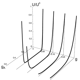
Figure 10: Scaling evolution of $U(g_{A})$ for several fixed values of $g$. This figure tracks the irrelevance/relevance of the coupling $U$ associated with the same-sublattice interaction $\bar{\rho}^{2}+\rho^{2}$ as we renormalize to stronger vector potential disorder $g_{A}~{}\rightarrow~{}\infty$, or equivalently, smaller energies $\omega~{}\rightarrow~{}0$. $U$ is normalized relative to its the bare value $U^{\,0}$ at reference energy scale $\Omega$, and we have tuned $g_{A}^{\,0}~{}=~{}0$. The non-interacting, critically delocalized phase resides at $\omega~{}=~{}0$ with $g_{A}~{}=~{}\infty$. Initially irrelevant near the clean Dirac fixed point ($g_{A}~{}\ll~{}1$), $U$ ultimately flows off to strong coupling at larger $g_{A}$, taking the model away from the non-interacting, zero energy delocalized phase.

Figure 10 shows the RG evolution of the same-sublattice interaction strength $U$ with increasing length scale as a function of the running random vector potential variance $g_{A}$ for several different values of the fixed random mass variance $g$ [see Eq. (77) below]. This plot describes the following situation: we turn on an infinitesimally small interaction strength $U^{\,0}$ and set the bare vector potential disorder $g_{A}^{\,0}=0$ at energy $\omega=\Omega$. For small $g$ this places us near the clean Dirac fixed point. Then we run the RG, flowing to smaller energies $\omega\rightarrow 0$ and stronger disorder $g_{A}\rightarrow\infty$, and we observe the evolution of the coupling $U$. When the dynamic scaling behavior crosses over from Eq. (71) to Eq. (74), this interaction strength begins to diverge strongly. The analytical expression plotted in Fig. 10 is given by

$$U(g_{A})\sim\exp\left[\frac{3}{2g^{2}}g_{A}^{2}-\left(\frac{3}{g}+\frac{1}{2g^{2}}\right)g_{A}\right].$$ (77)

Equation (77) may be obtained by combining Eqs. (IV.1), (69), and (70), setting $g_{A}^{\,0}=0$. The value of $g_{A}\equiv g_{A}^{\,U}$ where $U$ becomes relevant varies with $g$: for smaller values of $g$, the crossover occurs at smaller values of $g_{A}^{\,U}$. From Eq. (77), we have

$$g_{A}^{\,U}=\frac{1}{6}+g.$$ (78)

Note, however, that the transition at small $g$ occurs at much lower energies [since we need $g^{2}\left|\ln(\omega/\Omega)\right|$ to grow from zero ($\omega=\Omega$) to order one ($\omega\sim\Omega\exp(-1/g^{2})\ll\Omega$)]. The freezing transition in the dynamic scaling behavior is supposed to occurMRF at $g_{A}^{\,c}\sim 1+\mathcal{O}(g)$ for small $g$; Eq. (78) suggests that for $g\ll 1$, the interaction $U$ becomes relevant for $g_{A}$ well below $g_{A}^{\,c}$, potentially preventing the RG from ever reaching the non-interacting freezing transition.

The instability to interaction effects that we observe here is perhaps not so surprising when one considers the strongly-divergent form of the low-energy density of states in this “intermediate” disorder regime given by Eq. (2). The exponent is $\alpha=1/2$ in this equation. We have a picture of a large number of exotic, multifractal states crammed into a very narrow energy window; we might therefore expect that turning on interparticle interactions should produce a very strong effect. The obvious question, then, is why does the same instability not occur for weak interactions in the corresponding 1D problem?

The non-interacting disordered fermion problem with chiral symmetry [Eq.(1)] in one dimension may be formulated as random spin 1/2 quantum $XY$ chain.SachdevBook This random $XY$ chain is asymptotically solvable by a strong randomness RG procedure,DSF ; MDH1D wherein the spins connected by the strongest random bonds are systematically decimated out of the chain, replaced by ever weaker bonds connecting the surviving spins. The infrared limit of this RG is the so-called random singlet phaseDSF , which is similarBOUCHAUD , in some respects, to the non-interacting version of the 2D model considered in this paper. The addition of weak, homogeneous, short-ranged Ising $S_{i}^{z}S_{j}^{z}$ couplings to the random $XY$ spin chain, corresponding to density-density interactions in the fermion model, does not destabilize this disordered phase; in the strong randomness RG, these additional Ising bonds become ever weaker as spins coupled with strong $XY$ bonds are removed from the chain. Although some progressMDH2D has been made in applying these ideas to the non-interacting 2D chiral Dirac theory, we do not know whether this methodology may shed further light on the instability to same-sublattice interaction effects that we have found in this paper. Presumably, the higher degree of connectedness in the 2D model changes the way that the interactions are renormalized relative to the 1D case.

Recall that Eq. (75) only gives the scaling behavior of the interaction $\bar{\rho}^{2}+\rho^{2}$ (in the intermediately-disordered regime); in Eqs. (62-64), we have not written explicitly the one-loop renormalization effects of $U$ upon the disorders strengths $g$ and $g_{A}$ or the autorenormalization effects of $U$ upon itself. Although we will omit the details here, we have performed the complete one-loop RG calculation and found that all of these corrections vanish to one loop. (This eliminates the possibility of finding a new, interacting critical fixed point to lowest order in $U$.) We also know that $U$ cannot renormalize $h$ at one loop, as discussed in the paragraph below Eq. (40) in Sec. III, and thus cannot influence the dynamic scaling behavior given by Eq. (69).

The scaling equations (75) and (76) derived above apply equally to the sublattice hopping model on the square lattice with $\pi$-flux model per plaquette and real random bond disorder.HWK (The random Hamiltonian is again invariant under both chiral and time-reversal symmetries.) The operators $\bar{\rho}$ and $\rho$ have the same interpretations as local sublattice density operators because their definition [Eq. (12)] relies only upon the definition of the chiral symmetry in the continuum Dirac theory, given by Eq. (8). The sublattices of the bipartite square lattice are themselves bipartite square lattices, and next-nearest-neighbor interactions tend to produce charge-ordering on one sublattice for $U<0$, and charge stripes for $U>0$.

IV.1.3 Strong disorder: $g_{A}\gg g_{A}^{\,c}$

We can imagine that the RG flow reaches successfully the regime above the freezing transition $g_{A}>g_{A}^{\,c}$ before $U$ grows large enough to invalidate our scaling analysis, say by tuning the initial interaction strength very small. The ultimate dynamic scaling behavior at asymptotically low energies is different from that of Eq. (69); instead, for $g_{A}>g_{A}^{\,c}$, the relationship between the RG scale $l\rightarrow\infty$ and the bare energy scale $\omega\rightarrow 0$ is given byMDH2D ; MRF

$$l\sim\left(\frac{1}{c(g)}\left|\ln\frac{\omega}{\Omega}\right|\right)^{\frac{2}{3}},$$ (79)

with $c(g)\propto g+\mathcal{O}(g^{2})$. Using the same logic as above, this leads to the scaling behaviors

$$U\sim\frac{\omega}{\Omega}\exp\left[8g^{2}\left(\frac{1}{c(g)}\left|\ln\frac{\omega}{\Omega}\right|\right)^{\frac{4}{3}}\right]$$ (80)

and

$$W\sim\frac{\omega}{\Omega}\exp\left[4g\left(\frac{1}{c(g)}\left|\ln\frac{\omega}{\Omega}\right|\right)^{\frac{2}{3}}\right].$$ (81)

Equation (80) is another primary result of our paper.

The main point that we want to stress is that Eq. (80) shows that $U$ is ultimately even more relevant beyond the freezing transition, so that regardless of whether RG takes us into the regime above the freezing transition before $U$ diverges, we always find that the non-interacting description is unstable to the same-sublattice interaction effects characterized by the operator $\bar{\rho}^{2}+\rho^{2}$. We are able to extend our analysis to this large $g_{A}$ regime because the key results leading to Eqs. (80) and (81) can be obtained from the $(2+0)$D theory non-perturbatively in $g_{A}$: as discussed above Eqs. (IV.1) and (IV.1), the 1-loop flow equations for the disorder couplings $g$ and $g_{A}$ [Eqs. (62) and (63)], and for the interaction scaling dimensions [Eq. (64)] contain the exact $g_{A}$-dependence (to all orders in $g_{A}$), and we combine these results with the non-perturbative dynamic scaling relation beyond the freezing transition [Eq. (79), taken from Ref. MRF, ]. This leads to Eqs. (80) and (81).

IV.2 Summary and outlook

Within the context of our perturbative one-loop renormalization group calculation, we have found that same-sublattice interactions become strongly enhanced as one examines the TRI random chiral symmetric Dirac model at ever lower energy scales, or equivalently, larger values of the running disorder coupling $g_{A}$. We emphasized that while the calculation presented in this paper appears perturbative in both of the disorder strengths $g$ and $g_{A}$, we can extend our results to arbitrarily large values of $g_{A}$ because of the knownGLL ; MRF non-perturbative structure of the non-interacting (nearly conformal) disordered Dirac theory.

The validity of our stability analysis is restricted to $g\ll 1$; because $g$ does not evolve under the RG in the non-interacting phase, we can tune $g$ as small as we wish.

The same mechanism responsible for the instability to interaction effects drives the divergence of the density of states, and ultimately the freezing transition, in the non-interacting model. We have shown that this instability occurs regardless of whether we reach the regime beyond the freezing transition or not.

To lowest order in the interaction strength, we see no signs of the possibility of a new, interacting critical fixed point. We therefore anticipate that the strongly relevant same-sublattice interactions drive the disordered honeycomb model toward some kind of Mott insulating phase. We pointed out that the same picture obtains for the square lattice $\pi$-flux modelHWK . In the introduction we dubbed the observed evolution of the clean but interacting Dirac fixed point, weakly perturbed by chiral-symmetric disorder $g$ at some finite energy scale $\omega=\Omega$, toward a Mott insulating ground state in the limit of zero energy $\omega\rightarrow 0$, a “disorder-driven Mott transition.” In the limit of small $g$, this instability occurs only at very small energies; the scale at which the same-sublattice interactions become relevant occurs below the freezing transition for small $g$, and is roughly the same scale at which the density of states begins to diverge, as in Eq. (2) with $\alpha=1/2$.

An obvious extension of the present work would be to try to approach the interaction effects beyond the regime linear in the strengths of the interactions; indeed, the calculation presented in this paper treats the interactions only to lowest order, addressing only the question of the stability of the non-interacting description to the inclusion of interactions. The natural framework for such an extended investigation is the generalized Finkel’stein NL$\sigma$MBK , which grafts many-particle interactions from the disordered fermion theory directly into Wegner’s low energy effective theory of interacting diffusion modes. An advantage of the Finkel’stein NL$\sigma$M is that the perturbative RG is an expansion only in the dimensionless DC resistance; therefore, at least formally, even a one-loop calculation treats the interaction couplings to all orders. A calculation along these lines is currently in progressNewWork .

- (1) M. R. Zirnbauer, J. Math. Phys. 37, 4986 (1996).
- (2) A. Altland and M. R. Zirnbauer, Phys. Rev. B 55, 1142 (1997).
- (3) T. Senthil, M. P. A. Fisher, L. Balents, and C. Nayak, Phys. Rev. Lett. 81, 4704 (1998).
- (4) V. Kagalovsky, B. Horovitz, Y. Avishai, J. T. Chalker, Phys. Rev. Lett. 82, 3516 (1999); T. Senthil, J. B. Marston, and M. P. A. Fisher, Phys. Rev. B 60, 4245 (1999); I. A. Gruzberg, A. W. W. Ludwig, and N. Read, Phys. Rev. Lett. 82, 4524 (1999); E. J. Beamond, J. Cardy, and J. T. Chalker, Phys. Rev. B 65, 214301 (2002).
- (5) T. Senthil and M. P. A. Fisher, Phys. Rev. B 61, 9690 (2000).
- (6) M. Bocquet, D. Serban, and M. R. Zirnbauer, Nucl. Phys. B 578, 628 (2000).
- (7) S. Vishveshwara, T. Senthil, and M. P. A. Fisher, Phys. Rev. B 61, 6966 (2000).
- (8) N. Read and A. W. W. Ludwig, Phys. Rev. B 63, 024404 (2001).
- (9) J. T. Chalker et al., Phys. Rev. B 65, 012506 (2002).
- (10) R. Gade and F. Wegner, Nucl. Phys. B 360, 213 (1991); R. Gade, Nucl. Phys. B 398, 499 (1993).
- (11) Y. Hatsugai, X.-G. Wen, and M. Kohmoto, Phys. Rev. B 56, 1061 (1997).
- (12) M. Fabrizio and C. Castellani, Nucl. Phys. B 583, 542 (2000).
- (13) S. Guruswamy, A. LeClair, and A. W. W. Ludwig, Nucl. Phys. B 583, 475 (2000).
- (14) O. Motrunich, K. Damle, and D. A. Huse, Phys. Rev. B 65, 064206 (2002).
- (15) C. Mudry, S. Ryu, and A. Furusaki, Phys. Rev. B 67, 064202 (2003).
- (16) D. S. Fisher, Phys. Rev. B 50, 3799 (1994).
- (17) For a review, see e.g. D. Belitz and T. R. Kirkpatrick, Rev. Mod. Phys. 66, 261 (1994).
- (18) For a recent account see: S. V. Kravchenko and M. P. Sarachik, Metal-insulator transition in two-dimensional electron systems, Rep. Prog. Phys. 67, 1 (2004); A. Punnoose and A. M. Finkel’stein, Science 310, 289 (2005).
- (19) M. P. A. Fisher and E. Fradkin, Nucl. Phys. B 251, 457 (1985); E. Fradkin, Phys. Rev. B 33, 3257 (1986).
- (20) A. W. W. Ludwig, M. P. A. Fisher, R. Shankar, and G. Grinstein, Phys. Rev. B 50, 7526 (1994).
- (21) F. Wegner, Nucl. Phys. B 280, 210 (1987).
- (22) A. D. Mirlin, Phys. Rep. 326, 259 (2000).
- (23) F. Evers, A. Mildenberger, and A. D. Mirlin, Phys. Rev. B 64, 241303(R) (2001).
- (24) C. C. Chamon, C. Mudry, and X.-G. Wen, Phys. Rev. Lett. 77, 4194 (1996).
- (25) H. E. Castillo, C. C. Chamon, E. Fradkin, P. M. Goldbart, and C. Mudry, Phys. Rev. B 56, 10668 (1997).
- (26) O. Motrunich, K. Damle, and D. A. Huse, Phys. Rev. B 63, 134424 (2001).
- (27) See e.g. J. P. Bouchaud, A. Comtet, A. Georges, and P. Le Doussal, Ann. Phys. (N.Y.) 201, 285 (1990); L. Balents and M. P. A. Fisher, Phys. Rev. B 56, 12970 (1997); M. Bocquet, Nucl. Phys. B 546, 621 (1999).
- (28) P. Fendley and R. M. Konik, Phys. Rev. B 62, 9359 (2000).
- (29) P. A. Lee and D. S. Fisher, Phys. Rev. Lett. 47, 882 (1981).
- (30) A. Furusaki, Phys. Rev. Lett. 82, 604 (1998).
- (31) S. Ryu and Y. Hatsugai, Phys. Rev. B 65, 033301 (2002).
- (32) M. Bocquet and J. T. Chalker, Phys. Rev. B 67, 054204 (2003); Ann. Henri Poincaré 4, S539 (2003).
- (33) Recent numerical work (excluding interactions) for a certain special kind of disorder was presented in V. M. Pereira et al., Phys. Rev. Lett. 96, 036801 (2006).
- (34) D. Bernard, (Perturbed) conformal field theory applied to 2d disordered systems: an introduction, in: Cargèse lectures, NATO Science Series: Physics B, vol. 362 (1997), L. Banlieu et al. (eds.); hep-th/9509137.
- (35) C. Mudry, C. Chamon and X.-G. Wen, Nucl. Phys. B 466, 383 (1996).
- (36) D. Carpentier and P. Le Doussal, Phys. Rev. Lett. 81, 2558 (1998); Nucl. Phys. B 588, 565 (2000).
- (37) M. L. Horbach and G. Schoen, Ann. Phys. (Leipzig) 2, 51 (1993); A. Kamenev and A. Andreev, Phys. Rev. B 60, 2218 (1999); C. Chamon, A. W. W. Ludwig, and C. Nayak, Phys. Rev. B 60, 2239 (1999).
- (38) See e.g. D. J. Amit, Field Theory, the Renormalization Group, and Critical Phenomena, 2nd ed. (World Scientific, Singapore, 1984).
- (39) See e.g. S. Sachdev, Quantum Phase Transitions (Cambridge University Press, New York, 2000).
- (40) M. S. Foster and A. W. W. Ludwig (unpublished).