An orbital-free self-consistent field approach for molecular clusters and liquids

Abstract

We present an “orbital” free density functional theory for computing the quantum ground state of atomic clusters and liquids. Our approach combines the Bohm hydrodynamical description of quantum mechanics with an information theoretical approach to determine an optimal quantum density function in terms of density approximates to a statistical sample. The ideas of Bayesian statistical analysis and an expectation-maximization procedure are combined to develop approximations to the quantum density and thus find the approximate quantum force. The quantum force is then combined with a Lennard-Jones force to simulate clusters of Argon atoms and to obtain the ground state configurations and energies. As demonstration of the utility and flexibility of the approach, we compute the lowest energy structures for small rare-glass clusters. Extensions to many atom systems is straightforward.

I Introduction

It has been long recognized that computational effort of grid-based quantum mechanical methods for nuclear dynamical problems grows exponentially with the number of degrees of freedom. This limits the size of systems that can be handled in an exact manner to those with 4 or less atoms. This is perhaps best illustrated in the field of reactive scattering experiments which have been limited to systems with 6D Zhang and Zhang (1994); Zhang and Light (1996); Somers et al. (2004); Echave and Clary (1994), but it is also clearly seen in other areas such as photodissociation processes. Guo et al. (1991); Manth and Koppel (1991) In light of this, considerable progress has been made in developing rigorous approaches for contracting the basis size required to perform such calculations. One such approach that has seen considerable success is the multi-configurational time-dependent Hartree approach (MCTDH) developed by Meyer and co-workersManthe et al. (1990, 1992) that overcomes this limitation in a numerically exact way by expanding the time-dependent wave function in terms of a number of time-dependent configurations.

$$\Psi(t)=\sum_{J}A_{J}(t)\Phi_{J}(t),$$

in which the single particle (or quasi-particle) basis functions $\Phi_{J}(t)$ and the expansion coefficients are are coupled by the MCTDH equations of motion.

For condensed phase systems and liquids path integral Monte Carlo (PIMC) and centroid based molecular dyamics remain the method of choice. They have been extremely successful in calculating a wide variety of different thermodynamic properties of heavily quantum systems. Calvo et al. (2001); Rick et al. (1991); Neirotti et al. (2000); Chakravarty (1995a) Despite the success of PIMC approaches of late there are some inherent difficulties it faces. For instance, at low temperatures the amount of parameters that must be included can become prohibitive and lead to slow convergence.

We present an approach which can model low temperature Lennard-Jones clusters with ease. The method developed herein develops along analogous lines to the MCTDH approach and can be best thought of as an “orbital” free approach since we work entirely at the level of the nuclear $N$-body density. We do this by first writing the configurational density $n(1\cdots N)$ that describes the statistical likelihood of finding the system in a given multi-dimensional configuration $\{r_{1}\cdots r_{N}\}$ as a superposition of statistical approximates $p(r_{1}\cdots r_{N},c_{m})$ that are joint probabilities for finding system at $\{r_{1}\cdots r_{N}\}$ and that it is a variant of some statistical distribution described by the approximate. These approximates can be any elementary probability distribution function that can be specified in terms of its statistical moments, $c_{m}$, the simplest of which for our purposes are multi-dimensional gaussians. In this case, we need to be able to specify $m(3N(3N+1)/2+3N+1)={\cal O}(mN^{2})$ variables corresponding to the elements of the covariance matrix, the central mean, and amplitude for $m$ $3N$-dimensional gaussians.

Explicit correlations between various degrees of freedom can be excluded in straightforward way by factoring the approximates. For example, if we factorize the full covariance matrix into individual atomic components, the configurational density can be cast in terms of the individual atomic densities

$$n(1\cdots N)=\prod_{i=1}^{N}n_{i}(r_{i}).$$ (1)

We can then expand each atomic density $n_{i}(i)$ as a linear combination of density approximates.

$$n_{i}(r_{i})=\sum_{m=1}^{M}p_{mi}(c_{mi},r_{i}),$$ (2)

This dramatically reduces the number of coefficients we need to determine to $mN\times(6+3+1)={\cal O}(mN)$. Intermediate factorization scheme yield similar scaling behavior allowing one to tune the computational complexity of the system depending upon the degree of correlation required by a particular physical problem. For example, one can define quasi-atoms by explicitly including covariance between the degrees of freedom of 2 or more atoms. As we shall derive next, each quasi-atom or atom will then evolve in the mean-field of the other quasi-atoms of the system.

In this paper, we present a grid-free adaptive hydrodynamic approach for computing the quantum ground-state density for a system of $N$ nuclei. Our approach uses Bayesian analysis to deduce from a statistical sampling of the density the best set of $m$ statistical approximates describing that density. We then use a quantum hydrodynamical scheme to move the sample points towards a minimal energy configuration. As proof of concept we consider the zero-point energy of small 4 and 5 atom clusters of Argon and Neon with pair-wise interatomic potential interactions. Finally, we discuss how the approach may be used to develop new quantum-classical and fully quantum mechanical approaches for treating quantum mechanical solute particles (such as an excess e^- or He atom) in a liquid of classical or quasi-classical atoms (such as Ar or Ne).

II Self-consistent field equations

We begin by writing the full many-body Hamiltonian for the nuclear motion of a collection of atoms with pair-wise interaction potentials.

$$H=-\sum_{i=1}^{N}\frac{1}{2m_{i}}\nabla_{i}^{2}+\sum_{i\neq j}V(ij),$$ (3)

where the first is the sum of the kinetic energies of the individual atoms and the second is the sum of the potential energy contributions. For an arbitrary $N$-body trial density, the energy functional is given by

$$E[n]=T[n]+\sum_{i\neq j}\int\int n_{i}(r_{i})n_{j}(r_{j})V(ij)dr_{i}dr_{j}.$$ (4)

Since the kinetic energy operator is separable and we have assumed distinguishability amongst the constituent atoms, the kinetic energy term is the sum of the individual kinetic energy functionals.

$$T[n(1\cdots N)]=\sum_{i=1}^{N}T_{i}[n(r_{i})],$$ (5)

As in electronic structure DFT, evaluating the kinetic energy functionals in an orbital free form is problematic since evaluating the quantum kinetic energy operator is a non-local operator and the density is a local function. Parr and Yang (1989),

If instead we write the quantum wave function in polar form, as in the hydrodynamic formulation of quantum mechanicsMadelung (1926); de Broglie (1926, 1927),

$$\Psi(1\cdots N)=\sqrt{n(1\cdots N)}e^{i\phi(1\cdots N)},$$ (6)

we can arrive at a stationary condition that if $\vec{\nabla}\phi=0$Holland (1993),

$$V(1\cdots N)-\sum_{i}\frac{1}{2m_{i}}\frac{1}{\sqrt{n(r_{i})}}\nabla_{i}^{2}\sqrt{n(r_{i})}=const,$$ (7)

at all points in space. The constant is of course the energy. By inspection, then, we can define our kinetic energy functional as

$$T[n(r_{i})]=-\frac{1}{2m_{i}}\int\sqrt{n(r_{i})}\nabla_{i}^{2}\sqrt{n(r_{i})}dr_{i}.$$ (8)

Integrating by parts and letting $n(i)\rightarrow 0$ at $\pm\infty$ produces the familiar von Weizsacker kinetic energy functionalvon Weizsacker (1935)

$$T_{W}[n(r_{i})]=+\frac{1}{8m}\int\frac{1}{n(r_{i})}\vec{\nabla}_{i}n(r_{i})\cdot\vec{\nabla}_{i}n(r_{i})dr_{i}.$$ (9)

Thus, the total energy functional is given in terms of the single particle densities.

$$E[n]=\sum_{i=1}^{N}T_{W}[n_{i}(r_{i})]+\sum_{i\neq j}\int\int n_{i}(r_{i})n_{i}(r_{j})V(ij)dr_{i}dr_{j}.$$ (10)

Taking the variation of $E[n]$ with respect to the single-particle densities with the constraint that $\sum_{i}\int n_{i}(r_{i})di=N$,

$$\delta\left\{\sum_{i=1}^{N}\left(T_{W}[n_{i}(r_{i})]+\sum_{j\neq i}\int\int n_{i}(r_{i})n_{j}(r_{j})V(ij)dr_{i}dr_{j}-\mu\left(\int n_{i}(r_{i})dr_{i}-1\right)\right)\right\}=0,$$ (11)

leads to the following Euler-Lagrange equations:

$$\frac{\delta T_{W}[n_{i}(r_{i})]}{\delta n_{i}(r_{i})}+\sum_{j\neq i}\int V(ij)n_{j}(r_{j})dr_{j}-\mu=0.$$ (12)

When satisfied, $\mu$ is the vibrational ground-state energy and the $n_{i}(r_{i})=|\phi_{i}(i)|^{2}$ are the probability densities of the individual nuclei.

Let us take a simple pedagogic case of a particle in a harmonic well, taking the trial density density to be a Gaussian, $n(x)=\sqrt{a/\pi}\exp(-ax^{2})$. Evaluating the energy functional yields:

$$E[n(x)]=\frac{1}{4m}a+\frac{m\omega^{2}}{4a}.$$

Minimizing with respect to the trial density

$$\frac{\delta E[n]}{\delta n}=\frac{dE}{da}=0,$$

yields the familiar $E=\omega/2$ and $a=m\omega$. This idea is easy to extend beyond purely harmonic systems and gaussian trial functions. Since $n(i)$ is a probability distribution function, it is a positive, real, and integrable function.

In the next section, we show how the single particle densities can be estimated as super-positions of single particle density approximates and that the coefficients (rather moments) of the approximates can be optimized to compute both the ground state energy and the single-particle densities.

III Mixture Modeling

The single-particle probability distribution functions (PDF) can be represented by a mixture model Gershenfeld (1999); McLachlan and Basford (1998) by summing a finite number $M$ of density approximates

$$n(r)=\sum_{m}^{M}p({\bf r},c_{m}),$$ (13)

where $p({\bf r},cm)$ is the probability that a randomly chosen member of the ensemble has the configuration ${\bf r}$ and is a variant of the $m$th approximate designated by $c_{m}$. These approximates may be Gaussians or any other integrable multi-dimensional function which can be parameterized by its moments. For gaussian clusters, we have a weight $p(c_{m})$, a mean position vector $\mu_{m}$, and a covariance matrix $C_{m}$.

By definition, each joint probability in Eq. 13 is related to a pair of conditional probabilities according to the relation

$$p({\bf r},c_{m})=p(c_{m})p({\bf r}|c_{m})=n({\bf r})p(c_{m}|{\bf r}),$$ (14)

where the forward conditional probability $p({\bf r}|c_{m})$ refers to the probability that a randomly chosen variant of $c_{m}$ has the configuration $r$. Conversely, the posterior probability $p(c_{m}|{\bf r})$ refers to the probability that the configuration point $r$ is a variant of the approximate $c_{m}$. In probability theory, $n(r)$ and $p(c_{m})$ are known as marginal probabilities; however, we shall simply refer to them as the quantum density and weight of the $m$th approximate, respectively. The expansion weights are strictly positive semidefinite and sum to unity. Substituting the first equality of Eq. 14 into Eq. 13 we have

$$n({\bf r})=\sum_{m}^{M}p(c_{m})p({\bf r}|c_{m}).$$ (15)

We have considerable freedom at this point in specifying the exact functional form of the conditional probabilities as well as the degree of correlation within each conditional. This freedom of specification allows us to construct “models” that explicitly take into account nonseparable correlations in configuration space. For the case of gaussian approximates this is accomplished by keeping or discarding various off-diagonal terms incorporates in the covariance matrix, C,

$$p({\bf r}|c_{m})=\sqrt{\frac{\|{\bf C}^{-1}\|}{(2\pi)^{N_{d}}}}e^{({\bf r}_{d}-\mu_{m,d}).\bf{C}_{m}^{-1}.({\bf r}_{d}-\mu_{m,d})}.$$ (16)

The term,$\|{\bf C}^{-1}\|$, stands for the reciprocal of the greatest value of the determinant of the covariance matrix. It is also possible to construct a model that assumes that each approximate is completely separable and takes the form of a product over the $N_{d}$-dimensional configuration space, that reduces the covariance matrix, $\bf{C}$, to a variance vector,

$$p({\bf r}|c_{m})=\prod_{d}^{N_{d}}\sqrt{\frac{1}{2\pi\sigma_{m,d}^{2}}}\exp(({\bf r}_{d}-\mu_{m,d})^{2}/(2\sigma_{m,d}^{2})).$$ (17)

Numerical tests by Maddox and Bittner indicate that separable case is computationally faster for high dimensional systems, but produces a less accurate estimate of the quantum ground-state energy. Maddox and Bittner (2003) For larger systems the noncovariant case can certianly be used to speed calculations. We will examine the case where there is nonzero covariance between the three dimensions, but the atomic degrees of freedom have zero overlap. For a discussion of the strengths and weaknesses involved with mixture models, one is referred to the Refs. Maddox and Bittner (2003); Heller (1981). This approximation provides a sufficient approximation to the density for the calculation of the ground state.

Once a model is decided upon one must then determine the parameters, in this case the Gaussian parameters $p(c_{m})$, $\mu_{m}$, and $C_{m}$, for each approximate from the statistical points representing the density. For instance the mean position vectors of the approximates are defined by the moments of the forward conditional probabilities

$${\bf\mu}_{m}=\int{\bf r}p({\bf r}|c_{m})d{\bf r}.$$ (18)

Rearranging Eq. 14 and substituting into Eq. 18, we can write these parameters as

$${\bf\mu}_{m}=\int{\bf r}\frac{n({\bf r})p(c_{m}|{\bf r})}{p(c_{m})}d{\bf r},$$ (19)

this is easily approximated by summing over an ensemble of points $\{{\bf r}_{n}\}$ sampled from the $n(r)$ PDF,

$${\bf\mu}_{m}\approx\frac{1}{Np(c_{m})}\sum_{n}^{N}{\bf r}_{n}p(c_{m}|{\bf r}_{n}).$$ (20)

We also define similar expressions for the covariance matrix and the expansion weights

$$p(c_{m})\approx\frac{1}{N}\sum_{n}^{N}p(c_{m}|{\bf r}_{n}),$$ (21)

$${\bf C}_{m}\approx\frac{1}{Np(c_{m})}\sum_{n}^{N}({\bf r}_{n}-{\bf\mu})^{T}({\bf r}_{n}-{\bf\mu})p(c_{m}|{\bf r}_{n}).$$ (22)

For the separable case, the variances are given by the diagonal elements $\sigma_{m,i}^{2}=(C_{m})_{ii}$. The posterior terms $p(c_{m}|{\bf r}_{n})$ for each ${\bf r}_{n}$ sample point in Eqs. 20-22 are evaluated directly from the forward probabilities according to Bayes’ equation,

$$p(c_{m}|{\bf r}_{n})=\frac{p(c_{m})p({\bf r}_{n}|c_{m})}{\sum_{m}p(c_{m})p({\bf r}_{n}|c_{m})}.$$ (23)

Within this viewpoint, the sample points can be considered to be a data set that represents the results of a series of successive measurements. Each data point carries an equal amount of information describing the underlying quantum probability distribution function. Bayes’ equation gives the ratio of how well a given estimate describes ${\bf r}_{n}$ to how well ${\bf r}_{n}$ is described by all of the approximates. Thus, it represents the fraction of explanatory information that a given sample point gives to the $m$-th approximate. The estimate which best describes the point will have the largest posterior probability at that point. Eqs. 20-23 can be iterated self-consistently in order to determine the best possible set of parameters that describe $n(r)$ in terms of a given ensemble of data points. In doing so, we effectively maximize the log-likelihood that the overall density model describes the entire collection of data points.

$$L=\log\prod_{n}n({\bf r}_{n}),$$

Taking the variation of $L$ with respect to the model parameters generates a series of update-rules for moving the approximates through parameter space in the direction along $\vec{\nabla}_{c_{m}}L$.Gershenfeld (1999). For the case of Gaussian approximates, the update rules for the mean, covariance matrix, and marginal probabilities are given by,

$$\delta\mu_{m}=\frac{{\bf C}_{m}}{Np(c_{m})}\vec{\nabla}_{\mu_{m}}L,$$

$$\delta{\bf C}_{m}=\frac{2({\bf C}_{m}\otimes{\bf C}_{m})}{Np(c_{m})}\vec{\nabla}_{{\bf C}_{m}}L,$$

$$\delta p(c_{m})=\frac{1}{N}({\rm diag}[\Omega]-\Omega(\Omega)^{T})\vec{\nabla}_{p(c_{m})}L.$$

Where $\otimes$ is the Kronecker product, $\Omega$ is the vector of all expansion weights, $\Omega=[p(c_{1}),\ldots,p(c_{m})]^{T}$, and ${\rm diag}[\Omega]$ is a matrix with the elements from $\Omega$ constituting the diagonal entries. Xu and Jordan (1996)

The expectation maximization algorithm described above allows us to generate an approximate analytical functional form for the single particle density via statistical sampling over an ensemble of points. The next step is to adjust the single-particle densities themselves to produce a lower total energy. We do this by deriving the quantum hydrodynamic equations of motion for the sample points. The quantum Hamilton-Jacobi equation generates the equations of motion for the ray-lines of a time-dependent solution to the Schrödinger equation.Bohm (1952a, b); Bohm et al. (19878); Wyatt (1999).

$$\frac{\partial S}{\partial t}+\sum_{i}\frac{|\vec{\nabla}_{i}S|^{2}}{2m_{i}}+\sum_{i\neq j}\int\int n_{i}(r_{i})n_{j}(r_{j})V(ij)dr_{i}dr_{j}-\sum_{i}\frac{1}{2m_{i}}\frac{1}{\sqrt{n_{i}(r_{i})}}\nabla_{i}^{2}\sqrt{n_{i}(r_{i})}=0$$ (24)

Since the density is separable into components, we easily arrive at a set of time-dependent self-consistent field equations whereby the motion of atom $i$ is determined by the average potential interaction between atom $i$ and the rest of the atoms in the system.

$$\dot{S}(i) + \frac{|\vec{\nabla}_{i}S|^{2}}{2m_{i}}+\sum_{j\neq i}\int V(ij)n_{j}(r_{j})dr_{j}$$ (25)

$$- \frac{1}{2m_{i}}\frac{1}{\sqrt{n_{i}(r_{i})}}\nabla_{i}^{2}\sqrt{n_{i}(r_{i})}=0.$$

Taking $\vec{\nabla}S={\bf p}=m_{i}\dot{\bf r}$ as a momentum of a particle, the equations of motion along a given ray-line or characteristic ${\bf r_{n}}(t)$ of the quantum wave function are given by

$$m_{i}\ddot{\bf r}_{n}=-\sum_{j\neq i}\int(\vec{\nabla}_{i}V(ij))n_{j}(r_{j})dr_{j}-\vec{\nabla}_{i}Q[n_{i}(r_{i})]$$ (26)

where $Q[n(i)]$ is the Bohmian quantum potential specified by the last term in Eq. 25. Stationary solutions of time-dependent Schrödinger equation are obtained whenever $m_{i}\ddot{\bf r}_{n}=0$. Consequently, by relaxing the sample points in a direction along the energy gradient specified by

$$\vec{\nabla}_{i}E=-\sum_{j\neq i}\int(\vec{\nabla}_{i}V(ij))n_{j}(r_{j})dr_{j}-\vec{\nabla}_{i}Q[n_{i}(r_{i})].$$ (27)

keeping $n(r_{j})$ fixed. This generates a new statistical sampling, which we then use to determine a new set approximates.

This process is similar to the semiclassical approximation strategy for including quantum effects into otherwise classical calculations introduced by Garaschuk and Rassolov Garashchuk and Rassolov (2003, 2002). This semiclassical approximate methodology is based upon de Broglie-Bohm trajectories and involves the convolution of the quantum density with a minimum uncertainty wave packet which is then expanded in a linear combination of Gaussian functions

$$\rho(x)\approx f(x)=\sum_{n}c_{n}^{2}\exp[-a_{n}^{2}(x-X_{n})].$$ (28)

The Gaussian parameters $s=\{c_{n},X_{n},a_{n}\}$ in Eq. 28 are determined by minimizing the functional

$$F=\int[\rho(x)-f(x)]^{2}dx$$ (29)

using an iterative procedure which explicitly involves solving the set of equations $\partial F/\partial s_{k}=0$. The parametrized density leads to an approximate quantum potential (AQP) that is used to propagate an ensemble of trajectories. This approach has been used successfully in computing reactive scattering cross-sections for the co-linear H+H₂ reaction in one dimension.

It is important at this point to recognize the numerical difficulties our group and others have faced in developing hydrodynamic trajectory based approaches for time-dependent systems. Lopreore and Wyatt (1999); Wyatt (1999); Kendrick (2003); Maddox and Bittner (2003); Wyatt and Bittner (2000); Hughes and Wyatt (2002) The foremost difficulty is in the accurate evaluation of the quantum potential from an irregular mesh of points. Lopreore and Wyatt (1999); Wyatt and Bittner (2000) The quantum potential is a function of the local curvature of the density and can become singular and rapidly varying as nodes form in the wave function or when the wave function is sharply peaked, i.e. when $n^{1/2}\to 0$ faster than $\nabla^{2}n^{1/2}\to 0$. These inherent properties make an accurate numerical calculation of the quantum potential and its derivatives very difficult for all but the simplest systems. These difficulties are avioded in the cluster model approximation of the density, using the expectation maximization (EM) algorithm,Maddox and Bittner (2003). By obtaining a global optimal function that describes the density, we can analytically compute the quantum force with great accuracy. The issue of nodes is essentially avoided so long as we are judicious in our choice of density approximates. If we choose node-free approximates, then our overall density will likewise be node free. For the purpose of determining vibrational ground-states, this seems to be a worthwhile compromise.

The algorithm can be summarized as follows

1. For each atom, generate and sample a normalized trial density $n_{i}(r_{i})$.

2. Using the EM routines and the given sample of points, compute the coefficients for the density approximates.

3. Compute the forces on each point using Eq. 27 and advance each point along the energy gradient for one “time” step, either discarding or dampening the velocity of each point. This generates a new sample of points describing the single-particle density for each atom. The new distribution should have a lower total energy since we moved the sample points in the direction towards lower energy.

Iterating through these last two steps, we rapidly converge towards the energy minimum of the system.

IV Vibrational ground state of rare-gas clusters

As proof of concept we examine the ground vibrational state energies of Lennard-Jones clusters. The simple Lennard-Jones pair potential provides reliable information about complicated systems, and has been used in a number of recent studies with just a few examples listed in Refs. Berry (1994); Lynden-Bell and Wales (1994); Predescu et al. (2005). Ground state energies of rare gas clusters are easily enough modeled with molecular dynamics simulations, but the quantum corrections are often quite large for these cases. These corrections are important because the quantum character strongly affects the thermodynamics via changes in the ground state structure due to increasing zero-point energies Calvo et al. (2001). The zero point energy corrections for the small clusters modeled here can be up to $0.66$kJ/mole. Indeed, quantum corrections have been shown to lower solid to liquid transition temperatures by approximately $10\%$, and the zero point energy for small clusters can account for up to $35\%$ of the classical binding energy.Chakravarty (1995b).

The effects from quantum delocalization are intuitively understood in the present approach through the quantum potential term in the equations of motion. This explains why the quantum delocalization can account for a lowering of the transition temperature because some kinetic energy is always present even at very low temperatures. This spreading of the wave packet is known as a “softening” of the crystal which leads to a lowering of the melting temperature.Chakravarty (2002) These effects have been studied in the context of the transition from molecular to bulk-like properties of clusters.

In the calculations presented here, we used 300 statistical points to represent the density of each atom and propagated the SCF equations described above until the energy and the density were sufficiently converged. Typically, this required 1.5 million to 3 million cycles. Along the course of the energy minimization, we strongly damped the time-evolution of the sample points to eliminate as much of the oscillations and breathing of the density components as possible.

The Lennard-Jones parameters for the Argon clusters are $\epsilon=0.9976$ kJ/mole and $\sigma=3.42\AA$, and $\epsilon=0.3059$ kJ/mole and $\sigma=2.79\AA$ for the Neon clusters Livesly (1983). Initial configurations for the simulations are chosen to be close to the classical molecular dynamics minimum energy geometry, and are given some initial Gaussian spread.

We show in Fig. 1 isodensity (0.006) contour plots for the Ar₄, Ar₅, Ne₄, and Ne₅.. One can see quite clearly the underlying three-dimensional shape of the cluster along with the delocalization of each atom about its central location. Each density ”lobe” is nearly spherical with some elongation. These density plots give a suggestive view of the overlap of the densities which is ignored in Eq. 1 and therefor ultimately in Eq. 9. For this system this overlap turns out to be minor, but for atoms such as Helium this would have to be taken into account.

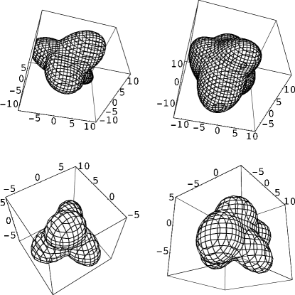
Figure 1: The isodensity contour plots of the clusters at a value of $0.006$. In the upper left is the Ar₄ cluster, in the upper right is the Ne₄, lower left has the Ar₅, and then bottom right is Ne₅. The axis are listed in atomic units.

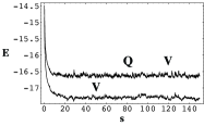
Figure 2: The average potential energy $\langle V\rangle$ and total energy $\langle Q\rangle+\langle V\rangle$ of the Ar₅ and Ne₅ clusters in kJ/mole. The steps are measured in millions.

In Fig. 2 we show the total energy an the total potential energy for the Ar₅ and Ne₅ clusters as the system converges towards its lowest energy state. Initially there is a rapid restructuring of the densities as they adjust to find a close approximation to the actual ground state density. Following this initial rapid convergence, there is slower convergence phase as the density is further refined. During this process as the sample points look for a configuration which fully equalizes of the quantum and kinetic energy terms from Eq. 7 the density approximation can sometimes prove inadequate and points can be pushed into temporary higher energy regions. This leads to the fluctuations seen in the energies and any other averaged quantity, such as the interatomic distances. In order to compute meaningful values for the energy and distances, we averaged these quantities over the last half million or so cycles. As can be seen from Figure 2 the Ne₅ cluster is slower to converge, but eventually does so around step 200(million).

Tables 1 and 2 lists the averaged interatom distances for each cluster compared to the equilibrium distances for the corresponding classical case. For the case of $Ar_{5}$ the numerical fluctuations lead to an uncertainly of about 0.3% in the interatomic distances and for $Ne_{5}$, a 0.5% uncertainty in the interatomic distances. it is important to note that the fluctuations mentioned here get smaller for larger systems as can seen by comparing the results for Ar₅ with Ar₄. This is because the well depths for the sample points become more pronounced. This has important implications since we hope to extent this method to larger systems. Ne₄ can be seen to have the largest fluctuations, which is expected since it is the most quantum mechanical. All in all these values compare well with the classical distances. In general, the quantum distances are slightly larger due to the fact that the gaussian atom densities are sampling part of the anharmonic attractive portion of the pair-potential.

Table 1: Inter-atomic distances for X₅ clusters in atomic units.

distances	Argon	Argon (cl)	Neon	Neon (cl)
$rd_{1,2}$	7.343$\pm$.019	7.225	6.167$\pm$.045	5.927
$rd_{1,3}$	7.327$\pm$.018	7.225	6.115$\pm$.031	5.927
$rd_{1,4}$	7.288$\pm$.018	7.199	6.057$\pm$.035	5.906
$rd_{1,5}$	7.269$\pm$.016	7.199	6.048$\pm$.027	5.906
$rd_{2,3}$	7.339$\pm$.023	7.225	6.162$\pm$.055	5.927
$rd_{2,4}$	7.276$\pm$.018	7.199	6.060$\pm$.039	5.906
$rd_{2,5}$	7.285$\pm$.016	7.199	6.070$\pm$.035	5.906
$rd_{3,4}$	7.266$\pm$.018	7.199	6.112$\pm$.060	5.906
$rd_{3,5}$	7.271$\pm$.016	7.199	6.077$\pm$.035	5.906
$rd_{4,5}$	11.832$\pm$.020	11.7349	9.848$\pm$.039	9.627

Table 2: Inter-atomic distances for X₄ clusters in atomic units.

distances	Argon	Argon (cl)	Neon	Neon (cl)
$rd_{1,2}$	7.362$\pm$.024	7.21	6.167$\pm$ .043	5.918
$rd_{1,3}$	7.296$\pm$.017	7.21	6.104 $\pm$ .051	5.918
$rd_{1,4}$	7.294$\pm$.019	7.21	6.092 $\pm$ .049	5.918
$rd_{2,3}$	7.320$\pm$.022	7.21	6.140 $\pm$ .038	5.918
$rd_{2,4}$	7.305$\pm$.016	7.21	6.077 $\pm$ .027	5.918
$rd_{3,4}$	7.286$\pm$.017	7.21	6.094 $\pm$ .040	5.918

Table 3 summarizes the various contributions to the the total energy for each cluster . The “classical” energies, $V_{c}$ are the energy minimum of the total potential energy surface corresponding to the classical equilibrium configuration. $\langle V\rangle$, $\langle Q\rangle$, and $\langle E\rangle$ are the total quantum potential energy, kinetic energy, and total energy of each cluster. The difference between the classical potential minimum, V_c and $\langle$E$\rangle$ is the zero point energy. For our results we calculate a virial-like term which is the ratio of the kinetic to the potential energy of the system, $\langle Q\rangle/\langle V\rangle$. It turns out the values we get for this term, seen in Table 3, are remarkably close to the values of the de Boer parameter, $\Lambda$, for the atoms we are examining.

Table 3: Table of the energies of the clusters in kJ/mole.

	Ar4	Ne4	Ar5	Ne5
$V_{c}$	-11.972	-3.655	-18.166	-5.545
$\langle V\rangle$	-11.337$\pm$.225	-3.184$\pm$ .056	-17.302 $\pm$ .344	-4.895$\pm$.055
$\langle Q\rangle$	0.462$\pm$.033	0.460 $\pm$ .034	0.669 $\pm$ .041	0.646$\pm$.036
$\langle E\rangle$	-10.874$\pm$.215	-2.724 $\pm$ .049	-16.632 $\pm$ .330	-4.249$\pm$.043
$\langle Q\rangle/\langle V\rangle$	0.041	0.144	0.038	0.132

The de Boer parameter has been used in attempts to rationalize the effects of quantum delocalization for Lennard-Jones systems. Chakravarty (1995b, a); Calvo et al. (2001) Each Lennard-Jones system can be defined in terms of its parameters $\epsilon$, or its potential depth, its length scale of $\sigma$, and mass $m$. For a given set of parameters, the thermal de Broglie wavelength, $\lambda=\hbar/\sigma\sqrt{mk_{B}T}$ provides a means of approximating the quantum effects, at some reduced temperature of the system, $T^{*}=k_{B}T/\epsilon$. Further taking the ratio of $\lambda$ for two different sets of parameters provides a means of comparing the quantum effects of one system versus the other. This leads to the de Boer parameter, $\Lambda=\hbar/r_{m}\sqrt{m\epsilon}$, which is the ratio of the de Broglie wavelength of an atom with energy $\epsilon$, with an intermolecular distance, $r_{m}$. Basically, the de Boer parameter is useful for comparing the quantum character of different Lennard-Jones clusters or liquids at a given temperature, in our case zero. M. Toda and Saito (1992) $\Lambda$ has a classical limit of $\Lambda=0$ and anything above $\Lambda\approx 0.3$ is considered a quantum system. For Argon the de Boer parameter is, $\Lambda\approx 0.03$ which corresponds to a classical system, and quantum effects can be treated as a perturbation. For Neon the de Boer parameter turns out to be $\Lambda\approx 0.1$ which is a quasi-quantum system.

The de Boer parameter measures the delocalization of the system compared to its size. The virial like term measures the percentage energy contained in the kinetic term of the Hamiltonian. The kinetic energy, also called the quantum potential energy, is also a measure of the delocalization of the system. So we see that the two terms are essentially measuring the same entity. For our results we also see a possible trend to smaller values of $\langle Q\rangle/\langle V\rangle$, as the system gets larger.

V Discussion

A method for calculating ground state configuration of quantum clusters and liquids has been outlined based upon some previous work in approximating densities as quantum statistical distribution function. The quantum and the Lennard-Jones potentials are used to propagate an ensemble of Monte Carlo statistical points, in a DFT like procedure. This is an orbital free approach in the sense that we only work at the level of the nuclear density. In order to do this we outline a “cluster” model and expectation maximization (EM) algorithm which is used to obtain the density in terms of the statistical points representing each atom. The Lennard-Jones potential is calculated in a mean field sense by averaging over the statistical points of each atom, and the quantum potential is calculated from the density obtained in the EM algorithm. Results were presented for 4 and 5 atom clusters of Argon and Neon. The results indicate good agreement with the general classical results, but the quantum corrections can be seen to be significant. Also shown is that the virial term we measure to approximate the quantum effects is related to the de Boer parameter used in previous studies.

The method outlined also seems to provide a means of artificial control of the amount of quantum mechanical information desired from a calculation. The covariances between atoms may be set to zero as we have done, which corresponds to distinguishable particles, but keeping the interatomic covariances seems to provide a possible path to including other effects such as exchange energies and the like. This all comes at the expense of increased complexity and reduced computational speed.

One could also tune the amount of quantum effects by making $\hbar$ a parameter that can vary between the values of $0$ to $1$, in atomic units, in the equation for the quantum potential. Additionally the method is easily extended to potentials beyond the Lennard-Jones. For instance, covalent bonds could be modeled with harmonic oscillators or Morse potentials, and Coulomb potentials are easily modeled.