Multicritical point of Ising spin glasses on triangular and honeycomb lattices

Abstract

The behavior of two-dimensional Ising spin glasses at the multicritical point on triangular and honeycomb lattices is investigated, with the help of finite-size scaling and conformal-invariance concepts. We use transfer-matrix methods on long strips to calculate domain-wall energies, uniform susceptibilities, and spin-spin correlation functions. Accurate estimates are provided for the location of the multicritical point on both lattices, which lend strong support to a conjecture recently advanced by Takeda, Sasamoto, and Nishimori. Correlation functions are shown to obey rather strict conformal-invariance requirements, once suitable adaptations are made to account for geometric aspects of the transfer-matrix description of triangular and honeycomb lattices. The universality class of critical behavior upon crossing the ferro-paramagnetic phase boundary is probed, with the following estimates for the associated critical indices: $\nu=1.49(2)$, $\gamma=2.71(4)$, $\eta_{1}=0.183(3)$, distinctly different from the percolation values.

I INTRODUCTION

In this paper we study two-dimensional Ising spin glasses, i.e., Ising spin–$1/2$ magnetic moments interacting via nearest-neighbor bonds $J_{ij}$ of the same strength and random sign, drawn from a quenched probability distribution:

$$P(J_{ij})=p\,\delta(J_{ij}-J_{0})+(1-p)\,\delta(J_{ij}+J_{0})\ .$$ (1)

Our interest focuses on the region of high (low) concentration $p$ ($1-p$) of ferro- (antiferro-)magnetic bonds, where even in two dimensions one can have order at $T\neq 0$. A critical line on the $T-p$ plane separates paramagnetic and ferromagnetic phases. Furthermore, for general space dimensionality $d\geq 2$ there is a second line of interest on the $T-p$ plane, along which several exact results have been derived, known as the Nishimori line (NL) Nishimori (1981, 2001). The shape of the NL is known exactly, and given by

$$e^{-2J_{0}/T}=\frac{1-p}{p}\qquad\qquad{\rm(NL,}\ p>\frac{1}{2})\ .$$ (2)

A multicritical point is present, the Nishimori point (NP). The NP is believed LeDoussal and Harris (1988) to be located at the intersection of the ferro-paramagnetic boundary with the NL. Many subsequent studies have taken this as a starting assumption, so far with consistent results, and we shall do so in the present work. As the shape of the phase boundary is known only approximately, e.g., from numerical studies, additional considerations are necessary if one intends to pinpoint the exact position of the NP.

On a square lattice, a conjecture has been put forward Nishimori and Nemoto (2002); Maillard et al. (2003), to the effect that the NP should belong to a subspace of the $T-p$ plane which is invariant under certain duality transformations. For $\pm J$ Ising systems, the invariant subspace is given by Nishimori and Nemoto (2002); Maillard et al. (2003):

$$p\,\log_{2}(1+e^{-2J_{0}/T})+(1-p)\,\log_{2}(1+e^{2J_{0}/T})=\frac{1}{2}\ .$$ (3)

Computing the intersection of Eqs. (2) and (3), the exact location of the NP is predicted to be at $p=0.889972\cdots\,$, $T/J_{0}=0.956729\cdots\,$. This agrees well with earlier numerical estimates (though, in some cases, it is slightly outside estimated error bars). For detailed comparisons see, e.g., Ref. de Queiroz and Stinchcombe, 2003.

Very recently Takeda et al. (2005), reasoning along the lines of Refs. Nishimori and Nemoto, 2002; Maillard et al., 2003 produced a conjectured duality relationship between locations of the NP on triangular and honeycomb lattices. By incorporating the NL condition, Eq. (2), considering lattices 1 and 2 dual of each other, invoking the replica method with $n$ replicas and taking the quenched limit $n\to 0$, and defining

$$H(p)\equiv-p\,\log_{2}p-(1-p)\,\log_{2}(1-p)\ ,$$ (4)

it is predicted that, for mutually-dual systems with quenched randomness,

$$H(p_{1c})+H(p_{2c})=1\ .$$ (5)

Using Monte Carlo simulations, the authors of Ref. Takeda et al., 2005 established that $p_{c}=0.930(5)$ for the honeycomb, and $0.835(5)$ for the triangular lattice. Using Eq. (4), these values imply that $0.981<H(p_{1c})+H(p_{2c})<1.042$, consistent with the conjecture Eq. (5) .

Our goal here is twofold: first, to provide accurate checks of the location of the NP for both lattices, which will allow a more stringent test of Eq. (5); and second, by invoking universality concepts, to gain more information on the universality class of the NP, through investigation of suitable critical properties on both lattices.

Indeed, although many studies have dealt with the NP on square lattices, knowledge of the associated scaling indices is still restricted to (sometimes contradictory) numerical estimates. This is in contrast with the situation for pure discrete-symmetry systems in two dimensions, where it has been established that (i) all critical exponents are rational numbers belonging to a grid allowed by conformal invariance Cardy (1987), and (ii) for each universality class the corresponding values have been unambiguously determined from the subset allowed by such grid, via additional exact results and/or numerical work. Even when (unfrustrated) disorder is introduced, significant progress can be achieved (for a recent review see, e.g., Ref. Berche and Chatelain, 2004 and references therein): though the connection to rational values of the exponents is lost, estimates obtained by various (analytical or simulational) methods are usually fairly consistent.

Here we apply numerical transfer-matrix (TM) methods to the spin–$1/2$ Ising spin glass, on strips of triangular (T) and honeycomb (HC) lattices of widths $4\leq N\leq 13$ sites (T) and $4\leq N\leq 16$ sites (even values only, HC). In Sec. II, domain-wall energies are computed, and their finite-size scaling allows us to estimate both the location $p_{c}$ of the NP along the NL, and the correlation-length index, $y_{t}\equiv 1/\nu$ which governs the spread of ferromagnetic correlations upon crossing the ferro-paramagnetic phase boundary. In Sec. III, uniform susceptibilites are calculated, and the associated exponent ratio $\gamma/\nu$ is evaluated. In Sec. IV, we turn to probability distributions of spin-spin correlation functions, and their moments of assorted orders. These are shown to obey rather strict conformal-invariance requirements, once suitable adaptations are made to account for geometric aspects of the TM description of T and HC lattices. Finally, in Sec. V, concluding remarks are made.

II Domain-wall scaling

For pure two-dimensional systems, the duality between correlation length $\xi$ and interface tension $\sigma$ is well-established Watson (1972). For an infinite strip of width $L$, conformal invariance gives at criticality Cardy (1984):

$$L\,\sigma_{L}=\pi\eta\ ,$$ (6)

where $\eta$ is the decay-of-correlations exponent, and $\sigma_{L}$ is the domain-wall free energy, i.e., the free energy per unit length, in units of $T$, of a seam along the full length of the strip: for Ising systems, $\sigma_{L}=f^{A}_{L}-f^{P}_{L}$, with $f^{P}_{L}$ ($f^{A}_{L}$) being the corresponding free energy for a strip with periodic (antiperiodic) boundary conditions across. Finite-size scaling properties of $\sigma_{L}$ have been used in the study of critical properties of disordered systems as well McMillan (1984), including an investigation of the NP on a square lattice Honecker et al. (2001). With the above definition one has, for non-homogeneous couplings as is the case here, $\sigma_{L}=-\ln(\Lambda_{0}^{A}/\Lambda_{0}^{P})$ where $\ln\Lambda_{0}^{P}$, $\ln\Lambda_{0}^{A}$ are the largest Lyapunov exponents of the TM, respectively with periodic and antiperiodic boundary conditions across.

We have calculated $\Lambda_{0}^{P}$, $\Lambda_{0}^{A}$ for strips of both T and HC lattices, usually of length $M=2\times 10^{6}$ columns, and widths $N$ as listed in Sec. I (with the exception of $N=16$ for HC). It must be recalled that both $L$ in Eq. (6) and the correlation length $\xi$ (of which the surface tension is the dual) are actual physical distances, in lattice parameter units Privman and Fisher (1984); Blöte et al. (1990); Blöte and Nightingale (1993); de Queiroz (2000). Denoting by $\Delta$ the column-to-column distance by which the TM progresses in one iteration, the usual representations of the T lattice as a square lattice with a single diagonal bond, and of the HC as a “brick" lattice (i.e., with vertical bonds alternately missing), imply that $L=\zeta N$, with $\zeta_{T}=1$, $\zeta_{HC}=3/2$; $\Delta_{T}=\sqrt{3}/2$; $\Delta_{HC}=\sqrt{3}$ (this latter is because two iterations of the TM are necessary in order to restore periodicity). The universal quantity $\eta$ is then given by

$$\eta=\frac{L\sigma_{L}}{\pi}=\begin{cases}{(2N/\sqrt{3}\pi)\left(\ln\Lambda_{0}^{P}-\ln\Lambda_{0}^{A}\right)\quad{\rm(T)}}\cr{(N\sqrt{3}/2\pi)\left(\ln\Lambda_{0}^{P}-\ln\Lambda_{0}^{A}\right)\quad{\rm(HC)}\ .}\end{cases}$$ (7)

For both lattices we scanned the NL, taking the respective intervals quoted in Ref. Takeda et al., 2005 as a starting guess for the location of the NP.

For the T lattice, data for the scaled domain-wall energy are shown in Fig. 1.

Figure 1: Triangular lattice: domain-wall free energies, Eq. (6), along the NL (parametrized by $p$, see Eq. (2)). Only data for odd $N$ are shown, in order to avoid cluttering. Error bars are of order of, or smaller, than symbol sizes.

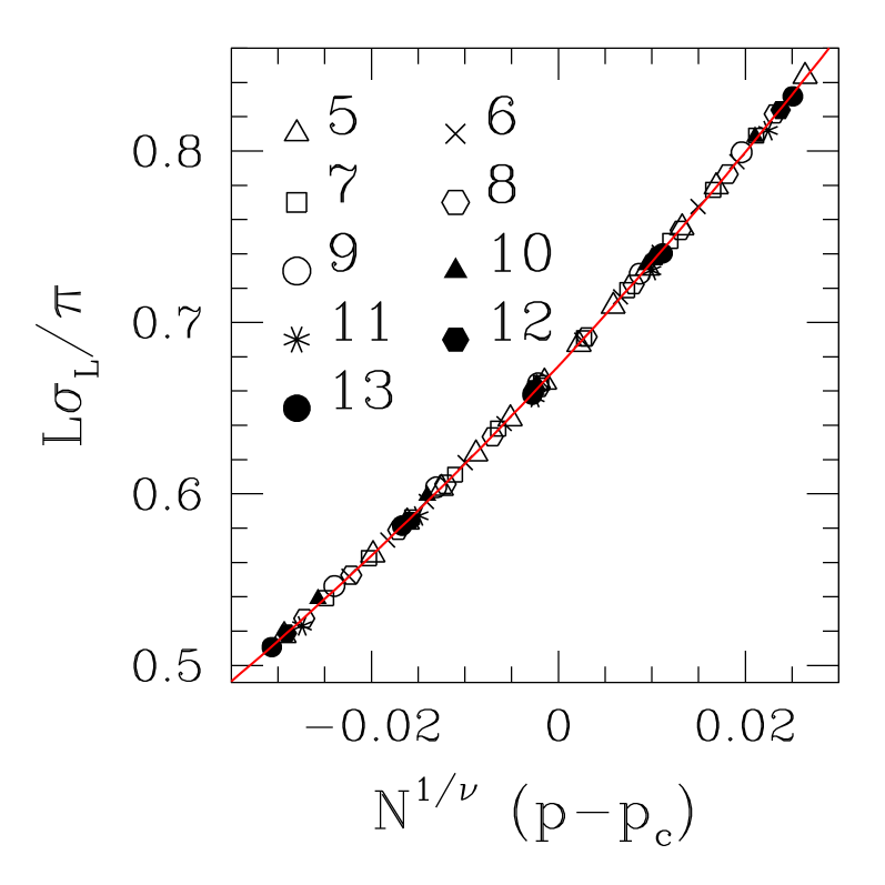
Figure 2: (Color online) Triangular lattice: scaling plot of domain-wall free energies, Eq. (6), against the finite-size scaling variable, $N^{1/\nu}\,(p-p_{c})$. The central estimates $1/\nu=0.67$, $p_{c}=0.8355$, have been used. Full line is quadratic fit to data, from which $\eta=0.674(11)$ (see text).

Standard finite-size scaling Barber (1983) suggests that the curves of Fig. 1 would coincide when plotted against $x\equiv N^{1/\nu}\,(p-p_{c})$.

A quantitative measure of how good the data collapse is can be provided as follows. For trial values of $(\nu,p_{c})$ one calculates the $\chi^{2}$ per degree of freedom ($\chi^{2}_{\rm\ d.o.f.}$) of a fit of the data to a phenomenological baseline curve $f(x)$ (in the present case, since the curvature of data was monotonic, we found a parabolic form to be satisfactory). As the fractional uncertainties of data points were all of the same order, we used unweighted fits, i.e., the $\chi^{2}_{\rm\ d.o.f.}$ was calculated via

$$\chi^{2}_{\rm\ d.o.f.}=(N_{d}-M)^{-1}\sum_{i=1}^{N_{d}}\left(y_{i}-f(x_{i})\right)^{2}\ ,$$ (8)

where $N_{d}$ stands for the number of data, $N_{d}-M$ is the number of degrees of freedom ($M$ is the number of free parameters), $(x_{i},y_{i})$ are the data points, and $f(x_{i})$ are the values of the fitting function at the respective $x_{i}$. The use of uweighted fits is justified because all data used in each fit have similar fractional uncertainties. Therefore, the comparative analysis of different fitting parameters for a specified set of data will not suffer from distortions. This was the procedure used in all data collapse analyses in the present work.

For domain-wall energies on the T lattice, we have found that the best collapse occurs for $1/\nu=0.67(1)$, $p_{c}=0.8355(5)$. For the central estimates the $\chi^{2}_{\rm\ d.o.f.}$ is $3\times 10^{-6}$. Within the intervals of confidence given , the $\chi^{2}_{\rm\ d.o.f.}$ remains below $10^{-5}$. Fig. 2 illustrates the quality of plot obtained, when the central estimates just quoted are used. A parabolic fit to the scaled data gives $\eta=0.674(11)$, where uncertainties in $1/\nu$ and $p_{c}$ have been taken into account, in addition to those intrinsic to the fitting process for fixed values of these parameters.

A similar line of analysis was followed for the HC lattice. Fig. 3 shows the unscaled domain-wall energy data, while Fig. 4 is a scaling plot for the same data. The best collapse occurs for $1/\nu=0.67(1)$, $p_{c}=0.9325(5)$. For the central estimates the $\chi^{2}_{\rm\ d.o.f.}$ is $7\times 10^{-6}$. Within the intervals of confidence given, the $\chi^{2}_{\rm\ d.o.f.}$ remains below $2\times 10^{-5}$. An estimate of $\eta$ from parabolic fits, with the same considerations used for the T lattice, gives $\eta=0.678(15)$.

Figure 3: Honeycomb lattice: domain-wall free energies, Eq. (6), along the NL (parametrized by $p$, see Eq. (2)). Error bars are of order of, or smaller, than symbol sizes.

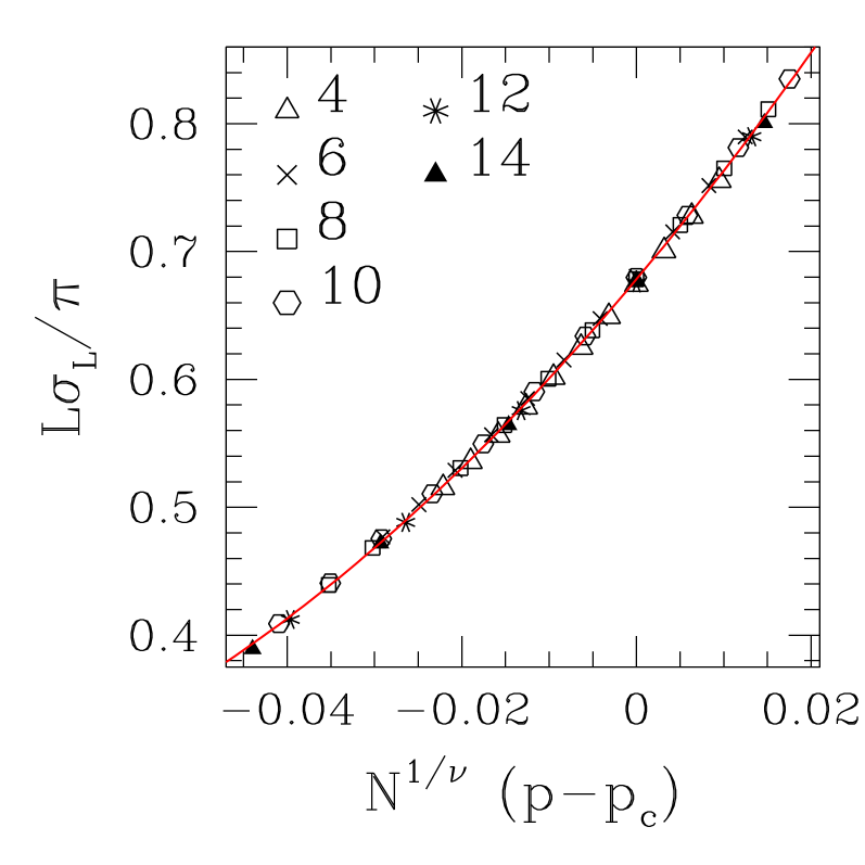
Figure 4: (Color online) Honeycomb lattice: scaling plot of domain-wall free energies, Eq. (6), against the finite-size scaling variable, $N^{1/\nu}\,(p-p_{c})$. The central estimates $1/\nu=0.67$, $p_{c}=0.9325$, have been used. Full line is quadratic fit to data, from which $\eta=0.678(15)$ (see text).

The above estimates of $p_{c}$ for T and HC lattices, when plugged into Eq. (4), result in:

$$H(p_{1c})+H(p_{2c})=1.002(3)\ .$$ (9)

This improves on the accuracy of the estimate given in Ref. Takeda et al., 2005 by one order of magnitude, while still being compatible with the prediction Eq. (5). We view this agreement as a strong indication of plausibility of the conjecture exhibited in Ref. Takeda et al., 2005.

As regards the correlation-length exponent, our estimate $\nu=1.49(2)$ is incompatible with $\nu=1.33(3)$ quoted from the same sort of domain-wall scaling analysis applied to the NP on a square lattice Honecker et al. (2001), but agrees well with $\nu=1.50(3)$, found from mapping into a network model for disordered noninteracting fermions, via TM Merz and Chalker (2002a).

Turning now to the exponent $\eta$ given in Eq. (6), it has been recalled, e.g., in Ref. Merz and Chalker, 2002b, that in the presence of disorder, the scaling indices of the disorder correlator (i.e., the interfacial tension) differ from those of its dual, the order correlator (namely, spin-spin correlations). Nevertheless, the constraints of conformal invariance still hold, with the result that the amplitude of the domain wall energy remains a bona fide universal quantity Merz and Chalker (2002b). For a square lattice, recent estimates give $\eta=0.691(2)$ Honecker et al. (2001); Merz and Chalker (2002a, b). This is slightly outside the error bars quoted here for the T lattice, but within the uncertainty given for HC data.

III Uniform susceptibilities

We calculated uniform zero-field susceptibilities along the NL for both T and HC lattices, similarly to previous investigations on the square lattice Aarão Reis et al. (1999). For the finite differences used in numerical differentiation, we used a field step $\delta h=10^{-4}$ in units of $J_{0}$. As in Sec. II, we took the respective intervals quoted in Ref. Takeda et al., 2005 as a starting guess for the location of the NP.

Finite-size scaling arguments Barber (1983) suggest a form

$$\chi_{N}=N^{\gamma/\nu}\,f\left(N^{1/\nu}(p-p_{c})\right)\ ,$$ (10)

where $\chi_{N}$ is the finite-size susceptibility, and $\gamma$ is the susceptibility exponent. In order to reduce the number of fitting parameters, we kept $1/\nu$ and $p_{c}$ fixed at their central estimates obtained in Sec. II, and allowed $\gamma/\nu$ to vary.

Within this framework, our best fit for the T lattice was for $\gamma/\nu=1.795(20)$, as shown in Fig. 5. For the central estimate the $\chi^{2}_{\rm\ d.o.f.}$ is $1\times 10^{-4}$. Within the intervals of confidence given, the $\chi^{2}_{\rm\ d.o.f.}$ remains below $3\times 10^{-4}$. These deviations are one and a half orders of magnitude larger than the corresponding ones for domain-wall scaling (see Sec. II).

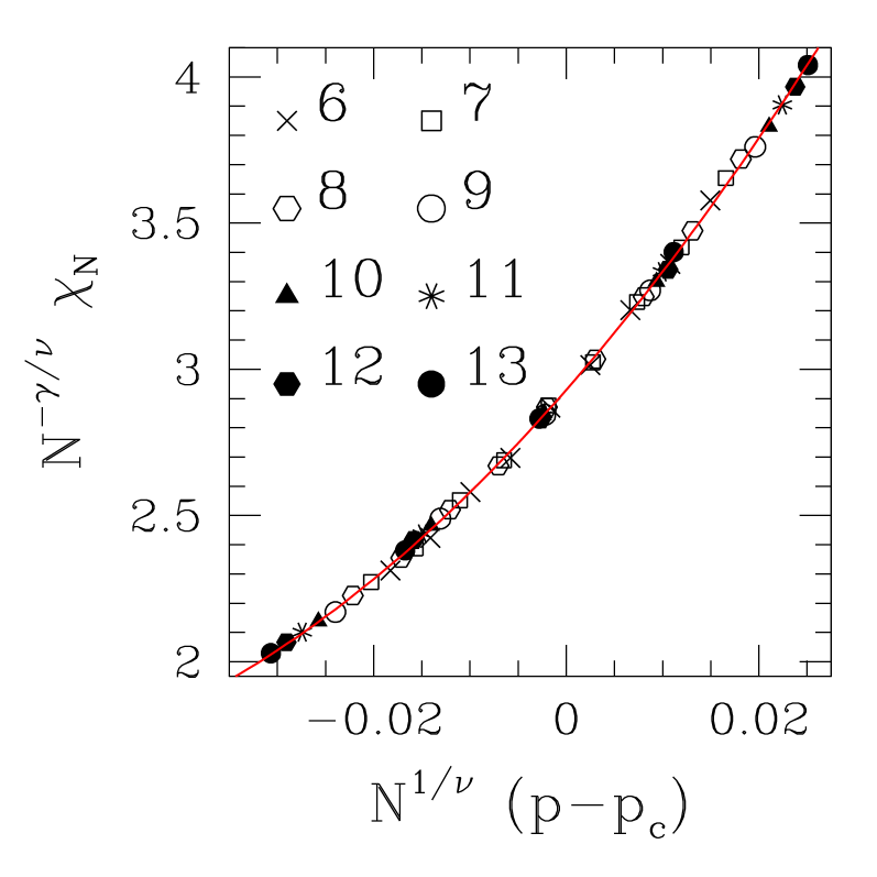
Figure 5: (Color online) Triangular lattice: scaling plot of uniform zero-field susceptibilities, Eq. (10). The central estimates $1/\nu=0.67$, $p_{c}=0.8355$, $\gamma/\nu=1.795$, have been used. Full line is quadratic fit to data.

We repeated the same steps for the HC lattice, with the results displayed in Fig. 6. The best fit now was for $\gamma/\nu=1.80(4)$. For the central estimate the $\chi^{2}_{\rm\ d.o.f.}$ is $1\times 10^{-2}$, two orders of magnitude larger than for the T lattice. The lower quality of adjustment can be witnessed visually. Within the intervals of confidence given, the $\chi^{2}_{\rm\ d.o.f.}$ remains below $3\times 10^{-2}$.

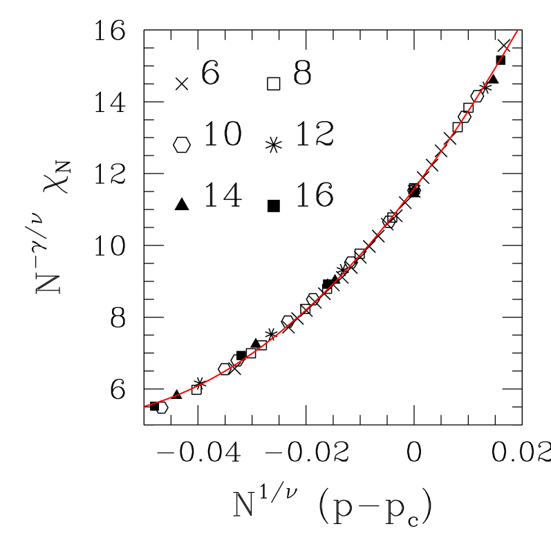
Figure 6: (Color online) Honeycomb lattice: scaling plot of uniform zero-field susceptibilities, Eq. (10). The central estimates $1/\nu=0.67$, $p_{c}=0.9325$, $\gamma/\nu=1.80$, have been used. Full line is quadratic fit to data.

Though the central estimates for the T and HC lattices are very close, the corresponding error bars differ by a factor of two. For the square lattice, we quote $\gamma/\nu=1.80(2)$ Aarão Reis et al. (1999), compatible with both values found here.

IV Correlation functions

Our study of correlation functions is based on previous work for the square lattice de Queiroz and Stinchcombe (2003). We recall the following property, which has been shown to hold on the NL, for correlation functions $C_{ij}$ between Ising spins $\sigma_{i}$, $\sigma_{j}$ Nishimori (1981, 2001, 1986, 2002):

$$[\,C_{ij}^{\,(2\ell+1)}]\equiv[\,\langle\sigma_{i}\sigma_{j}\rangle^{2\ell+1}]=[\,C_{ij}^{\,(2\ell+2)}]\equiv[\,\langle\sigma_{i}\sigma_{j}\rangle^{2\ell+2}]\ ,$$ (11)

where angled brackets indicate the usual thermal average, square brackets stand for configurational averages over disorder, and $\ell=0,1,2,\dots$. Denoting by $P(C_{ij})$ the probability distribution function for the $C_{ij}$, the pairing of successive odd and even moments predicted in Eq. (11) implies that $P^{\prime}(C_{ij})\equiv(1-C_{ij})\,P(C_{ij})$ must be an even function of $C_{ij}$, everywhere on the NL de Queiroz and Stinchcombe (2003). We have explicitly checked that this constraint is obeyed by the distributions generated for the T and HC lattices, within the same degree of accuracy as reported in Ref. de Queiroz and Stinchcombe, 2003 for the square lattice. We shall not deal directly with the $P(C_{ij})$ in what follows; instead, we concentrate on the scaling of their assorted moments $m_{\,k}\equiv[\,C_{ij}^{\,k}]$ , especially in connection with their conformal-invariance properties.

In contrast to the symmetry exhibited in Eq. (11) which holds everywhere on the NL, conformal invariance is expected only where the NL crosses the phase boundary, i.e., at the NP.

For pure Ising systems on a strip of width $L$ of a square lattice, with periodic boundary conditions across, conformal invariance implies that at criticality, the correlation function between spins located respectively at the origin and at $(x,y)$ behaves as Cardy (1987):

$$C_{xy}^{\rm pure}\sim\left[\frac{\pi/L}{\left[\sinh^{2}(\pi x/L)+\sin^{2}(\pi y/L)\right]^{1/2}}\right]^{\eta}\ ,\ \eta=1/4\ .$$ (12)

For the T and HC lattices, the same is true, provided that the actual, i.e., geometric site coordinates along the strip are used in Eq. (12). Thus, from the representation of the T lattice as a square (SQ) lattice with a single diagonal bond, and of the HC as a “brick" lattice, the respective SQ-like integer coordinates $(i,j)$ transform respectively into

$$x=\frac{\sqrt{3}}{2}\,i\ ;\ y=j-\frac{1}{2}\,i\qquad{\rm(T)}\ ;$$

$$x=\sqrt{3}\,i\ ;\ y=j+\bigl{[}\,\frac{j+1}{2}\,\bigr{]}\qquad{\rm(HC)}\ ,$$ (13)

where $[X]$ denotes the largest integer contained in $X$. Recall that $L=N$ (T); $L=3N/2$ (HC), as explained above. With $R\equiv(x^{2}+y^{2})^{1/2}$, the proportionality factor in Eq. (12) can be obtained from exact results ($L,R\to\infty,\ R\ll L$), $C_{R}=A_{\rm X}/R^{1/4}$, where $A_{\rm X}=0.703\,38\dots$, $0.668\,65\dots$, $0.767\,04\dots$ respectively for X = SQ, T, HC Hartwig and Stephenson (1968).

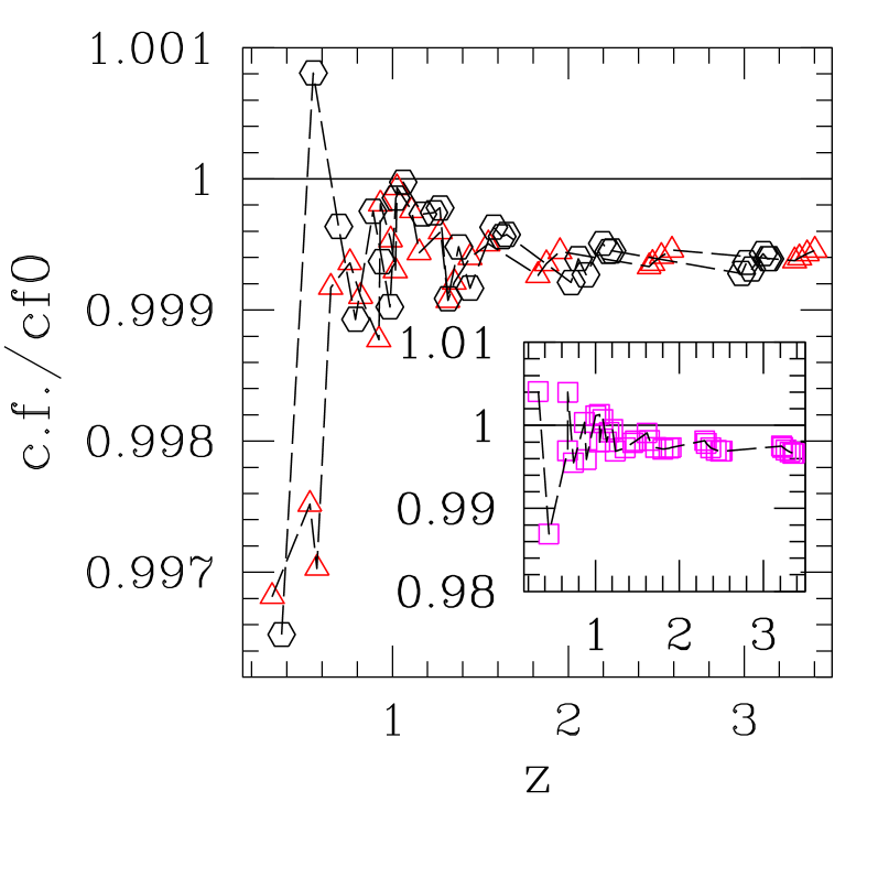
Figure 7: (Color online) Pure systems: ratio of calculated correlation functions at the critical point (c.f.) to asymptotic form given in Eq. (12) (cf0), against $z\equiv(\sinh^{2}(\pi x/L)+\sin^{2}(\pi y/L))^{1/2}$. Main diagram: T lattice (triangles), HC lattice (hexagons). Insert: SQ lattice. Strip width $N=10$ sites, for all cases.

Though strictly speaking Eq. (12) is an asymptotic form, for the SQ lattice discrepancies are already very small at short distances de Queiroz and Stinchcombe (2003), and are even smaller for T and HC, as illustrated in Fig. 7. The horizontal axis in the Figure is the argument $z\equiv(\sinh^{2}(\pi x/L)+\sin^{2}(\pi y/L))^{1/2}$ of Eq. (12). The range of $z$ depicted corresponds to $x/L\lesssim 0.6$, i.e. (for strip width $N=10$ sites) up to, respectively, 5(HC), 6(SQ), or 7 (T) full iterations of the TM. For larger $x/L$ the angular dependence of $z$ (through $y$) becomes less than one part in $10^{2}$. For $z\lesssim 1$ the discrepancy from Eq. (12) is at most $0.4\%$ for both T and HC, while in the worst case for SQ, namely $(x,y)$=(1,1), it reaches $1.3\%$. For $1<z<3$, the difference is $<0.1\%$ for T and HC, and $<0.3\%$ for SQ.

The above analysis of conformal invariance of pure-system correlation functions indicates that, should similar trends hold at the NP of spin glasses, estimates of associated critical indices for T and HC lattices would behave more smoothly than for SQ (since they rely on fits of numerically-calculated correlations to Eq. (12), with $\eta$ as an adjustable parameter). As in earlier work de Queiroz and Stinchcombe (2003), we concentrate on short-distance correlations, i.e., where the argument $z$ is strongly influenced by $y$. Such a setup is especially convenient in order to probe the angular dependence predicted in Eq. (12), which constitutes a rather stringent test of conformal invariance properties.

We now turn to the quantitative analysis of the behavior of assorted moments $m_{i}$ of the correlation-function distribution, against $z$. Bearing in mind Eq. (11), and following Ref. de Queiroz and Stinchcombe, 2003, our goal is to extract the decay-of-correlations exponents $\eta_{\,2j+1}$, via fits of our data to the form $m_{\,2j+1}\sim z^{-\eta_{\,2j+1}}$.

When one attempts such fits, several likely sources of uncertainty are present, on which we now comment. First, one has the finite width $N$ of the strips used. In Ref. de Queiroz and Stinchcombe, 2003, an extensive analysis of this point was undertaken, with the conclusion that, e.g. for $N=10$, finite-width effects are already essentially subsumed in the explicit $L$ (i.e., $N$) dependence of Eq. (12), thus higher-order finite-size corrections most likely do not play a significant role. We shall assume that this is the case here as well, and restrict ourselves to $N=10$ for both T and HC lattices. Second, the finite length $M$ of strips implies that averaged values will fluctuate from sample to sample. Though the distribution itself (of, e.g., correlation functions) displays an intrinsic width which is a non-vanishing feature connected to the lack of self-averaging present at criticality, the average moments of the distribution behave in the expected manner, namely, their sample-to-sample fluctuations approach zero roughly as $\sqrt{M}$ with increasing sample length $M$ de Queiroz and Stinchcombe (1996); Talapov and Shchur (1994). Therefore, from a set of runs at assorted small values of $M$, one can infer what effect sample-to-sample fluctuations will have on results for larger $M$. In the calculation of results shown below, we have used $M=10^{7}$, which implies a total of $M^{\prime}=3.3\times 10^{6}$ non-overlapping samples for our correlation-function statistics (because each sample needs three full iterations of the TM, in order to scan the set of lattice points of interest). For such value of $M$, the estimation procedure just outlined predicts fluctuations of order $0.1\%$, at most.

Finally, one has the uncertainty in the location of the critical point. We have found that, in the present case, this is the main source of uncertainties for our data. Thus, e.g., with $p_{c}=0.8355(5)$ for the T lattice, averaged moments $m_{\,2j+1}$ taken at at the central estimate differ from those calculated at the edge of the error bar, by an amount increasing systematically with $j$, from $\sim 0.7\%$ for $j=0$, to $\sim 1.5\%$ for $j=3$. For HC, deviations follow the same trend against $j$ but are slightly larger, ranging from $\lesssim 1\%$ for $j=0$, to $\lesssim 2\%$ for $j=3$.

In Fig. 8 we show data for the T lattice, taken at our central estimate for the location of the NP, $p=0.8355$. The error bars, associated mainly to the uncertainty in $p_{c}$, as just discussed, are at most of order of the symbol sizes.

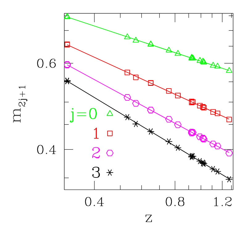
Figure 8: (Color online) Triangular lattice: double-logarithmic plot of odd moments of the correlation-function distribution $P(C_{xy})$ against $z\equiv(\sinh^{2}(\pi x/L)+\sin^{2}(\pi y/L))^{1/2}$ (see Eqs. (12) and  (13)). Straight lines are unweighted least-squares fits to data. Data taken at $p=0.8355$ for strip width $N=10$, $M^{\prime}=3.3\times 10^{6}$ non-overlapping samples in all cases.

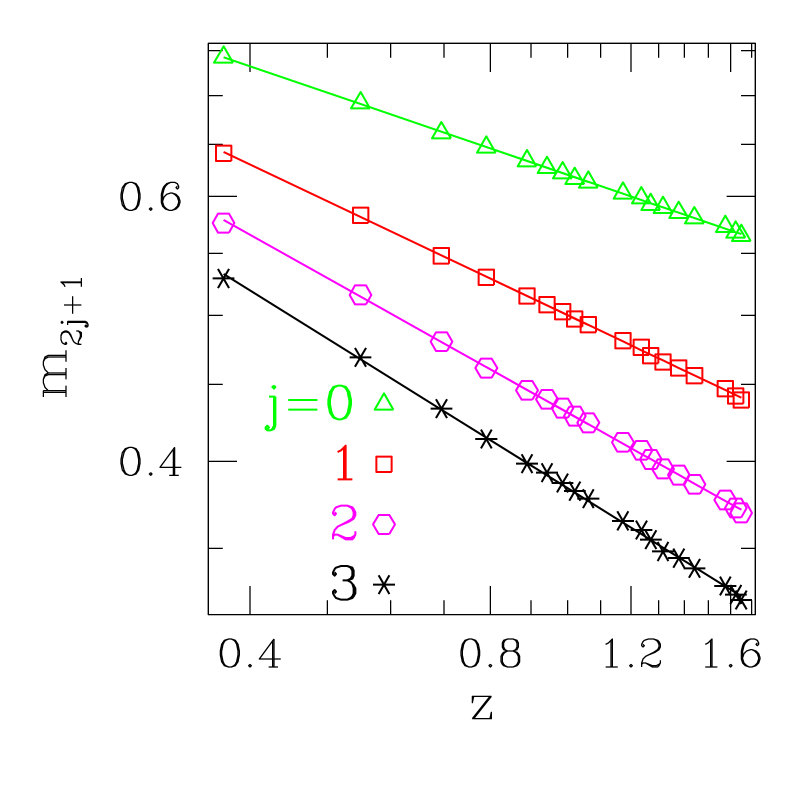
Figure 9: (Color online) Honeycomb lattice: double-logarithmic plot of odd moments of the correlation-function distribution $P(C_{xy})$ against $z\equiv(\sinh^{2}(\pi x/L)+\sin^{2}(\pi y/L))^{1/2}$ (see Eqs. (12) and  (13)). Straight lines are unweighted least-squares fits to data. Data taken at $p=0.9325$ for strip width $N=10$, $M^{\prime}=3.3\times 10^{6}$ non-overlapping samples in all cases.

Fig. 9 exhibits data for the HC lattice. Pertinent comments are similar to those made above for the T lattice.

Table 1: Estimates of exponents $\eta_{\,2j+1}$, from least-squares fits of averaged odd moments of correlation-function distributions. Data for $N=10$ and $z\lesssim 1.6$, assuming $m_{2j+1}\sim z^{-\eta_{\,2j+1}}$. T: triangular lattice (this work); HC: Honeycomb lattice (this work); SQ: square lattice, calculated at the conjectured exact location of the NP, see Eq. (3) (Ref. de Queiroz and Stinchcombe, 2003). Last two columns: square lattice, authors as quoted.

$j$	T	HC	SQ	Ref. Honecker et al.,2001	Ref. Merz and Chalker,2002a
0	0.181(1)	0.181(1)	0.1854(17)	0.1854(19)	0.183(3)
1	0.251(1)	0.252(1)	0.2556(20)	0.2561(26)	0.253(3)
2	0.297(2)	0.296(2)	0.300(2)	0.3015(30)	–
3	0.330(2)	0.329(3)	0.334(3)	0.3354(34)	–

In Table 1 we give numerical results of the fits illustrated in Figs. 8 and 9. Though T and HC estimates are quite consistent with each other, and with the results of Ref. Merz and Chalker, 2002a, for $j=0$ and $1$ both fall slightly below their SQ counterparts given in Refs. de Queiroz and Stinchcombe, 2003; Honecker et al., 2001. For $j=2$ and $3$, as a consequence of generally wider error bars, all estimates are broadly compatible with one another.

V Discussion and Conclusions

We have used domain-wall scaling techniques in Sec. II to determine the location of the Nishimori point of Ising spin glasses on both the T and HC lattices. Probing the temperature–concentration plane along the Nishimori line, we have obtained well-behaved curves of interfacial free energy; with the help of standard finite-size scaling techniques, we have extracted the estimates $p_{c}=0.8355(5)$ and $p_{c}=0.9325(5)$ respectively for the location of the Nishimori point on T and HC lattices. As a consequence of this, we have been able to refine the estimate of the quantity $H(p_{1c})+H(p_{2c})$ (see Eqs. (4) and (5)), which has been conjectured in Ref. Takeda et al., 2005 to be exactly unity. Indeed, our result given in Eq. (9) is $1.002(3)$, which gives strong support to the conjecture cited.

Furthermore, interfacial free energy data have allowed us to estimate the correlation-length exponent to be $\nu=1.49(2)$, in very good agreement with $\nu=1.50(3)$ from a mapping of the problem into a network model for disordered noninteracting fermions Merz and Chalker (2002a), but incompatible with $\nu=1.33(3)$ from a TM treatment, presumably very similar to the present one, for the SQ lattice Honecker et al. (2001).

In order to investigate whether this latter disagreement might indicate a lattice-dependent breakdown of universality, we calculated domain-wall free energies on the SQ lattice as well. Strip widths $N=4-12$ (both even and odd) were used, again with $M=2\times 10^{6}$ columns (except for $N=12$ where $M=1\times 10^{6}$). We scanned the region of the NL comprising $0.88\lesssim p\lesssim 0.90$, which includes both the conjectured exact location of the NP Nishimori and Nemoto (2002); Maillard et al. (2003), namely $p_{c}=0.889972\cdots$, and the estimate given in Ref. Honecker et al., 2001, $p_{c}=0.8906(2)$. We found that scaled data collapse more smoothly for $p_{c}$ and $\nu$ respectively close to $0.889972\cdots$ and $1.5$, rather than the values quoted in Ref. Honecker et al., 2001. This is illustrated in Fig. 10, which exhibits the $\chi^{2}_{\rm\ d.o.f}$ for unweighted quadratic fits of scaled domain-wall energies to a dependence on the finite-size scaling variable $N^{1/\nu}\,(p-p_{c})$, plotted against $1/\nu$. Each set of data corresponds to fixed $p_{c}$, see caption to the Figure. We obtain $\nu=1.45(8)$, $p_{c}=0.8900(5)$, where the intervals of confidence given reflect the region in $(\nu,p_{c})$ parameter space in which the $\chi^{2}_{\rm\ d.o.f}$ remains below $\sim 1.5$ times its overall minimum. Though the error bar for $\nu$ is double that for T and HC lattices, the present estimate still encompasses the respective results for both, while excluding $\nu=1.33$. For the domain-wall energy amplitude, we quote $\eta=0.665(10)$, slightly lower than, but still compatible with, the values found in Sec. II. We conclude that our domain-wall energy data fully support a picture of universal (i.e., lattice-independent) behavior at the NP of T, HC, and SQ lattices. For all three lattices the correlation-length exponent is consistent with $\nu=1.50(3)$ of Ref. Merz and Chalker, 2002a, but most likely excludes $\nu=1.33(3)$ of Ref. Honecker et al., 2001.

Figure 10: Square lattice: semi-logarithmic plots of $\chi^{2}_{\rm\ d.o.f}$ for (unweighted) quadratic fits of domain-wall energies on SQ lattice to a dependence on the finite-size scaling variable $N^{1/\nu}\,(p-p_{c})$, against $1/\nu$. Each set of data corresponds to fixed $p_{c}$, as follows: triangles, $p_{c}=0.889972$ (conjectured exact, Refs. Nishimori and Nemoto, 2002; Maillard et al., 2003); squares, $p_{c}=0.8894$; hexagons, $p_{c}=0.8897$; stars, $p_{c}=0.8903$; crosses, $p_{c}=0.8906$ (central estimate of Ref. Honecker et al., 2001). Strip widths $4\leq N\leq 12$.

Our data for the uniform susceptibility, exhibited in Sec. III, do not scale as smoothly as the domain-wall energies. Nevertheless, the application of finite-size scaling ideas yields estimates for the exponent ratio $\gamma/\nu$ which strongly support universal behavior at the NP, for T, HC, and SQ lattices. We recall that early work characterized the transition at the NP as compatible with the universality class of random percolation (see, e.g., Refs. Aarão Reis et al., 1999; Honecker et al., 2001; de Queiroz and Stinchcombe, 2003 for discussions of this point). In this context, we note that even our most accurate single result, namely $\gamma/\nu=1.795(20)$ for the T lattice, does not rule out the percolation value Stauffer and Aharony (1994) $(\gamma/\nu)_{p}=43/24=1.7917\dots$. However, as explained below, consideration of the full set of results obtained here does support a scenario which rules out percolation-like behavior.

Next, we turn to the investigation of correlation functions in Sec. IV. The rapid convergence of T and HC results towards the asymptotic form, illustrated in Fig. 7 for pure systems, has translated to some extent into a discernible improvement on the accuracy of estimates for the disordered case. As explained above, for spin glasses on T and HC lattices the uncertainty in the location of the NP is the main source of fluctuations in numerically-calculated quantities. Thus, the relatively small uncertainties shown in Table 1 show that the former effect compensates for the noise associated to the latter, at least partially. Compare, e.g., the T and HC columns with that for data taken at the conjectured exact location of the NP on SQ de Queiroz and Stinchcombe (2003).

The overall picture summarized in Table 1 clearly points towards universality of the several (multifractal) Merz and Chalker (2002a, b) decay-of-correlation exponents. The small discrepancies observed, for $j=0$ and $1$, between the T and HC estimates, and a subset of those obtained earlier for SQ, are likely to depend on details of the respective fitting procedures. One must note, however, that the $j=0$ and $1$ T and HC estimates are consistent with those derived in Ref. Merz and Chalker, 2002a. This is similar to the case for the exponent $\nu$, in which our own result is compatible with the value found in Ref. Merz and Chalker, 2002a, and not with that given in Ref. Honecker et al., 2001.

Focusing now on $j=0$, an unweighted average of all results of the corresponding line in Table 1 gives $\eta_{1}=0.183(3)$. Considering the scaling relation $\gamma/\nu=2-\eta_{1}$, one gets $\gamma/\nu=1.817(3)$, which excludes $(\gamma/\nu)_{p}$ by a broad margin. Therefore, we quote the set of exponents $\nu=1.49(2)$, $\gamma=2.71(4)$ $\eta_{1}=0.183(3)$, distinctly different from the percolation values Stauffer and Aharony (1994) $\nu_{p}=4/3$, $\gamma_{p}=43/18$, $\eta_{p}=5/24$.

In summary, we have (i) produced accurate estimates of the location of the NP on T and HC lattices, which provide strong evidence in support of the conjecture expressed in Eq. (5); (ii) confirmed that the critical properties of the NP in two-dimensional systems are universal in the expected sense; and (iii) provided further evidence that such properties belong to a distinct universality class from that of percolation.

As a final remark, we note that our discussion has been restricted to critical behavior upon crossing the ferro-paramagnetic phase boundary. The critical properties along the boundary line are of interest as well Aarão Reis et al. (1999); Merz and Chalker (2002a), and their investigation on the T and HC lattices would be a natural continuation of the present work.