Static and dynamic properties of crystalline phases of two-dimensional electrons
in a strong magnetic field

Abstract

We study the cohesive energy and elastic properties as well as normal modes of the Wigner and bubble crystals of the two-dimensional electron system (2DES) in higher Landau levels. Using a simple Hartree-Fock approach, we show that the shear moduli ($c_{66}$’s) of these electronic crystals show a non-monotonic behavior as a function of the partial filling factor $\nu^{*}$ at any given Landau level, with $c_{66}$ increasing for small values of $\nu^{*}$, before reaching a maximum at some intermediate filling factor $\nu^{*}_{m}$, and monotonically decreasing for $\nu^{*}>\nu^{*}_{m}$. We also go beyond previous treatments, and study how the phase diagram and elastic properties of electron solids are changed by the effects of screening by electrons in lower Landau levels, and by a finite thickness of the experimental sample. The implications of these results on microwave resonance experiments are briefly discussed.

I Introduction

There has been much interest recently, both theoretically and experimentally, in the quantum phases of the two-dimensional electron system in higher Landau levels (LLs). Hartree-Fock (HF) studiesFogler1996 ; Moessner1996 have shown that, for small partial filling factors $\nu^{*}=\nu-2n\approx 0.1-0.2$ (with $\nu$ the total filling factor and $n$ the Landau level index), the electrons form a triangular Wigner crystal (WC), while for $\nu^{*}$ close to $1/2$ the ground state of the system is a unidirectional charge density wave or “stripe” state.Fogler1996 Between these two regions, HFFogler1996 ; Cote2003 ; Goerbig2004 and density matrix renormalization group (DMRG) methods,Shibata2001 as well as exact diagonalization on small systems,Haldane2000 have suggested the existence of a new kind of crystal structure, the “bubble crystal” (BC), with more than one electron per lattice cell. While HF predicts transitions between bubble phases with increasing number $M$ of electrons per bubble, with $M$ going up to $M=n+1$ electrons in LL $n$, in DMRG the last bubble phase is absent, and a transition takes place directly from the BC with $M=n$ electrons per bubble to the stripe state. It is noteworthy that the difference in cohesive energy between all these different phases remains very small, of order $0.01-0.03e^{2}/\epsilon\ell$ (with $e$ the electronic charge, $\epsilon$ the dielectric constant of the host semiconductor and $\ell$ the magnetic length).

On the experimental side, evidence for the existence of these different phases is found mainly through transport experiments. Early DC measurementsLilly1999 ; Du1999 have shown strongly anisotropic transport around half-filling, which was interpreted as evidence for a stripe state. Crystal phases of electrons, which are pinned by quenched disorder, should all be insulating in the DC regime. One has therefore to resort to other experimental techniques to resolve the transitions between these different crystal phases (e.g. WC to BC). One particular such technique consists in measuring the microwave response of the 2DES, which would give different resonant behavior for different electronic crystalline phases. While early microwave conductivity experimentsChen2003 ; Lewis2003 gave considerable support to the existence of a WC around integer filling $\nu=1,2,3$ and $4$ for $\nu^{*}<1/2$, it was not until recently that coexistence between two phases with two distinct resonant peaks was observed by Lewis et al.Lewis2004 . It is our aim in this paper to discuss in some detail the experimental results of this last reference, in light of recent advances in resonance pinning theories of two-dimensional electronic solids.Chitra2001 ; Fogler2000 In order to do so, we will need to develop a microscopic picture of the 2DES as a system of interacting guiding centers. Indeed, after projection of the electronic density on the uppermost Landau level the problem at hand reduces to one of interacting guiding centers (of quenched kinetic energy) with an appropriately defined effective interaction potential that includes quantum effects at the Hartree-Fock level. The knowledge of the effective interaction potential between guiding centers will allow us to find the elastic moduli and the normal eigenmodes of the Wigner and bubble crystals. In agreement with the results of Maki and ZotosMaki1983 for the WC in the lowest LL, we find that the shear moduli ($c_{66}$’s) of the Wigner and bubble crystals show a non-monotonic behavior as a function of the partial filling factor $\nu^{*}$ at any given Landau level, with $c_{66}$ increasing for small values of $\nu^{*}$, before reaching a maximum at some intermediate filling factor $\nu^{*}_{m}$, and then monotonically decreasing for $\nu^{*}>\nu^{*}_{m}$. These results will allow us to attempt a qualitative analysis of recent microwave experiments by Lewis et al.Lewis2004 . We find that, while the $\nu^{*}$ behavior of the first resonance peak observed in this last reference is in good qualitative agreement with existing theoretical predictions for the pinned Wigner crystal,Chitra2001 the second resonance peak has a behavior as a function of $\nu^{*}$ which is quite different from what a linearized solution of self-consistent equations for the microwave response theories predict for the two-electron bubble state. Below, we shall argue that an adequate description of the resonance peak of bubble crystals may require the full numerical solution of the self-consistent response equations, as done in Ref. Cote2005, .

This paper is organized as follows. In Sec. II we review the physics of the Wigner crystal and bubble states, and introduce some notation. In Sec. III we find the shear moduli of the Wigner and bubble crystals in LLs $n=2$ and $n=3$. In Sec. IV we calculate the normal modes of the Wigner crystal and of the two-electron bubble solid in the Landau level $n=2$. Then, in Sec. V we investigate the effect of screening by lower LLs and of finite sample thicknesses on the cohesive energies and shear moduli of the Wigner and bubble crystals in LLs $n=2$ and $n=3$. In Sec.VI we discuss the implications of our results for the shear moduli on the microwave response of electronic crystals in light of the recent microwave conductivity experiments of Lewis et al.Lewis2004 Finally, Sec. VII contains a summary of our results along with our conclusions.

II Wigner crystal and bubble phases in higher Landau levels: Hartree-Fock approach

We shall start from the expression of the Hartree-Fock Hamiltonian of the $n$-th partially filled Landau level, which is given by (throughout this paper, we use $\int_{\bf q}$ as a shorthand for $\int\frac{d^{2}\bf q}{(2\pi)^{2}}$)

$$H_{HF}=\frac{1}{2}\int_{\bf q}V_{HF}({\bf q})|\rho({\bf q})|^{2},$$ (1)

where $V_{HF}$ is the Hartree-Fock interaction, and $\rho({\bf q})$ is the projection of the electronic density $n({\bf q})$ onto the uppermost LL, and is given by

$$\rho({\bf q})=\frac{n({\bf q})}{e^{-q^{2}\ell^{2}/4}L_{n}(q^{2}\ell^{2}/2)}.$$ (2)

For a bubble crystal with $M$ electrons per bubble, we shall approximate the electronic density by

$$n({\bf r})=\sum_{i}\sum_{m=0}^{M-1}|\varphi_{n,m}({\bf r}-{\bf R}_{i})|^{2},$$ (3)

where $\varphi_{n,m}({\bf r})$ is the noninteracting wavefunction of angular momentum $m$ and Landau level index $n$, and where the summation extends over all the bubbles located at the lattice sites ${\bf R}_{i}$ of a triangular Bravais lattice and over all the electrons within each bubble. The Hartree-Fock interaction potential in Eq. (1) consists of the sum of a Hartree and Fock parts, which are given, in the Landau gauge ${\bf A}=Bx\hat{\bf y}$ (${\bf A}$ being the vector potential), by Cote2003 ; Goerbig2004

$$V_{H}({\bf q})=\frac{2\pi e^{2}}{\epsilon q}\mbox{e}^{-q^{2}\ell^{2}/2}\big{[}L_{n}(q^{2}\ell^{2}/2)\big{]}^{2},$$ (4a)

$$V_{F}({\bf q})=-(2\pi\ell^{2})\;\int_{{\bf q}^{\prime}}V_{H}({\bf q}^{\prime})e^{-i{\bf q}\times{\bf q}^{\prime}\ell^{2}},$$ (4b)

where $L_{n}(x)$ is the $n$-th Laguerre polynomial.

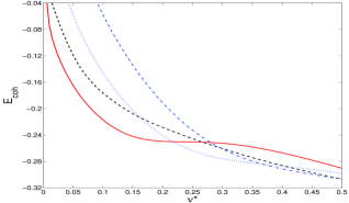
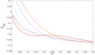
Figure 1: (Color online) Cohesive energy of the Wigner crystal (solid line), $M=2$ (dotted line), $M=3$ (thin dash-dotted line) and $M=4$ bubble solids (thick dash-dotted line in the lower panel). The cohesive energy of the stripe state is indicated by a dashed line, and all cohesive energies are in units of $e^{2}/\epsilon\ell$. The upper panel is for $n=2$, and the lower panel is for $n=3$.

The calculation of the cohesive energy of the Wigner crystal and bubble phases proceeds in a standard way as follows. From Eqs. (2) and (3), it is easy to see that we can write the projected density $\rho({\bf q})$ in the form

$$\rho({\bf q})=\tilde{\rho}({\bf q})\sum_{i}e^{-i{\bf q}\cdot{\bf R}_{i}},$$ (5)

where the sum runs through all vectors ${\bf R}_{i}$ of the triangular Bravais lattice, and where $\tilde{\rho}({\bf q})$ is given by

$$\tilde{\rho}({\bf q})=\frac{\tilde{n}({\bf q})}{e^{-q^{2}\ell^{2}/4}L_{n}(q^{2}\ell^{2}/2)},$$ (6)

with $\tilde{n}({\bf q})$ the Fourier transform of the density at a given bubble,

$$\tilde{n}({\bf q})=\sum_{m=0}^{M-1}\int d{\bf r}|\varphi_{nm}({\bf r})|^{2}e^{-i{\bf q}\cdot{\bf r}}.$$ (7)

Inserting the decomposition (5) into the expression of the cohesive energy, Eq. (1), and making use of Poisson’s summation formula (here $A_{c}=2\pi\ell^{2}M/\nu^{*}$ is the area of the unit lattice cell and the ${\bf Q}$’s are reciprocal lattice vectors)

$$\sum_{i}e^{-i{\bf q}\cdot{\bf R}_{i}}=\frac{(2\pi)^{2}}{A_{c}}\sum_{\bf Q}\delta({\bf q}-{\bf Q}),$$ (8)

we finally obtain the following expression for the cohesive energy per particle $E_{coh}=\langle H_{HF}\rangle/N$ :

$$E_{coh}=\frac{1}{2A_{c}}\sum_{\bf Q}\big{[}V_{H}({\bf Q})(1-\delta_{{\bf Q},{\bf 0}})+V_{F}({\bf Q})\big{]}|\tilde{\rho}({\bf Q})|^{2},$$ (9)

where charge neutrality requires that we exclude the diverging ${\bf Q}=0$ Hartree term from the summation. In Fig. 1, we show the cohesive energies of the different phases (Wigner crystal, bubble solids and stripes) in the Landau levels $n=2$ and $n=3$. The values of the cohesive energies shown, and of the partial filling factor $\nu^{*}$, at which transitions between the different phases occur in both Landau levels, are in excellent agreement with recent Hartree-Fock calculations by Côté et al.Cote2003 and by Goerbig et al.Goerbig2004 As it can be seen, the energy difference between the WC, BC and stripe states is extremely small, of order $0.02e^{2}/\epsilon\ell$, which is within the range of the magnetophonon and magnetoplasmon excitation spectrum of these phases. It is therefore conceivable that quantum fluctuations, in the form of zero-point energy, may alter the cohesive energies and therefore change the structure of the phase diagram of the 2DES in higher LLs. This point will be investigated in Sec. IV, where we shall write an equation of motion for the electron guiding centers in the Wigner and bubble crystals, with the goal of finding the normal eigenmodes (and hence the zero-point energy) of these structures. An essential ingredient in such a calculation is the elastic matrix of the Wigner and bubble crystals, that we shall determine in Sec. III below.

III Elastic matrix and elastic moduli of the Wigner and bubble crystals in higher Landau levels

Having reviewed the basic phase diagram of the 2D electron gas in partially filled LLs, we now would like to study the elastic properties of the Wigner and bubble crystals. But, in order to be able to do so, we still need to derive an effective interaction between the guiding centers of the electrons, which in turn will allow us to derive the elastic matrix of the WC and BC, and hence find the compression and shear moduli of these crystalline structures. This will be the object of the following Subsection.

III.1 Effective interaction potential between guiding centers

Going back to Eqs. (5)-(7), if we furthermore write for the projected density $\tilde{\rho}({\bf q})$ the decomposition $\tilde{\rho}({\bf q})=\sum_{m}\tilde{\rho}_{m}({\bf q})$, with

$$\tilde{\rho}_{m}({\bf q})=\frac{\int d{\bf r}|\varphi_{nm}({\bf r})|^{2}e^{-i{\bf q}\cdot{\bf r}}}{e^{-q^{2}\ell^{2}/4}L_{n}(q^{2}\ell^{2}/2)},$$ (10)

then we can rewrite the cohesive energy $E_{HF}$ in the form

$$E_{HF}=\frac{1}{2}\sum_{\underset{m,m^{\prime}}{i\neq j}}U_{mm^{\prime}}({\bf R}_{i}-{\bf R}_{j})+\!\!\!\sum_{i,m<m^{\prime}}U_{mm^{\prime}}(0),$$ (11)

where we introduced the effective interaction potential $U_{mm^{\prime}}$ between guiding centers of electrons in states $m$ and $m^{\prime}$, which in real space is given by

$$U_{mm^{\prime}}({\bf r})=\int_{\bf q}\tilde{\rho}_{m}({\bf q})V_{HF}({\bf q})\tilde{\rho}_{m^{\prime}}({\bf q})e^{i{\bf q}\cdot{\bf r}}.$$ (12)

In the following Subsection, we shall use the above expression of the interaction potential to study the normal modes of the bubble crystal in higher ($n\geq 2$) LLs.

III.2 Elastic moduli of the electron crystal

The derivation of the elastic moduli associated with the effective interaction potential in Eq. (12) proceeds in a standard way as follows. First, we evaluate the elasticity matrix $\Phi_{\alpha\beta}({\bf R})$, which is given byAshcroft1988

$$\Phi_{\alpha\beta}({\bf R})=\delta_{{\bf R},{\bf 0}}\sum_{k}\partial_{\alpha}\partial_{\beta}U({\bf R}_{k})-\partial_{\alpha}\partial_{\beta}U({\bf R}),$$ (13)

with $U$ the total interaction potential between bubbles:

$$U({\bf r})=\sum_{m,m^{\prime}}U_{mm^{\prime}}({\bf r}).$$ (14)

Using the following definition of the direct and inverse Fourier transformations (here the ${\bf q}$ integration is carried over the first Brillouin zone of the reciprocal lattice, and we remind the reader that $A_{c}$ is the area of the primitive unit cell of the bubble crystal):

$$\Phi_{\alpha\beta}({\bf q}) = \sum_{\bf R}\Phi_{\alpha\beta}({\bf R})e^{-i{\bf q}\cdot{\bf R}},$$ (15a)

$$\Phi_{\alpha\beta}({\bf R}) = \frac{1}{A_{c}}\int_{\bf q}\Phi_{\alpha\beta}({\bf q})e^{i{\bf q}\cdot{\bf R}},$$ (15b)

and the identity (8), one can easily show that $\Phi_{\alpha\beta}({\bf q})$ can be written in the form

$$\Phi_{\alpha\beta}({\bf q}) = \frac{1}{A_{c}}\sum_{\bf Q}\big{[}(q_{\alpha}+Q_{\alpha})(q_{\beta}+Q_{\beta})U({\bf q}+{\bf Q})$$ (16)

$$- Q_{\alpha}Q_{\beta}U({\bf Q})\big{]}.$$

Expanding the second term on the right hand side of the above equation in $q$ around $q=0$ leads to the result

$$\Phi_{\alpha\beta}({\bf q}) = \frac{1}{A_{c}}q_{\alpha}q_{\beta}\Bigg{\{}U(q)+\sum_{{\bf Q}\neq 0}\Bigg{[}U(Q)+(Q_{\alpha}^{2}+Q_{\beta}^{2})\frac{U^{\prime}(Q)}{Q}+Q_{\alpha}^{2}Q_{\beta}^{2}\Big{(}\frac{QU^{\prime\prime}(Q)-U^{\prime}(Q)}{Q^{3}}\Big{)}\Bigg{]}\Bigg{\}}$$ (17)

$$+ \frac{1}{2A_{c}}\delta_{\alpha\beta}\sum_{{\bf Q}\neq 0}\Big{[}q^{2}Q_{\alpha}^{2}\frac{U^{\prime}(Q)}{Q}+Q_{\alpha}^{2}(q_{x}^{2}Q_{x}^{2}+q_{y}^{2}Q_{y}^{2})\Big{(}\frac{QU^{\prime\prime}(Q)-U^{\prime}(Q)}{Q^{3}}\Big{)}\Big{]}$$

Given that the elastic matrix of a two-dimensional triangular lattice is of the general form

$$\Phi_{\alpha\beta}({\bf q})=(c_{11}-c_{66})q_{\alpha}q_{\beta}+c_{66}q^{2}\delta_{\alpha\beta},$$ (18)

we see that the compression and shear moduli can be extracted from the expression of $\Phi_{\alpha\beta}({\bf q})$ according to:

$$c_{11}(q) = \frac{\Phi_{xx}(q_{x}\hat{\bf x})}{q_{x}^{2}},$$ (19a)

$$c_{66}(q) = \frac{\Phi_{xx}(q_{y}\hat{\bf y})}{q_{y}^{2}}.$$ (19b)

Using the above definitions, and the fact that:

$$A_{c}=2\pi\ell^{2}\big{(}\frac{M}{\nu^{*}}\big{)},$$ (20)

we obtain (note that these moduli have units of energy; in order to obtain elastic moduli in units of energy per unit area, one has to divide by the unit cell area $A_{c}$):

$$c_{11} = \frac{\nu^{*}}{(2\pi M\ell^{2})}\Bigg{\{}U(q)+\sum_{{\bf Q}\neq 0}\Bigg{[}U(Q)+\frac{5}{2}Q_{x}^{2}\frac{U^{\prime}(Q)}{Q}+\frac{1}{2}Q_{x}^{4}\Big{(}\frac{QU^{\prime\prime}(Q)-U^{\prime}(Q)}{Q^{3}}\Big{)}\Bigg{]}\Bigg{\}},$$ (21a)

$$c_{66} = \frac{\nu^{*}}{2(2\pi M\ell^{2})}\sum_{{\bf Q}\neq 0}\Bigg{[}Q_{x}^{2}\frac{U^{\prime}(Q)}{Q}+Q_{x}^{2}Q_{y}^{2}\Bigg{(}\frac{QU^{\prime\prime}(Q)-U^{\prime}(Q)}{Q^{3}}\Bigg{)}\Bigg{]}.$$ (21b)

In the above expressions, the reciprocal lattice vectors ${\bf Q}$ for a triangular lattice are given by

$${\bf Q}=\frac{2\pi}{a}\Big{(}\frac{2n-m}{\sqrt{3}}\hat{\bf x}+m\hat{\bf y}\Big{)},$$ (22)

where the lattice spacing $a$ is given by

$$a=\Big{(}\frac{4\pi M}{\sqrt{3}\nu^{*}}\Big{)}^{1/2}\ell.$$ (23)

From Eq. (21a), we see that the long wavelength limit ($q\to 0$) of the compression modulus of the bubble crystal is given by

$$c_{11}(q\to 0)\sim\frac{\nu^{*}}{M}\Big{(}\frac{e^{2}}{\epsilon\ell}\Big{)}\frac{1}{q\ell},$$ (24)

and shows the characteristic $1/q$ plasmon behavior, in agreement with the well-known result for the two-dimensional classical Wigner crystal in zero magnetic field.Bonsall1977

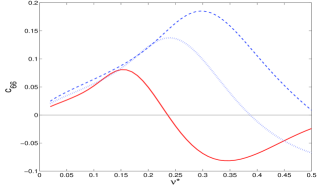
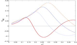
Figure 2: (Color online) Upper panel: shear moduli of the various electronic crystals (in units of $e^{2}/\epsilon\ell$) vs. $\nu^{*}$ in the $n=2$ Landau level. The solid line is for the Wigner crystal, the dotted line is for the 2e BC, and the dashed line is for the 3e BC. Lower panel: same thing for the n=3 level. The dash-dotted line is for the $M=4$ bubble solid.

Figure 2 shows the variation of the shear moduli of various electronic crystals vs. $\nu^{*}$ in the Landau levels $n=2$ and $n=3$. For small values of the partial filling factor $\nu^{*}$, $c_{66}$ is an increasing function of $\nu^{*}$. $c_{66}$ reaches a broad maximum at some characteristic value $\nu^{*}_{m}$, and shows a decreasing behavior for $\nu^{*}>\nu_{m}^{*}$. At some higher value of the partial filling factor $\nu^{*}$, the shear modulus turns negative, indicating an instability of the electronic crystal. Similar results have been obtained by Côté et al.Cote2005 , using a rather sophisticated generalized random phase approximation (GRPA) method. Although the precise location of the maxima of the shear modulus curves is slightly different in their case, the general qualitative behavior of the shear moduli that we find is in good qualitative agreement with the results of Ref. Cote2005, . It is in fact quite remarkable that we were able to reproduce the qualitative behavior of the more involved GRPA method using a simple wavefunction ansatz. This indicates that using single-particle non interacting wavefunctions is a good starting point approximation to study the physics of electronic lattices in quantum Hall systems in higher Landau levels.

The peculiar shape of the shear moduli curves in Fig. 2 suggests that there may be a universal scaling law for the shear modulus, of the form:

$$c_{66}(\nu^{*})=M^{\alpha}f(\nu^{*}/M^{\beta}),$$ (25)

with a universal function $f$ and some scaling exponents $\alpha$ and $\beta$. The identical way in which $c_{66}$ increases at small $\nu^{*}$ for different values of $M$ indicates that $\alpha\simeq\beta$. Figure 3 shows that, at least for the first peak, this is indeed the case, with exponents $\alpha=\beta\simeq 0.68$ for all three values of $M$, $M=1,\,2,$ and $3$.

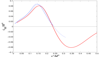
Figure 3: Universal scaling of the shear modulus for the Wigner and bubble crystals in the $n=2$ Landau level. Here the exponent $\alpha\simeq 0.68$.

In Sec. VI, we will use the results of this Section as an input to the variational replica theory of Chitra et al.Chitra2001 and try to analyze the experimental data of Lewis et al.Lewis2004 for the microwave conductivity of the two dimensional electron system in the $n=2$ Landau level. For the moment, we shall turn our attention to the normal modes of the Wigner and bubble crystals in higher Landau levels.

IV Normal modes and zero point energy of the Wigner and bubble crystals

Figure 4: Magnetophonon and magnetoplasmon dispersion curves along the boundary $\Gamma-J-X-\Gamma$ of the irreducible element of the first Brillouin zone for the WC at $\nu^{*}=0.18$ (upper panel) and of the $M=2$ BC at $\nu^{*}=0.25$ (lower panel). Both plots are for the $n=2$ Landau level. Left axes correspond to magnetophonon values and right axes to magnetoplasmon values, and are all measured in units of $\omega_{0}=e^{2}/\epsilon\hbar\ell$.

We now turn our attention to the derivation of the normal modes of the Wigner and bubble crystals. To fix ideas, we shall consider the simplest case of the two-electron bubble crystal in the $n=2$ Landau level, and write for the electron guiding centers ${\bf r}_{mi}$ ($m=0,1$ being the angular momentum quantum number) at a given lattice site ${\bf R}_{i}$ the decomposition ${\bf r}_{mi}={\bf R}_{i}+{\bf u}_{mi}$, where ${\bf u}_{mi}$ is the displacement of the $m$-th electron from the equilibrium lattice position ${\bf R}_{i}$. Expanding the HF energy of a distorted Wigner or bubble crystal

$$E_{HF} = \frac{1}{2}\sum_{\underset{m,m^{\prime}}{i\neq j}}U_{mm^{\prime}}({\bf r}_{mi}-{\bf r}_{m^{\prime}j})$$ (26)

$$+ \sum_{i,m<m^{\prime}}U_{mm^{\prime}}({\bf u}_{mi}-{\bf u}_{m^{\prime}i})$$

to second order in the small displacements ${\bf u}_{mi}$ leads to the elastic energy

$$E_{el}=\frac{1}{2}\sum_{\underset{m,m^{\prime}}{i,j}}u_{m\alpha}({\bf R}_{i})\tilde{\Phi}^{mm^{\prime}}_{\alpha\beta}({\bf R}_{i}-{\bf R}_{j})u_{m^{\prime}\beta}({\bf R}_{j}),$$ (27)

where the generalized elastic matrix $\tilde{\Phi}$ has the following expression

$$\tilde{\Phi}^{mm^{\prime}}_{\alpha\beta}({\bf R}_{i}-{\bf R}_{j}) = \delta_{ij}\delta_{mm^{\prime}}\sum_{k,m^{\prime\prime}}\partial_{\alpha}\partial_{\beta}U_{mm^{\prime\prime}}({\bf R}_{k})$$ (28)

$$- \partial_{\alpha}\partial_{\beta}U_{mm^{\prime}}({\bf R}_{i}-{\bf R}_{j}).$$

Note that, by contrast to the previous Section, where all the electrons within the same bubble were assumed to have the same displacement vector ${\bf u}_{i}$, here we consider the more general case of electrons within the bubble moving independently from one another. This leads to an elastic matrix $\tilde{\Phi}_{\alpha\beta}^{mm^{\prime}}$ which depends on the internal quantum numbers $m,\,m^{\prime}$ of electrons within bubbles. This last elastic matrix is related to the elastic matrix $\Phi_{\alpha\beta}$ of the previous section through the equation:

$$\Phi_{\alpha\beta}=\sum_{m,m^{\prime}}\tilde{\Phi}_{\alpha\beta}^{mm^{\prime}}.$$ (29)

We now are in a position to find the normal modes of the bubble crystal. In the presence of a magnetic field, the equation of motion for the $m$-th electron at lattice site ${\bf R}_{i}$ can be written in the form ($m^{*}$ is the effective mass of the electron in the host semiconductor and $\varepsilon_{\alpha\beta}$ is the totally antisymmetric tensor in two dimensions)

$$m^{*}\frac{d^{2}}{dt^{2}}u_{m\alpha}({\bf R}_{i}) = -\sum_{j,m^{\prime}}\tilde{\Phi}_{\alpha\beta}^{mm^{\prime}}({\bf R}_{i}-{\bf R}_{j})u_{m^{\prime}\beta}({\bf R}_{j})$$ (30)

$$- \frac{eB}{c}\varepsilon_{\alpha\beta}\frac{d}{dt}u_{m\beta}({\bf R}_{i}).$$

We shall seek a solution to the above equation of motion that represents a wave with angular frequency $\omega$ and wavevector ${\bf q}$, i.e. $u_{m\alpha}({\bf R}_{i})=A_{m\alpha}({\bf q})e^{i({\bf q}\cdot{\bf R}_{i}-\omega t)},$ where the ${\bf A}_{m}$’s are complex coefficients whose ratios specify the relative amplitude and phase of the vibrations of the electrons within each primitive cell. Substituting the above expression into Eq. (30) results in the following secular equation for the Wigner crystal:

$$\begin{pmatrix}\tilde{\Phi}_{xx}^{00}({\bf q})-\omega^{2}&\tilde{\Phi}_{xy}^{00}({\bf q})-i\omega\omega_{c}\\ \tilde{\Phi}_{xy}^{00}({\bf q})+i\omega\omega_{c}&\tilde{\Phi}_{yy}^{00}({\bf q})-\omega^{2}\end{pmatrix}\begin{pmatrix}A_{0x}\\ A_{0y}\end{pmatrix}=0,$$ (31)

while for the $M=2$ bubble solid the secular equation is given by

$$\begin{pmatrix}\tilde{\Phi}_{xx}^{00}({\bf q})-\omega^{2}&\tilde{\Phi}_{xx}^{01}({\bf q})&\tilde{\Phi}_{xy}^{00}({\bf q})-i\omega\omega_{c}&\tilde{\Phi}_{xy}^{01}({\bf q})\\ \tilde{\Phi}_{xx}^{01}({\bf q})&\tilde{\Phi}_{xx}^{11}({\bf q})-\omega^{2}&\tilde{\Phi}_{xy}^{01}({\bf q})&\tilde{\Phi}_{xy}^{11}({\bf q})-i\omega\omega_{c}\\ \tilde{\Phi}_{xy}^{00}({\bf q})+i\omega\omega_{c}&\tilde{\Phi}_{xy}^{01}({\bf q})&\tilde{\Phi}_{yy}^{00}({\bf q})-\omega^{2}&\tilde{\Phi}_{yy}^{01}({\bf q})\\ \tilde{\Phi}_{xy}^{01}({\bf q})&\tilde{\Phi}_{xy}^{11}({\bf q})+i\omega\omega_{c}&\tilde{\Phi}_{yy}^{01}({\bf q})&\tilde{\Phi}_{yy}^{11}({\bf q})-\omega^{2}\end{pmatrix}\begin{pmatrix}A_{0x}\\ A_{1x}\\ A_{0y}\\ A_{1y}\end{pmatrix}=0\,,$$ (32)

where we defined

$$\tilde{\Phi}_{\alpha\beta}^{mm^{\prime}}({\bf q})=\frac{1}{m^{*}}\sum_{i}\tilde{\Phi}_{\alpha\beta}^{mm^{\prime}}({\bf r})e^{-i{\bf q}\cdot{\bf R}_{i}},$$ (33)

and used the fact that $\tilde{\Phi}_{\alpha\beta}^{mm^{\prime}}({\bf q})=\tilde{\Phi}_{\beta\alpha}^{mm^{\prime}}({\bf q})=\tilde{\Phi}_{\alpha\beta}^{m^{\prime}m}({\bf q})$.

The above secular equations have a non-vanishing solution (for the ${\bf A}_{m\alpha}$’s) only if the determinant of the secular matrix is zero. This leads to two types of solutions for the eigenmodes:Cote1990 magnetophonon modes, with eigenfrequencies which vanish like $q^{3/2}$ as $q\to 0$, and magnetoplasmon modes which tend to a finite limit as $q\to 0$. In Fig. 4 we show our solution for the magnetophonon and magnetoplasmon modes of the WC and the $M=2$ BC in the $n=2$ Landau level. As is expected, the eigenmode spectrum for the $2e$ BC has four branches (compared to two for the WC). We note that the magnetophonon dispersion curves we obtain are identical to the ones obtained by Côté et al.Cote2003 within the time-dependent HF approach. To our knowledge, however, the magnetoplasmon modes of electronic crystals, shown here in Fig. 4, have not been previously studied in higher LLs.

We now turn our attention to the calculation of the zero point energy of the Wigner and bubble crystals. To this end, we shall use the approach of Cunningham,Cunningham1974 whereby one evaluates the energy of the magnetophonon and magnetoplasmon modes at a given number $N_{p}$ of predefined points ${\bf q}_{i}$ within the irreducible element of the first Brillouin zone for the triangular lattice, with appropriate weights $\alpha_{i}$ assigned to each one of these points. The zero-point energy (per electron) for the $M$-electron BC, in units of $e^{2}/\epsilon\ell$, is then given by

$$E_{ZP}=\frac{1}{2M\omega_{0}}\sum_{j=1}^{2M}\sum_{i=1}^{N_{p}}\alpha_{i}\omega_{j}({\bf q}_{i}),$$ (34)

where $\omega_{0}=e^{2}/\epsilon\hbar\ell$. The resulting zero-point energies for $N_{p}=6$ (using the special points and associated weightsRemark1 given in Ref. Cunningham1974, ) are shown for a range of partial filling factor values in Table. 1. We notice that for $\nu^{*}\leq 0.20$ the zero-point energy of the WC always exceeds the corresponding quantity for the two-electron BC, which suggests that quantum fluctuations will shift the transitional filling factor $\nu^{*}_{1,2}$ between the WC and the 2e BC toward smaller values. However, this shift in the transitional values of $\nu^{*}$, of order 0.02, is rather small, and has no substantial effect on the overall phase diagram of the 2DES in higher LLs.

$\nu^{*}$	$E_{WC}$	$E_{2eBC}$
0.05	0.362825	0.360756
0.10	0.368391	0.360716
0.15	0.379527	0.362053
0.20	0.382453	0.365264
0.25	0.367643	0.368439

Table 1: Zero point energy (per particle) of the WC and 2e BC for different partial filling factor values $\nu^{*}$. Energy is measured in units of $e^{2}/\epsilon\ell$.

V Effect of finite sample thickness and of lower Landau levels

Let us now investigate the effect of finite sample thickness and of lower Landau levels on the energetics of the Wigner and bubble crystals in higher LLs. To this end, we shall replace the bare Coulomb potential in Eqs. (4a)-(4b) with the following effective interaction

$$v(q)=\frac{2\pi e^{2}}{\varepsilon(q)q}e^{-\lambda q\ell}.$$ (35)

The parameter $\lambda$ models a finite thickness sample, and is generally taken to be of order unity.Zhang1986 The effect of lower LLs is encoded in the wavevector-dependent dielectric constant $\varepsilon(q)$, for which we shall use the following expression, due to Aleiner and GlazmanAleiner1995

$$\varepsilon(q)=\epsilon\Big{\{}1+\frac{2}{qa_{B}}[1-J_{0}^{2}(qR_{c})]\Big{\}},$$ (36)

with $a_{B}=\hbar^{2}\epsilon/m^{*}e^{2}$ the effective Bohr radius and $R_{c}=\sqrt{2n+1}\ell$.

The form of the effective Coulomb interaction of Eq. (35) makes it difficult to find an analytic expression for the Fock part of the interaction potential, Eq. (4b). To evaluate the cohesive energy, the ${\bf q}$ integration in this last equation is performed numerically. In Figs. (5) and (6), we plot the cohesive energies of the Wigner crystal, bubble phases and stripe states in the second ($n=2$) and third ($n=3$) Landau levels, respectively. In each of these two figures, the upper panel corresponds to $\lambda=0$, while the lower panel corresponds to $\lambda=1$. The screening by lower LLs has the most drastic effect on the cohesive energy, shifting it upwards by about $50$ percent of its bare value, and finite sample thickness also tends to shift the cohesive energies up, although in a less pronounced fashion. It is noteworthy that these shifts in the cohesive energy curves do not alter the overall phase diagram. As can be seen from Fig. 5, the transitional values $\nu^{*}_{1,2}$ from WC to the 2e bubble phase, and $\nu^{*}_{2,3}$ from $M=2$ to $M=3$, are slightly shifted downwards by screening alone (we find $\nu^{*}_{1,2}\simeq 0.2$ and $\nu^{*}_{1,2}\simeq 0.35$ with screening, while $\nu^{*}_{1,2}\simeq 0.22$ and $\nu^{*}_{2,3}\simeq 0.37$ without screening). Finite thickness effects on the other hand shift transitional filling factors upwards, restoring them to values that are very close to their bare values. In all cases, these shifts do not affect the overall phase diagram, which remains the same as in the ideal case of zero sample thickness and no screening by lower Landau levels.

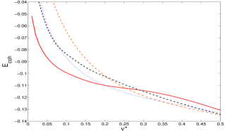
Figure 5: (Color online) Cohesive energies of the Wigner and bubble crystals in the $n=2$ LL in units of $e^{2}/\epsilon\ell$, with the interaction potential $V_{HF}$ resulting from the effective Coulomb potential in Eq. (35). The solid line is for the Wigner crystal, the dotted line is for the two-electron bubble phase, the dash-dotted line is for the $M=3$ BC, and the dashed line is for the stripe phase. The upper panel is for $\lambda=0$, and the lower panel is for $\lambda=1$.

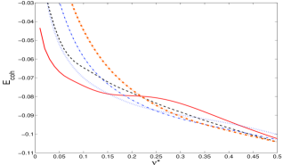
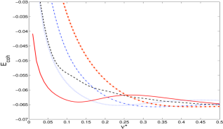
Figure 6: (Color online) Same as in Fig. 5, but for Landau level $n=3$. The thick dash-dotted line is for the bubble state with $M=4$.

We have also calculated the shear moduli of the Wigner and bubble crystals in presence of screening and taking finite thickness effects into account. As we mentioned above, in the presence of screening, it becomes difficult to obtain an analytic expression for the Fock part of the HF interaction potential, and the method of Sec. III.2 becomes impractical. A more efficient way to extract the elastic coefficients of that case consists in finding the cohesive energy of a distorted crystal for a given uniform deformation. The elastic energy will then be given by the excess energy of the deformed crystal with respect to the reference undistorted state. For two-dimensional uniform deformations, such that the displacement vector ${\bf u}({\bf r})$ is given by

$$u_{\alpha}=u_{\alpha,\beta}x_{\beta}\,,$$ (37)

with constant coefficients $u_{\alpha,\beta}$, it can be shownMiranovic2001 that the reciprocal lattice also experiences a homogeneous deformation, with the deformed reciprocal lattice vectors $\{{\tilde{\bf Q}}\}$ given in terms of the original ones $\{{\bf Q}\}$, to first order in the small displacements $\{u\}$, by:

$$\tilde{Q}_{\alpha}=Q_{\alpha}-u_{\beta,\alpha}Q_{\beta}.$$ (38)

To find a given elastic modulus, we calculate the HF energy of the corresponding distorted state (with distortion amplitude $u_{0}$), and extract the elastic constant from the excess energy $E_{HF}(u_{0})-E_{HF}(0)$. For example, to extract the shear modulus $c_{66}$ we calculate the HF energy $E_{HF}(u_{0})$ of the distorted crystal using the following reciprocal lattice vectors:

$$\tilde{Q}_{x} = Q_{x}-u_{0}Q_{y}\,,$$ (39a)

$$\tilde{Q}_{y} = Q_{y}\,,$$ (39b)

corresponding to the shear deformation polarized along $y$ such that ${\bf u}({\bf r})=u_{0}\,x\,\hat{\bf y}$. The shear modulus (in units of energy/particle) is then given by:

$$c_{66}=\frac{2}{u_{0}^{2}}\,\big{[}E_{HF}(u_{0})-E_{HF}(0)\big{]}.$$ (40)

Note that this procedure allows us to extract the elastic moduli without Taylor expanding in the small displacement vectors $\{{\bf u}\}$, which allows us to better handle anharmonic effects which might be important in case quantum fluctuations happen to be largeFisher1982 ; Cote1990 (which might be the case with the softer lattices in presence of screening by lower LLs). Note also that, since cohesive energy calculations involve reciprocal lattice sums that avoid summing over the (diverging) contribution of the ${\bf Q}=0$ Hartree term, one should add to the results for the compression modulus $c_{11}$ obtained by the above method a term $\frac{1}{A_{c}}U_{H}(q)$ to obtain the correct compression moduli of the electronic solid.

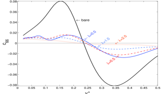
Figure 7: (Color online) Upper panel: Shear moduli (in units of $e^{2}/\epsilon\ell$) for the WC (solid lines) in the $n=2$ LL with the interaction potential $V_{HF}$ resulting from the effective Coulomb potential in Eq. (35). The succession of curves is for $\lambda=0,\,0.5,\,1$ and $2$. Lower panel: shear moduli of the WC and for the 2 and 3 electron bubble solids (from bottom to top) in presence of screening by lower LLs and with $\lambda=1$.

In order to test the validity of the above procedure, we have calculated the shear moduli of the Wigner and $M=2$ bubble crystals in the $n=2$ Landau level. As can be seen in Fig. 7 (upper panel), we obtain the same shear modulus for the WC as in Sec. III.2 where we used a Taylor expansion of the interaction energy in the small displacements $\{{\bf u}({\bf r})\}$, which is a consistency check on our calculations. In Fig. 7, we also show the results we obtain for the shear modulus of the WC in presence of screening and for various values of the parameter $\lambda$. It is seen that screening by lower LLs alone (i.e., with $\lambda=0$) considerably softens the shear modulus with respect to the unscreened case, and higher values of $\lambda$ lead to even smaller values of the shear modulus of the WC. In the lower panel of Fig. 7, we plot the shear moduli of the WC and of the 2 and 3 electron bubble states in the $n=2$ LL in presence of screening and using $\lambda=1$. As it can be seen, the shear moduli of these various types of crystals are affected by the screening of the Coulomb interaction between electrons in similar but nonequivalent ways, with the strongest effect impacting the WC. This is quite understandable, given that a shear deformation of a BC does not affect the part of the cohesive energy coming from electrons inside the bubbles. It is to be noted also that the universal scaling of Eq. (25) holds only approximatively in the screened case, as shown in Fig. 8, where we used $\alpha=\beta\simeq 0.75$. We shall discuss some of the implications of our results in Sec. VI.

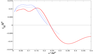
Figure 8: Universal scaling of the shear modulus for the Wigner and bubble crystals in the $n=2$ Landau level in presence of screening and finite thickness effects. Here we used the value $\lambda=1$ for the screening strength, and the value $\alpha\simeq 0.75$ for the scaling exponent.

VI Link with experiment: Consequence for the microwave conductivity of two dimensional bubble crystals

We now would like to discuss the experimental implications of our results. Our investigation of the dynamics of bubble solids stemmed primarily from a desire to understand recent microwave conductivity experiments by Lewis et al.Lewis2004 in the second ($n=2$) Landau level, where the appearance of a second resonance peak around $\nu^{*}\sim 0.16$ was attributed to the formation of a bubble phase, which coexists with a Wigner crystal over a range of values of $\nu^{*}$. In what follows, we shall attempt a qualitative analysis of the experimental results of Lewis et al.Lewis2004 in light of the results of the elasticity theory presented in this paper combined with the theoretical predictions of Refs. Fogler2000, ; Chitra2001, .

According to Chitra et al.,Chitra2001 the resonance frequency due to pinning of a two dimensional Wigner crystal in a strong magnetic field is given by

$$\omega_{p}\simeq\frac{\Sigma}{\rho_{m}\omega_{c}},$$ (41)

where $\rho_{m}=m/({\pi}a^{2})$ is the mass density, $\omega_{c}=eB/m$ is the cyclotron frequency, and where $\Sigma$ is given by (we neglect an overall numerical constant of order unity):

$$\Sigma\simeq\frac{c_{66}}{R_{a}^{2}}\big{(}\frac{a}{\xi_{0}}\big{)}^{6}.$$ (42)

In the above expression, $\xi_{0}$ is the greatest of $\ell$ and the correlation length $\xi_{d}$ of the disorder potential. On the other hand, $R_{a}$ is the length scale at which electron displacements become of order $a$, and is given by (here $\Delta$ is the variance of the random pinning potential, whose distribution was assumed by Chitra et al. to be Gaussian and of short range):

$$R_{a}=\frac{\pi c_{66}a^{4}}{\sqrt{\Delta}}.$$ (43)

Using Eq. (43) into Eq. (42), we obtain:

$$\Sigma\sim\frac{\Delta}{c_{66}\xi_{0}^{6}a^{2}},$$ (44)

and hence

$$\omega_{p}\simeq\frac{\Delta}{\rho_{m}\omega_{c}c_{66}\xi_{0}^{6}a^{2}}.$$ (45)

Using the fact that $\rho_{m}=m/\pi a^{2}$, we see that $\rho_{m}a^{2}=m$, and hence:

$$\omega_{p}(\nu^{*})\sim\frac{\Delta}{m\omega_{c}\xi_{0}^{6}c_{66}}.$$ (46)

In the above equation, $m$ is the mass of electrons within a unit lattice cell, and hence $m=Mm^{*}$, where $m^{*}$ is the effective electron mass in the host semiconductor. We thus obtain:

$$\omega_{p}(\nu^{*})\sim\frac{\Delta}{Mm^{*}\omega_{c}\xi_{0}^{6}c_{66}}.$$ (47)

The above result implies that the $\nu^{*}$ dependence of the resonance frequency $\omega_{p}$ arises mainly from the dependence of the effective shear modulus $c_{66}$ on the partial filling factor $\nu^{*}$ (the dependence of $\xi_{0}$ and $\omega_{c}$ on $\nu^{*}$ being rather weak in Landau levels of index $n\geq 2$). We thus see that knowledge of the variation of $c_{66}$ vs. $\nu^{*}$ in a given Landau level and for a given bubble crystal should allow us to easily infer the variation of $\omega_{p}$ vs. $\nu^{*}$. Conversely, analysis of experimental data of $\omega_{p}$ vs. $\nu^{*}$ using the above expression (and our Hartree-Fock results for $c_{66}(\nu^{*})$) should allow us to identify Wigner crystal and bubble phases, and transitions between these phases.

We now turn our attention to the experimental results of Ref. Lewis2004, , and more specifically to Fig. 3 in this last reference, where the authors plot experimental resonance frequencies of the two-dimensional electron system in the $n=2$ Landau level as a function of the filling factor $\nu$. At small $\nu^{*}$, there is only one resonance peak, whose frequency decreases with increasing $\nu^{*}$, with a minimum around $\nu^{*}\simeq 0.19$. The frequency of the above peak then slightly increases, until the peak disappears around $\nu^{*}\simeq 0.27$. This behavior is in qualitative agreement with the behavior of a Wigner crystal if we use our shear modulus of Fig. 2 (Wigner crystal in the $n=2$ LL) in conjunction with Eq. (47).

Figure 3 of Lewis et al. also shows the peak frequency of a second resonance peak which appears at $\nu^{*}\geq 0.16$. The $\nu^{*}$ dependence of the frequency of this second resonance peak, however, does not seem to be fully consistent with Eq. (47) above and with the shear moduli of the $M=2$ bubble phase plotted in Fig. 2. Indeed, in the range $0.23\leq\nu^{*}\leq 0.35$, from the decreasing behavior of the shear modulus of the bubble phase in Fig. 2, we expect an increasing behavior of the peak frequency $\omega_{p}$ vs. $\nu^{*}$. The experimental result of Ref. Lewis2004, show a decreasing peak frequency in this range of filling factors, in disagreement with the theoretical considerations above. Equally important is the fact that Eq. (47) predicts a factor of $1/M$ difference between the frequencies of different bubble states, while experimentally it seems that a factor $1/\sqrt{M}$ is observed instead.

It is to be noted that, in their recent replica study of bubble phases pinned by random disorder, the authors of Ref. Cote2005, claim to have been able to successfully describe the $\nu^{*}$ dependence of the resonance peak of both Wigner and bubble crystals, except on the region between $\nu^{*}=0.16$ and $\nu^{*}=0.28$ where the two phases are assumed to coexist. We therefore may speculate that the disagreement we find in the present study may be due to a possible breakdown of Eq. (41), which in fact is derived by Chitra et al.Chitra2001 by linearizing nonlinear self-consistent replica calculation, and that a careful and exhaustive treatment such as the one in Ref. Cote2005, , where the full nonlinear replica equations are numerically solved in a self-consistent way, can lead to better agreement between theoretical predictions and experimental observations.

We now briefly comment on the effect of screening by lower LLs and of finite sample thickness (as modeled by the parameter $\lambda$ of the Zhang-Das Sarma potential of the previous Section) on the microwave response. Since we have shown that both effects tend to reduce the shear modulus with respect to the bare case, we conclude that the resonance peak will tend to shift toward higher frequencies as the sample thickness or Landau level index is increased, an effect that may be testable experimentally. More importantly, in presence of screening and for finite thickness samples, we find that there is a finite gap between the shear moduli of the Wigner and bubble crystals, and that gap might accentuate the finite gap observed in the coexistence region between the pinning frequencies of the Wigner and the 2e bubble crystals, making it more pronounced. Lewis2004 In fact, it would be interesting to do a full self-consistent calculation, like the one done in ref. Cote2005, , in presence of screening and finite thickness effects, and see whether the experimentally observed gap between the pinning frequencies in the coexistence region can be reproduced theoretically.

VII Conclusions

In conclusion, in this paper we have calculated the cohesive energies, shear moduli, and normal (magnetophonon and magnetoplasmon) modes of the Wigner and bubble crystals in higher LLs. Going beyond previous treatments, we have studied the effects of screening by lower Landau levels as well as the case of finite sample thickness. We found that both effects reduce the cohesive energies and elastic moduli, with the screening by lower Landau levels having the most pronounced effect. The transitional values of the filling factor as well as the overall nature of the phase diagram remain, however, unchanged by both effects. We have also examined the electromagnetic response of the Wigner and bubble crystals, and have noticed that, while the $\nu^{*}$ dependence of the shear modulus of the WC, when used in standard theories of the electromagnetic response of electronic crystals, is in good qualitative agreement with experimental data, the shear modulus of the 2e BC has a $\nu^{*}$ dependence which, in contrast, is in disagreement with the experimentally observed behavior. This led us to suggest that a full numerical solution of the non-linear self-consistent replica equationsCote2005 may be needed in order to understand the electromagnetic response of bubble crystals, by contrast to Wigner crystals for which a linearized estimateChitra2001 of the resonance frequency may be adequate.

Before closing, we briefly comment on an issue that has not been previously addressed in the literature, and that is the issue of gauge invariance. In principle, all physical observables are gauge-independent. However, HF being an approximate (i.e. not an exact) theory, different HF derivations done in different gauges will not necessarily give the same results. As a check to our calculations of the cohesive energies of the Wigner and bubble crystals, and to make sure that the same qualitative phase diagram that we obtained above in the Landau gauge is not affected by a different choice of gauge, we have rederived the HF interaction potentials and the phase diagram of the 2D electron system in the symmetric gauge, using a HF approach similar to the one used a long time ago by Maki and ZotosMaki1983 to study the properties of the two-dimensional Wigner crystal in the lowest Landau level. In Appendix C, we derive expressions for the interaction potential $U_{mm^{\prime}}(r)$ between electrons of angular momenta $m$ and $m^{\prime}$, with $m,m^{\prime}=0,1,2$ by finding the average Coulomb energy between symmetric-gauge electronic wavefunctions in the $n=2$ Landau level. These interaction potentials have the same qualitative behavior as the potentials derived within the Landau gauge HF approach of the text, and lead to very similar cohesive energies as the ones predicted above, although with slightly different numerics.

Appendix A Projected densities and HF potentials

In order for our paper to be self-contained, in this Appendix we give the explicit expressions of the projected densities and Hartree-Fock potentials that we used in deriving our cohesive energies. From the usual expressions of the noninteracting wavefunctions $\varphi_{nm}({\bf r})$ (see Eq. (54), and the definitions (2)-(6), we obtain that the projected densities $\tilde{\rho}_{0}({\bf q})$ and $\tilde{\rho}_{1}({\bf q})$ are given, both in $n=2$ and $n=3$, by (throughout this Appendix, $q$ stands for the dimensionless quantity $q\ell$)

$$\tilde{\rho}_{0}({\bf q})=e^{-q^{2}/4},$$ (48a)

$$\tilde{\rho}_{1}({\bf q})=(1-\frac{1}{2}q^{2})e^{-q^{2}/4}.$$ (48b)

On the other hand, performing the integrals in Eqs. (4a)-(4b), we obtain the following Hartree and Fock potentials in LL $n=2$:

$$V_{H}(q) =\Big{(}\frac{2\pi e^{2}\ell}{\epsilon}\Big{)}\frac{e^{-q^{2}/2}}{64q}\big{(}8-8q^{2}+q^{4}\big{)}^{2},$$ (49a)

$$V_{F}(q) =-\Big{(}\frac{2\pi e^{2}\ell}{\epsilon}\Big{)}\frac{e^{-q^{2}/4}}{128}\sqrt{\frac{\pi}{2}}\Big{[}(82-52q^{2}+44q^{4}-10q^{6}+q^{8}\big{)}\mbox{I}_{0}(\frac{q^{2}}{4})-q^{4}\big{(}30-8q^{2}+q^{4}\big{)}\mbox{I}_{1}(\frac{q^{2}}{4})\Big{]},$$ (49b)

while for LL $n=3$ the Hartree and Fock potentials are given by:

$$V_{H}({\bf q}) =\Big{(}\frac{2\pi e^{2}\ell}{\epsilon}\Big{)}\,\frac{e^{-q^{2}/2}}{2304q}\big{(}48-72q^{2}+18q^{4}-q^{6}\big{)}^{2},$$ (50a)

$$V_{F}({\bf q}) =-\Big{(}\frac{2\pi e^{2}\ell}{\epsilon}\Big{)}\frac{e^{-q^{2}/4}}{4608}\sqrt{\frac{\pi}{2}}\Big{[}\big{(}2646-2430q^{2}+2889q^{4}-1236q^{6}+270q^{8}-26q^{10}+q^{12}\big{)}\mbox{I}_{0}(\frac{q^{2}}{4})$$

$$-q^{4}\big{(}1539-828q^{2}+224q^{4}-24q^{6}+q^{8}\big{)}\mbox{I}_{1}(\frac{q^{2}}{4})\Big{]}.$$ (50b)

Appendix B Cohesive energy of the stripe phase

For completeness, in this Appendix, we briefly review the cohesive energy of the stripe phase of the two-dimensional electron system. Following Fogler et al.Fogler1996 and Goerbig et al.Goerbig2004 , we write the cohesive energy per particle $E_{coh}$ in the form

$$E_{coh}=\frac{n_{B}}{2\nu^{*}}\sum_{\bf q}V_{HF}(q)|\Delta(q)|^{2}$$ (51)

where $n_{B}=1/(2\pi\ell^{2})$ is the flux density, and where $\Delta({\bf q})=\rho({\bf q})/(n_{B}A)$ is the Fourier transform of the local guiding center filling factor $\nu^{*}({\bf r})$ ($A$ is the area of the sample). For a stripe state, $\nu^{*}({\bf r})=\sum_{i}\Theta(|x-x_{i}|-a/2)$, with $a$ the width of a given stripe, and $x_{i}$ the location of the center of the $i$-th stripe. If we denote by $L_{s}$ the stripe periodicity (such that $x_{i}=iL_{s}$), and note thatFogler1996 ; Goerbig2004 $\nu^{*}=a/L_{s}$, then we obtain after a few manipulations that the cohesive energy per particle of Eq. (51) is given by

$$E_{coh}=\frac{n_{B}}{2\pi^{2}\nu^{*}}{\sum_{n}}^{\prime}V_{HF}\Bigg{(}\frac{2\pi n}{L_{s}}\Bigg{)}\frac{\sin^{2}(\pi\nu^{*}n)}{n^{2}},$$ (52)

where the prime on the sum sign indicates that the (diverging) Hartree contribution for $n=0$ is excluded from the summation (the $n=0$ Fock term being included). The above expression is then minimized with respect to $L_{s}$, with the optimal stripe periodicity foundGoerbig2004 to be approximately given by $L_{s}^{*}\simeq 2.76\ell\sqrt{2n+1}$ in $n=2$ and $L_{s}^{*}\simeq 2.74\ell\sqrt{2n+1}$ in $n=3$. The cohesive energy in the stripe phase is then given by the optimal value $E_{coh}(L_{s}^{*})$.

Appendix C Gauge dependence of the cohesive energies: Hartree-Fock approach in the symmetric gauge

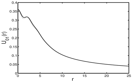
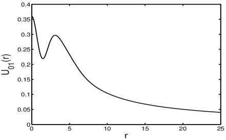
Figure 9: Upper panel: Interaction potential $U_{01}(r)$ (in units of $e^{2}/\ell$) vs. $r$ (in units of $\ell$) as obtained from the HF approach in the symmetric gauge, Eqs. (64e)-(64f), in the $n=2$ Landau level. The dotted line corresponds to the numerator $N_{01}(r)$ alone. Lower panel: Effective interaction potential $U_{01}(r)$ in the Landau gauge.

Figure 10: Interaction potential $U_{00}$ (in units of $e^{2}/\ell$) vs. $r$ (in units of $\ell$) in the $n=2$ Landau level. The solid line is the Landau gauge result, while the dashed line is the result for $N_{00}(r)$ in the symmetric gauge, Eq. (64a). The dotted line is the whole function $U_{00}(r)=N_{00}(r)/D_{00}(r)$. (Note that this last function has no physical meaning at small separations, i.e. for $r\leq\ell$, due to the Pauli exclusion principle for Fermions.)

In this Appendix, we want to confirm the qualitative features of the phase diagram of electrons in higher LLs derived in the text using a different gauge for the applied magnetic field, namely the symmetric gauge ${\bf A}=\frac{B}{2}(-y\hat{\bf x}+x\hat{\bf y})$. To this end, we shall use a HF approach which is similar in spirit to the approach of Maki and ZotosMaki1983 to derive the effective interaction potentials $U_{mm^{\prime}}(r)$ in the second ($n=2$) Landau level. Let us consider two electrons with angular momenta $m_{1}$ and $m_{2}$ and with guiding centers located at lattice sites ${\bf R}_{1}$ and ${\bf R}_{2}$, respectively. We shall use for the wave function of the two-bubble system the following antisymmetric combination

$$\Psi({\bf r}_{1},{\bf r}_{2}) = \frac{1}{\sqrt{2}}\big{(}\varphi_{nm_{1}{\bf R}_{1}}({\bf r}_{1})\varphi_{nm_{2}{\bf R}_{2}}({\bf r}_{2})$$ (53)

$$- \varphi_{nm_{1}{\bf R}_{1}}({\bf r}_{2})\varphi_{nm_{2}{\bf R}_{2}}({\bf r}_{1})\big{)},$$

where $\varphi_{nm{\bf R}}({\bf r})$ is the symmetric gauge wavefunction with angular momentum $m$ which is located around the lattice site ${\bf R}_{k}$, $\varphi_{nm\bf R}({\bf r})=\varphi_{nm}({\bf r}-{\bf R})$, with

$$\varphi_{nm}({\bf r}) = C_{nm}\big{(}\frac{r}{\ell}\big{)}^{|n-m|}e^{i(n-m)\theta}e^{-r^{2}/4\ell^{2}}$$ (54)

$$\times L^{|n-m|}_{(n+m-|n-m|)/2}\big{(}\frac{r^{2}}{2\ell^{2}}\big{)},$$

where we denote by $\theta$ the polar angle of vector ${\bf r}$, i.e. ${\bf r}=(r\cos\theta,r\sin\theta)$, and where the normalization constant $C_{nm}$ is given by:

$$C_{nm}=\frac{1}{\ell}\begin{cases}\sqrt{\frac{2^{n-m}n!}{2\pi m!}}&\mbox{if $m\geq n$,}\\ {}&{}\textstyle\\ \sqrt{\frac{2^{m-n}m!}{2\pi n!}}&\mbox{if $n\geq m$.}\end{cases}$$ (55)

The average potential energy for this state is given by (we here for simplicity set $\epsilon=1$):

$$U_{m_{1}m_{2}}({\bf R}_{1},{\bf R}_{2})=\frac{\langle\Psi|\frac{e^{2}}{|{\bf r}_{1}-{\bf r}_{2}|}|\Psi\rangle}{\langle\Psi|\Psi\rangle}.$$ (56)

Note that the above expression is valid for arbitrary ${\bf R}_{1}$ and ${\bf R}_{2}$ only if $m_{1}\neq m_{2}$. In the special case $m_{1}=m_{2}$, because of the Pauli exclusion principle for Fermions the above expression for $U_{m_{1}m_{2}}$ only makes sense at separations $|{\bf R}_{1}-{\bf R}_{2}|$ larger than the typical extension of the wavefunctions $\varphi_{nm}({\bf r})$, which is of order $\ell$.

Now, the numerator of the above expression is given by (to simplify the notation, in the rest of this Appendix we shall drop the LL index $n$ from the $\varphi_{nm}$ wavefunctions):

$$N_{m_{1},m_{2}}({\bf R}_{1},{\bf R}_{2})=e^{2}\int\frac{d{\bf r}_{1}d{\bf r}_{2}}{|{\bf r}_{1}-{\bf r}_{2}|}\big{[}|\varphi_{m_{1},{\bf R}_{1}}({\bf r}_{1})|^{2}|\varphi_{m_{2},{\bf R}_{2}}({\bf r}_{2})|^{2}-\varphi_{m_{1},{\bf R}_{1}}^{*}({\bf r}_{1})\varphi_{m_{2},{\bf R}_{2}}^{*}({\bf r}_{2})\varphi_{m_{2},{\bf R}_{2}}({\bf r}_{1})\varphi_{m_{1},{\bf R}_{1}}({\bf r}_{2})\big{]}.$$ (57)

The denominator on the other hand is given by

$$D_{m_{1},m_{2}}({\bf R}_{1},{\bf R}_{2})=1-\int d{\bf r}_{1}d{\bf r}_{2}\varphi_{m_{1},{\bf R}_{1}}({\bf r}_{1})\varphi_{m_{1},{\bf R}_{1}}^{*}({\bf r}_{2})\varphi_{m_{2},{\bf R}_{2}}({\bf r}_{2})\varphi_{m_{2},{\bf R}_{2}}^{*}({\bf r}_{1})=1-\big{|}\int d{\bf r}_{1}\varphi_{m_{1},{\bf R}_{i}}({\bf r}_{1})\varphi_{m_{2},{\bf R}_{j}}^{*}({\bf r}_{1})\big{|}^{2}.$$ (58)

Now, using the fact that

$$\varphi_{m\bf R}({\bf r})=\varphi_{m}({\bf r}-{\bf R})=\int_{\bf q}\varphi_{m}({\bf q})e^{-i{\bf q}\cdot({\bf r}-{\bf R})},$$ (59)

one can show, after a few manipulations, that the Hartree part of $$N_{m_{1}m_{2}}$$ is given by

$$N_{m_{1}m_{2}}^{H}({\bf R}_{i},{\bf R}_{j})=\int_{\bf q}\frac{2\pi e^{2}}{q}\big{(}\int d{\bf r}_{1}|\varphi_{m_{1}}({\bf r}_{1})|^{2}e^{i{\bf q}\cdot{\bf r}_{1}}\big{)}\big{(}\int d{\bf r}_{2}|\varphi_{m_{2}}({\bf r}_{2})|^{2}e^{-i{\bf q}\cdot{\bf r}_{2}}\big{)}e^{i{\bf q}\cdot({\bf R}_{i}-{\bf R}_{j})}.$$ (60)

Similarly, the Fock part of $$N_{m_{1}m_{2}}$$ can be written in the form

$$N_{m_{1}m_{2}}^{F}({\bf R}_{i},{\bf R}_{j})=-\int_{\bf q}\frac{2\pi e^{2}}{q}\big{|}\int d{\bf r}\varphi_{m_{1}}^{*}({\bf r})\varphi_{m_{2}}({\bf r}+{\bf R}_{i}-{\bf R}_{j})e^{i{\bf q}\cdot{\bf r}}\big{|}^{2}.$$ (61)

Finally, the denominator $D_{m_{1}m_{2}}$ can also be written in the form

$$D_{m_{1}m_{2}}({\bf R}_{i},{\bf R}_{j})=1-\big{|}\int d{\bf r}\varphi_{m_{1}}^{*}({\bf r})\varphi_{m_{2}}({\bf r}+{\bf R}_{i}-{\bf R}_{j})\big{|}^{2}.$$ (62)

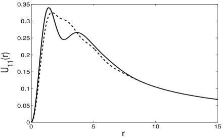
Figure 11: Interaction potential $U_{11}$ (in units of $e^{2}/\ell$) vs. $r$ (in units of $\ell$) in the $n=2$ Landau level. The solid line is the Landau gauge result, while the dotted line is the symmetric gauge result for $N_{11}(r)$, Eq. (64c).

Eqs. (60)-(62) show that both Hartree and Fock parts of $N_{m_{1}m_{2}}$ as well as the denominator $D_{m_{1}m_{2}}$ depend only on the difference ${\bf R}_{i}-{\bf R}_{j}$ and are thus translationally invariant as they should be. Using for the $\varphi_{m,{\bf R}}$’s the wavefunctions for noninteracting electrons in the $n$-th LL, Eq. (54), and performing the integrations in Eqs. (60)-(62) (which is most efficiently done in cartesian coordinates), we obtain that the above potential energy, Eq. (56), can be written in the form:

$$U_{m_{1}m_{2}}({\bf R}_{1}-{\bf R}_{2})=\frac{e^{2}}{\ell}\frac{N_{m_{1}m_{2}}({\bf R}_{1}-{\bf R}_{2})}{D_{m_{1}m_{2}}({\bf R}_{1}-{\bf R}_{2})}$$ (63)

where the functions $N_{m_{1}m_{2}}$ and $D_{m_{1}m_{2}}$ are given, for $n=2$ and $m_{1},m_{2}=0,1$, by ($\mbox{I}_{0}$ and $\mbox{I}_{1}$ are modified Bessel functions)

$$N_{00}(r)=-\frac{\sqrt{\pi}e^{-\frac{r^{2}}{4}}}{32768}\big{(}9360-2944r^{2}+560r^{4}-32r^{6}+r^{8}\big{)}$$

$$+\frac{\sqrt{\pi}e^{-\frac{r^{2}}{8}}}{65536}\Big{[}\big{(}18720+992r^{2}+240r^{4}+12r^{6}+r^{8}\big{)}\mbox{I}_{0}(\frac{r^{2}}{8})-r^{2}\big{(}2432+312r^{2}+16r^{4}+r^{6}\big{)}\mbox{I}_{1}(\frac{r^{2}}{8})\Big{]},$$ (64a)

$$D_{00}(r)=1-\frac{e^{-\frac{r^{2}}{4}}}{16384}\big{(}128-32r^{2}+r^{4}\big{)}^{2},$$ (64b)

$$N_{11}(r)=-\frac{\sqrt{\pi}e^{-\frac{r^{2}}{4}}}{2097152}\big{(}520384-400512r^{2}+150672r^{4}-24448r^{6}+1964r^{8}-72r^{10}+r^{12}\big{)}$$

$$+\frac{\sqrt{\pi}e^{-\frac{r^{2}}{8}}}{4194304}\Big{[}\big{(}1040768+27840r^{2}+47120r^{4}-6656r^{6}+904r^{8}-44r^{10}+r^{12}\big{)}\mbox{I}_{0}(\frac{r^{2}}{8})$$

$$-r^{2}\big{(}169088+35760r^{2}-3904r^{4}+752r^{6}-40r^{8}+r^{10}\big{)}\mbox{I}_{1}(\frac{r^{2}}{8})\Big{]},$$ (64c)

$$D_{11}(r)=1-\frac{e^{-\frac{r^{2}}{4}}}{1048576}\big{(}-1024-384r^{2}-40r^{4}+r^{6}\big{)}^{2},$$ (64d)

$$N_{01}(r)=-\frac{\sqrt{\pi}e^{-\frac{r^{2}}{8}}}{262144}\Bigg{\{}e^{-\frac{r^{2}}{8}}\big{(}10784+16144r^{2}-5152r^{4}+816r^{6}-46r^{8}+r^{10}\big{)}$$

$$-\frac{1}{2}\Big{[}(128192+16976r^{2}+464r^{4}+268r^{6}-12r^{8}+r^{10})\mbox{I}_{0}\big{(}\frac{r^{2}}{8}\big{)}$$

$$-r^{2}(24976+1440r^{2}+244r^{4}-8r^{6}+r^{8})\mbox{I}_{1}\big{(}\frac{r^{2}}{8}\big{)}\Big{]}\Bigg{\}},$$ (64e)

$$D_{01}(r)=1-\frac{e^{-\frac{r^{2}}{4}}r^{2}}{262144}{\big{(}128-32r^{2}+r^{4}\big{)}}^{2}.$$ (64f)

A plot of the function $U_{01}(r)$ (see Fig. 9) shows the same qualitative behavior as the one obtained within the Landau gauge, Eq. (12), with, namely, a negative curvature at the origin and a local minimum at a finite value $r=r_{0}^{\prime}\simeq 1.41\ell$. Because the wavefunctions $\varphi_{0}({\bf r})$ and $\varphi_{1}({\bf r})$ are orthonormal, the denominator $D_{01}(r)$ is always very close to unity, and the potential $U_{01}(r)$ is very well approximated by the numerator $N_{01}(r)$. The situation is, however, markedly different for the pairs of wavefunctions $\varphi_{0}({\bf r}-{\bf R})$ and $\varphi_{0}({\bf r}-{\bf R}^{\prime})$, and $\varphi_{1}({\bf r}-{\bf R})$ and $\varphi_{1}({\bf r}-{\bf R}^{\prime})$, which have very strong overlap at small separations $|{\bf R}-{\bf R}^{\prime}|$, with the consequence that the denominators $D_{00}(r)$ and $D_{11}(r)$ become very small for small $r$, leading to nonsensical results for the interaction potentials $U_{00}(r)$ and $U_{11}(r)$ (see Fig. 10). As it can be seen in Figs. (10, 11), we find that a good approximation to the true Hartree-Fock interaction potentials $U_{00}(r)$ and $U_{11}(r)$ is obtained by keeping the numerator contributions only. Similar results are obtained for the interaction potentials $U_{02}(r)$, $U_{12}(r)$, $U_{22}(r)$, but we choose not to write down the explicit expressions of these potentials here for brevity.

Using the above effective interaction potentials between guiding centers leads to the cohesive energies for the Wigner and $M=1$ and 2 bubble crystals in LL $n=2$ shown in Fig. 12. As it can be seen, the qualitative picture of the relative behavior of these cohesive energies is the same as in the approach of the text, which is based on the Landau gauge. We thus see that the phase diagram of electrons in higher LLs is quite robust, and that a particular choice of gauge is likely not to have an effect on the qualitative results of HF calculations, even though slight quantitative discrepancies between calculations carried out in different gauges might exist.

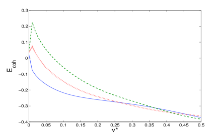
Figure 12: (Color online) Cohesive energy (in units of $e^{2}/\ell$) vs. $\nu^{*}$ for the Wigner crystal (solid line), for the 2e bubble solid (dotted line), and for the 3 electron bubble crystal (dashed line) in the $n=2$ Landau level, as obtained from the wavefunction approach of this Appendix, which is based on the symmetric gauge. The relative behavior of these cohesive energies is very similar to the behavior derived in the approach of the text based on the Landau gauge.

Appendix D Numerical values of physical quantities

In this Appendix, we give a summary of numerical values of physical quantities we use to calculate the normal modes in Sec. IV. Throughout this Appendix, we shall use CGS units, where the speed of light in vacuum $c$, Planck’s constant $h$, the electron charge $e$ and effective mass in the host semiconductor $m^{*}$ are given by

$$c = 3\times 10^{10}\;\mbox{cm/s},$$ (65a)

$$h = 6.6262\times 10^{-27}\;\mbox{erg}\cdot\mbox{s},$$ (65b)

$$e = 4.80\times 10^{-10}\;\mbox{esu},$$ (65c)

$$m^{*} = 0.067\times 9.11\times 10^{-28}\;\mbox{g}$$ (65d)

$$= 6.103\times 10^{-29}\;\mbox{g}.$$

Following Ref. Cote2003, , for the dielectric constant of the host semiconductor, we use the value $\epsilon=12.9$, relevant to GaAs, and take for the electron density the typical value $n_{0}=3.2\times 10^{11}e^{-}/cm^{2}$. The resulting expression of the magnetic field $B=n_{0}hc/e\nu$ in terms of the filling factor $\nu$ is as follows

$$B=\frac{13.24}{\nu}\times 10^{4}\mbox{Gauss}.$$ (66)

The magnetic length $\ell=\sqrt{\hbar c/eB}$ is then

$$\ell=0.7052\times 10^{-6}\sqrt{\nu}\;\mbox{cm},$$ (67)

while the effective Bohr radius $a_{B}=\hbar^{2}\epsilon/m^{*}e^{2}$ is given by

$$a_{B}=1.0188\times 10^{-6}\mbox{cm},$$ (68)

so that the ratio $a_{B}/\ell$ is given by

$$\frac{a_{B}}{\ell}=\frac{1.4426}{\sqrt{\nu}}.$$ (69)

Now, the electrostatic energy scale $e^{2}/\epsilon\ell$ is such thattypo

$$\frac{e^{2}}{\hbar\epsilon\ell}=\frac{24046.7}{\sqrt{\nu}}\;\mbox{GHz}.$$ (70)

Using Eq. (66) we obtain that the cyclotron frequency $\omega_{c}=eB/m^{*}c$ is given by

$$\omega_{c}=\frac{34741.2}{\nu}\;\mbox{GHz},$$ (71)

so that the ratio of the electrostatic to magnetic energy scales is given by

$$\frac{(e^{2}/\epsilon\ell)}{\hbar\omega_{c}}=0.692\sqrt{\nu}.$$ (72)

References

- (1) A.A. Koulakov, M.M. Fogler and B.I. Shklovskii, Phys. Rev. Lett 76, 499 (1996); M.M. Fogler, A.A. Koulakov and B.I. Shklovskii, Phys. Rev. B 54, 1853 (1996).
- (2) R. Moessner and J.T. Chalker, Phys. Rev. B 54, 5006 (1996).
- (3) R. Côté, C.B. Doiron, J. Bourassa and H.A. Fertig, Phys. Rev. B 68, 155327 (2003).
- (4) M.O. Goerbig, P. Lederer and C.M. Smith, Phys. Rev. B 69, 115327 (2004).
- (5) N. Shibata and D. Yoshioka, Phys. Rev. Lett 86, 5755 (2001); D. Yoshioka and N. Shibata, Physica A 12, 43 (2002).
- (6) F.D.M. Haldane, E.H. Rezayi and K. Yang, Phys. Rev. Lett 85, 5396 (2000).
- (7) M.P. Lilly, K.B. Cooper, J.P. Eisenstein, L.N. Pfeiffer and K.W. West, Phys. Rev. Lett. 82, 394 (1999).
- (8) R.R. Du, D.C. Tsui, H.L. Stormer, L.N. Pfeiffer, K.W. Baldwin and K.W. West, Solid State Comm. 109, 389 (1999).
- (9) Y.P. Chen, R.M. Lewis, L.W. Engel, D.C. Tsui, P.D. Ye, L.N. Pfeiffer and K.W. West, Phys. Rev. Lett. 91, 016801 (2003).
- (10) R.M. Lewis, Y.P. Chen, L.W. Engel, D.C. Tsui, P.D. Ye, L.N. Pfeiffer and K.W. West, Physica E 22, 104 (2004).
- (11) R. M. Lewis, Y. Chen, L. W. Engel, D. C. Tsui, P. D. Ye, L. N. Pfeiffer, and K. W. West, Phys. Rev. Lett. 93, 176808 (2004).
- (12) R. Chitra, T. Giamarchi and P. Le Doussal, Phys. Rev. B 65, 35312 (2001).
- (13) M.M. Fogler and D.A. Huse, Phys. Rev. B 62, 7553 (2000).
- (14) K. Maki and X. Zotos, Phys. Rev. B 28, 4349 (1983).
- (15) N.W. Ashcroft and N.D. Mermin, Solid State Physics, Saunders College Publishing, Philadelphia, 1988.
- (16) L. Bonsall and A.A. Maradudin, Phys. Rev. B 15, 1959 (1977).
- (17) S.L. Cunningham, Phys. Rev. B 10, 4988 (1974).
- (18) It should be noted that we had to perform a counterclockwise rotation of 30o of the points given by Cunningham in Ref. Cunningham1974, to align the irreducible element of the Brillouin zone implied by our lattice vectors of Eq. 22 with the one used in this last reference.
- (19) F.C. Zhang and S. Das Sarma, Phys. Rev. B 33, R2903 (1986).
- (20) I.L. Aleiner and L.I. Glazman, Phys. Rev. B 52, 11296 (1995).
- (21) P. Miranović and V.G. Kogan, Phys. Rev. Lett. 87, 137002 (2001).
- (22) D.S. Fisher, Phys. Rev. B 26, 5009 (1982).
- (23) R. Côté and A.H. MacDonald, Phys. Rev. B 44, 8759 (1991).
- (24) R. Côté, Mei-Rong Li, A. Faribault, H. A. Fertig, Phys. Rev. B 72, 115344 (2005).
- (25) Note that the value quoted in Ref. Cote2003, for , namely , is actually the numerical value of the quantity .