Dynamics in the presence of attractive patchy interactions

Abstract

We report extensive monte-carlo and event-driven molecular dynamics simulations of a liquid composed by particles interacting via hard-sphere interactions complemented by four tetrahedrally coordinated short-range attractive (”sticky”) spots, a model introduced several years ago by Kolafa and Nezbeda [J. Kolafa and I. Nezbeda, Mol. Phys. 161 87 (1987)]. To access the dynamic properties of the model we introduce and implement a new event-driven molecular dynamics algorithm suited to study the evolution of hard bodies interacting, beside the repulsive hard-core, with a short-ranged inter-patch square well potential. We evaluate the thermodynamic properties of the model in deep supercooled states, where the bond network is fully developed, providing evidence of density anomalies. We show that, differing from models of spherically symmetric interacting particles, in a wide region of packing fractions $\phi$ the liquid can be super-cooled without encountering the gas-liquid spinodal. In particular, we suggest that there is one optimal $\phi$ (not very different from the hexagonal ice $\phi$) at which the bond tetrahedral network fully develops. We find evidence of the dynamic anomalies characterizing network forming liquids. Indeed, around the optimal network packing, dynamics fasten both on increasing and decreasing $\phi$. Finally we locate the shape of the isodiffusivity lines in the $(\phi-T)$ plane and establish the shape of the dynamic arrest line in the phase diagram of the model. Results are discussed in connection to colloidal dispersions of sticky particles and gel forming proteins and their ability to form dynamically arrested states.

I Introduction

This article presents a detailed numerical study of the thermodynamics and of the dynamics of a model introduced several years ago by Kolafa and NezbedaKolafa and Nezbeda (1987) as a primitive model for water (PMW). The model envisions a water molecule as a hard sphere (HS) whose surface is decorated by four short ranged ”sticky” spots, arranged according to a tetrahedral geometry, two of which mimic the protons and two the lone-pairs. Despite its original motivation, the Kolafa and Nezbeda model is representative of the larger class of particles interacting via localized and directional interactions, a class of systems which includes, besides network forming molecular systems, also proteinsLomakin et al. (1999); Sear (1999); Kern and Frenkel (2003) and newly designed colloidal particlesManoharan et al. (2003). Indeed, recent developments in colloidal science are starting to provide particles with specific directional interactionsYethiraj and van Blaaderen (2003). In the same way as sterically stabilized colloids have become the ideal experimental model for realizing the hard-sphere fluid, novel physical chemical techniques will soon make available to the community colloidal analogs of several molecular systems. A colloidal water is probably not far from being realized.

Recent workZaccarelli et al. (2005) has focused on the dynamics of colloidal particles interacting with a restricted number of nearest neighbors. In Ref. Zaccarelli et al. (2005); Moreno et al. (2005) particles are interacting via a limited-valency square well modelSpeedy and Debenedetti (1994, 1995, 1996), imposing a many body constraint on the maximum number $n_{max}$ of bonded interactions. It has been found that when $n_{max}<6$, a significant shrinking of the liquid-gas (or colloidal rich-colloidal poor) spinodal takes place. A window of packing fractions values opens up in which it is possible to reach very low temperature (and hence states with extremely long bond lifetime) without encountering phase separation. This favors the establishment of a spanning network of long-living bonds, which in the colloidal community provides indication of gel formation but which, in the field of network forming liquids, would be rather classified as glass formation. The study of the dynamics of the PMW provides a test of the $n_{max}=4$ results, in the absence of many-body interactions and in the presence of a geometric correlation between the bonding sites, retaining the maximum valency. This article, by reporting results on a model which can be at the same time considered as a simple model for the new generation of patchy colloids or for network forming liquids, starts to bridge the gap between these two fields.

Thermodynamic and structural properties of several primitive models for water (and other bonded systems) have been studied in detail during the last 30 yearsBratko et al. (1985); Kolafa and Nezbeda (1987); Nezbeda et al. (1989); Nezbeda and Iglesias-Silva (1990); Vega and Monson (1998), since this type of primitive models have become one of the landmarks for testing theories of associationWertheim (1984a, b); Ghonasci and Chapman (1993); Sear and Jackson (1996); Duda et al. (1998); Peery and Evans (2003); Kalyuzhnyi and Cummings (2003). In particular, the theory of WertheimWertheim (1984a, b) has been carefully compared to early numerical studies, suggesting a good agreement between theoretical predictions and numerical data, in the temperature and packing fraction regions where it was possible to achieve numerical equilibrationVega and Monson (1998). Recently, the increased numerical facilities, extending the range of studied state points, have clarified that deviations from the theoretical predictions start to take place as soon as the number of bonds (between different patches) per molecule increases and a network of bonded particles appearsVlcek et al. (2003); Duda et al. (1998). Geometric correlations between different bonds, not included in the theory, are responsible for the break down of the theoretical and numerical agreement. Attempts to extend the perturbation theory beyond first order do not appear to be able to cure the problemVlcek et al. (2003). The PMW is a good candidate for testing new theories of association and, for this reason, it is important to clearly establish numerically the low $T$ behavior of the supercooled liquid state. The equilibrium PMW phase diagram, recently calculatedVega and Monson (1998), includes two crystal regions and a metastable fluid-gas coexistence.

All previous studies of primitive models for sticky directional interactions have focused on thermodynamic and static properties of the model. But the ability of fully exploiting the fast developments taking place in colloidal physics Glotzer (2004); Zhang and Glotzer (2004) requires understanding not only the equilibrium phases of systems of patchy particles and their modifications with the external fields, but also understanding the kinetic phase diagramSciortino (2002), i.e. the regions in phase space where disordered arrested states can be expected, and when and how these states are kinetically stabilized with respect to the ordered lowest free energy phases. In this respect, it is worth starting to establish the dynamic properties of simple models of patchy interactions, since the simplicity of these models (based on hard sphere and square well interactions) have the potentiality to provide us with an important reference frame and may play a relevant role in deepening our understanding of the dynamic arrest in network forming liquids, in connecting arrest phenomena associated to gel formationZaccarelli et al. (2005); Gado and Kob (2005) (the establishment of a percolating network of long lived bonds) and arrest related to excluded volume effects and the dependence of the general dynamic and thermodynamic features on the number and spatial location of patchy interactions. The case of the PMW reported here is a good starting one. In this article we report thermodynamic data, extending the previously available information to lower temperatures and, for the first time, dynamic information obtained solving the Newton equations using a new algorithm based on event-driven propagation.

II The Model and Numerical Details

In the PMW, each particles is composed of an hard sphere of diameter $\sigma$ (defining the length scale) and by four additional sites located along the direction of a tetrahedral geometry. Two of the sites (the proton sites H) are located on the surface of the hard sphere, i.e. at distance $0.5\sigma$ from the center. The two remaining sites (the lone-pair sites LP) are located at distance $0.45\sigma$. Besides the hard-sphere interaction, preventing different particles to sample distances smaller than $\sigma$, only the H and LP sites of distinct particles interact via a square well (SW) potential $u_{SW}$ of width $\delta=0.15\sigma$ and depth $u_{0}$, i.e.

$$u_{SW}=-u_{0}~{}~{}r<\delta$$ (1)

$$~{}~{}~{}~{}~{}=0~{}~{}~{}~{}~{}~{}r>\delta,$$

where $r$ is here the distance between H and LP sites. The choice of $\delta=0.15\sigma$ guarantees that multiple bonding can not take place at the same site. The depth of the square well potential $u_{0}$ defines the energy scale. Bonding between different particles is thus possible only for specific orientations and distances. In the linear geometry, the maximum center-to-center distance at which bonding is possible is $1.1\sigma$ since the LP site is buried $0.05\sigma$ within the hard-core, a value typical of short-range colloid-colloid interactions.

We have studied a system of $N=350$ particles with periodic boundary conditions in a wide range of packing fraction $\phi\equiv\pi/6n\sigma^{3}$ (where $n$ is the number density) and temperatures $T$, where $T$ is measured in units of $u_{0}$ ($k_{B}=1$). We perform both Monte Carlo (MC) and event driven molecular dynamics. In one MC step, an attempt to move each particle is performed. A move is defined as a displacement in each direction of a random quantity distributed uniformly between $\pm 0.05~{}\sigma$ and a rotation around a random axis of random angle distributed uniformly between $\pm 0.5$ radiant. Equilibration was performed with MC, and monitored via the evolution of the potential energy (a direct measure of the number of bonds in the system). The mean square displacement (MSD) was also calculated to guarantee that each particle has diffused in average more than its diameter. In evaluating the MSD we have taken care of subtracting the center of mass displacement, an important correction in the low $T$ long MC calculations. At low $T$ simulations required more than $10^{9}$ MC steps, corresponding to several months of CPU time.

We have also performed event driven (ED) molecular dynamic simulations of the same system, modeling particles as constant density spheres of diameter $\sigma$ and mass $m$. The momentum of inertia is diagonal and equal to $m\sigma^{2}/10$ . The algorithm implemented to propagate the newtonian trajectory in the presence of patchy square well interaction is described in details in Appendix VII. In ED dynamics, time is measured in units of $\sigma\sqrt{m/u_{0}}$. Assuming as $m$ the mass of the water molecule, as $u_{0}$ a typical value for hydrogen bond ($\approx 20kJ/mol)$ and as $\sigma$ the nearest neighbor distance in water ($0.28nm$), the unit of time corresponds $\approx 0.3ps$. All static quantities have been evaluated with both MC and MD configurations finding no differences.

Pressure, measured in units of $u_{0}/\sigma^{3}$, has been calculate as sum of three contributions. A trivial kinetic contribution, equal to $nk_{B}T$. A positive HS contribution and a negative contribution arising from the SW interaction. Details of the calculation of $P$ in both MC and ED simulations is provided in the Appendix VIII.

III Results: Static

III.1 Potential Energy $E$

Since in the PMW each site can take part to only one bond, due to geometric constraints fixed by the small value of $\delta$, the lowest energy configuration is defined by four bonds per particles, corresponding to a ground state energy per particle $E_{gs}=-2$ (in units of $u_{0}$). Of course, this absolute ground state value may not be accessible at all $\phi$, due to the strong constraints introduced by the bonding geometry. According to Wertheim’s first order thermodynamic perturbation theory, the $T$ and $\phi$ dependence of the potential energy per particle $E$ is given byKolafa and Nezbeda (1987); Nezbeda et al. (1989); Vega and Monson (1998)

$$E-E_{gs}=\frac{2}{1+c}$$ (2)

where

$$c=0.5\bigg{\{}\left[1+192(e^{\frac{1}{T}}-1)\phi J\right]^{0.5}-1\bigg{\}}$$ (3)

$$J=\frac{c_{1}(1-\phi/2)-c_{2}\phi(1+\phi)}{(1-\phi)^{3}}$$ (4)

with $c_{1}=2.375\times 10^{-5}$ and $c_{2}=2.820^{-6}$Vega and Monson (1998). The Wertheim theory, which assumes uncorrelated independent bonds, predicts as low $T$ limit of Eq. 2 an Arrhenius $T$-dependence,

$$\lim_{T\rightarrow 0}E-E_{gs}=\frac{4}{\sqrt{192\phi J}}e^{-0.5/T}$$ (5)

i.e. with an activation energy of half bond energy. It is worth observing that such an Arrhenius law, with an activation energy equal to $0.5$ characterizes the low $T$ dependence of the energy in the $n_{max}$ modelMoreno et al. (2005); Zaccarelli et al. (2005) [a model of particles interacting via a SW potential with an additional constraint on the maximum number of bonds], where no geometric correlation between bonds is imposed.

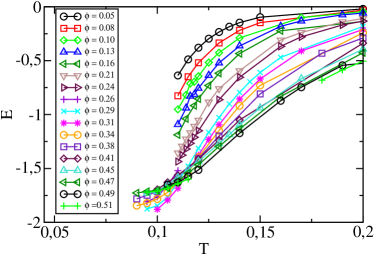
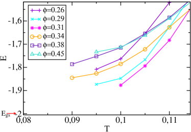
Figure 1: Potential energy for the PMW. The top panel shows data for all studied isochores as a function of $T$. The lower panel shows an enlargement of the low $T$ region, where the network is fully developed. Note that for this model, the lowest possible energy is $E_{gs}=-2$.

Fig. 1 shows the $T$ dependence of the potential energy for different isochores. As discussed in details in the following, for $\phi\lesssim 0.24$ a phase separation is encountered on cooling, preventing the possibility of equilibrating one-phase states below $T\approx 0.11$. For $\phi>0.24$ the system remains homogeneous down to the lowest investigated $T$. The low $T$-behavior is expanded in Fig. 1-(bottom). With the extremely long equilibration runs performed, proper equilibration is reached only for $T\gtrsim 0.09$. The enlargement of the low $T$ region shows that the absolute ground state value $-2u_{0}$ is closely approached at $\phi\approx 0.3$. At higher or smaller $\phi$, the potential energy appear to approach a constant value larger than $-2u_{0}$. Consistent with previous claimsVega and Monson (1998), high $T$ data are very well represented by first order thermodynamic perturbation theory. Systematic deviations between theory and simulation data appears as soon as the number of bonds per particle becomes bigger than one. Comparing the simulation data with the Wertheim theory, it is confirmed that the physics of the network formation is completely missing in the first-order perturbation theory.

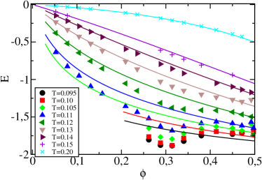
Figure 2: Potential energy vs. $\phi$ along isotherms. Symbols: simulation data. Lines: Wertheim’s theory.

Fig. 2 shows the $\rho$ dependence of $E$ along isochores. At high $T$ ($T>0.13$), a monotonic decrease of $E$ is observed, caused by the increased bonding probability induced by packing. In this $T$ region, the number of bonds is at most of the order of two per particle. Completely different is the situation for lower $T$. The $\phi$ dependence becomes non-monotonic. There is a specific value of the packing fraction ($\phi\approx 0.3$) at which the lowest energy states are sampled. In the following we define the optimal network packing fractions as the range of packing fractions for which it is possible to fully satisfy the bonds in a disordered homogeneous structure. At $\phi\approx 0.3$, the number of bonds at the lowest investigated $T$ (the lowest $T$ at which equilibration is feasible with several months of computation time) is about $3.8$ per particle, i.e. about 95% of the bonds are satisfied. The range of optimal $\phi$s appears to be rather small. Indeed for packing fractions lower or higher than this optimal $\phi\approx 0.314$, the formation of a fully connected network is hampered by geometric constraints: at lower $\phi$, the large inter-particle distance acts against the possibility of forming a fully connected network, while at large $\phi$, packing constraints, promoting close packing configurations are inconsistent with the tetrahedral bonding geometry. Not surprisingly, $\phi=0.314$ is within the range of $\phi$ values which allow for a stable open diamond crystal phase ($0.255<\phi<0.34$)Vega and Monson (1998). A reduction of the geometric constraints (as in the $n_{max}$ modelZaccarelli et al. (2005, 2005)) increases the range of optimal $\phi$. It is worth also noting that the liquid side of the spinodal curve is close to the region of optimal network $\phi$.

The existence of a convex form for the potential energy (here for $\phi\gtrsim 0.3$) has been observed in several other models for tetrahedral networks, including models for water (and water itselfSciortino et al. (1997a)). It has been pointed out that a negatively convex $\phi$ dependence is indicative of a destabilization of the free energySciortino et al. (1997a) and a precursor of a possible liquid-liquid critical point (in addition to the lower $\phi$ gas-liquid one). Liquid-liquid critical points have been observed in several models for waterPoole et al. (1992, 1993); Yamada et al. (2002); Poole et al. (2005); Paschek (2005); Brovchenko et al. (2005). Indeed, the Helmholtz free energy $A$ is related to $U$ (the sum of the kinetic and potential energy) via $A=U-TS$, where $S$ is the entropy. The curvature of an isotherm of $A$ must be positive for a homogeneous phase of a specified volume $V$ to be thermodynamically stable. The curvature of $A$ can be expressed as

$$\left(\frac{\partial^{2}A}{\partial V^{2}}\right)_{T}=\left(\frac{\partial^{2}U}{\partial V^{2}}\right)_{T}-T\left(\frac{\partial^{2}S}{\partial V^{2}}\right)_{T}$$ (6)

Since $P=-\left(\frac{\partial A}{\partial V}\right)_{T}$ the inverse compressibility $K_{T}=-1/V(\partial V/\partial P)_{T}$ is related to the curvature of $A$ by

$$\frac{1}{K_{T}}=V\left[\left(\left(\frac{\partial^{2}U}{\partial V^{2}}\right)_{T}-T\left(\frac{\partial^{2}S}{\partial V^{2}}\right)_{T}\right)\right]$$ (7)

The curvature of $A$ is thus proportional to $1/K_{T}$ for fixed $V$. Since $1/K_{T}$ must be positive for a thermodynamically stable state, for the range of $V$ in which $\left(\frac{\partial^{2}U}{\partial V^{2}}\right)_{T}<0$, the contribution of the internal energy reduces the thermodynamic stability of the liquid phase. The liquid remains stable where $U$ has negative curvature only because the contribution of the entropic term in Eq.  6 is large enough to dominate. Yet entropic contributions to these thermodynamic quantities are suppressed as $T$ decreases, due to the occurrence of the factor of $T$ in the second term on the right-hand side of Eq. 6. Hence the $U-V$ data suggest that at lower $T$ a single homogeneous phase of the liquid will not be stable for certain values of $V$, leading to a separation into two distinct liquid phases of higher and lower volume. Due to the predominant role of $E$ in the free energy at low $T$, the possibility of a phase separation of the PMW liquid into two liquid phases of different $\phi$, for $\phi>0.3$ and $T$ lower than the one we are currently able to equilibrate should be considered.

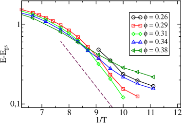
Figure 3: Arrhenius representation ($E-E_{gs}$ vs $1/T$) of the potential energy around the optimal network density. The dashed line, shown as a reference, has an activation energy of $-u_{0}$.

Fig. 3 shows $\ln(E-E_{gs})$ vs $1/T$. At the optimal $\phi$, the energy of the fully connected state is approached with an Arrhenius law, characterized by an activation energy of $\approx 1u_{0}$, clearly different from the $0.5$ value predicted by the Wertheim theory. For larger $\phi$ values, data suggest that the lowest reachable state has an energy different from $-2u_{0}$, consistent with the expectation that on increasing $\phi$, geometric constraints forbid the development of a fully connected network even at the lowest $T$.

III.2 $P$

The Wertheim’s prediction for the $T$ and $\phi$ dependence of the PMW pressure (the equation of state) is

$$P=P_{HS}~{}~{}~{}~{}~{}$$ (8)

$$-nk_{B}T\frac{96(e^{1/T}-1)}{(1+c)^{2}}\frac{c_{1}\phi(1+\phi-0.5\phi^{2})-2c_{2}\phi^{2}(1+2\phi)}{(1-\phi)^{4}}$$

where $P_{HS}$ is the pressure of the HS fluid at the same packing fraction. $P_{HS}$ is very well represented by the Carnahan-Starling EOSHansen and McDonald (1986)

$$P_{HS}=nk_{B}T\frac{(1+\phi+\phi^{2}-\phi^{3})}{(1-\phi)^{3}}$$ (9)

The Wertheim EOS predicts a vapor-liquid critical point at $T_{c}=0.1031$ and $\phi_{c}=0.085$Vega and Monson (1998). The vapor-liquid spinodals calculated according to the Wertheim theory and from simulation data are reported in Fig. 4. The numerical estimate is provided by locating, along isochores, the highest $T$ state point in which phase separation is observed and the $T$ at which the small $q$ limit of the structure factor is smaller than five. These two state points bracket the spinodal locus. It is interesting to compare the liquid-gas spinodal of the PMW with the corresponding spinodal of the symmetric spherical square well potential with same depth and well width $\delta=0.15$. In that case, the critical point is located at $T_{c}\approx 0.56$ and $\phi_{c}\approx 0.212$Pagan and Gunton (2005) and the high packing fraction (the liquid) side of the spinodal extends beyond $\phi=0.6$. The net result of decreasing the surface available to bonding and of limiting to four the maximum number of nearest neighbors which can form bonds is the opening of a wide region of $\phi$ values where (in the absence of crystallization) an homogeneous fluid phase is stable (or metastable). This finding is in full agreement with the recent work of Zaccarelli et al. (2005), where a saturated square well model was studied for different values of the maximum valency. Indeed, it was found that when the number of bonds becomes less then six, the unstable region (the surface in the $(\phi-T)$ plane encompassed by the spinodal line) significantly shrinks, making it possible to access low $T$ states under single phase conditions.

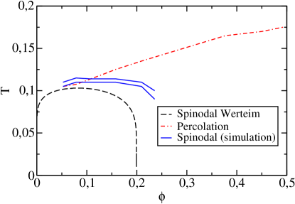
Figure 4: Thermodynamic phase diagram for the PMW. The theoretical Wertheim prediction for the locus at which $(\partial P/\partial V)_{T}=0$ is compared with numerical estimates of the spinodal, calculated by bracketing it via the locus of point at which $S(0)\approx 5$ and the locus of points where a clear phase separation is detected. The location of the bond percolation line is also reported.

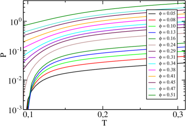
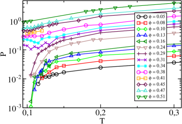
Figure 5: Isochores of $P$ according to the Wertheim theory (top) and as calculated from the simulation data (bottom). Symbols refer to simulation data. The same sequence of $\phi$ values is shown in both panels.

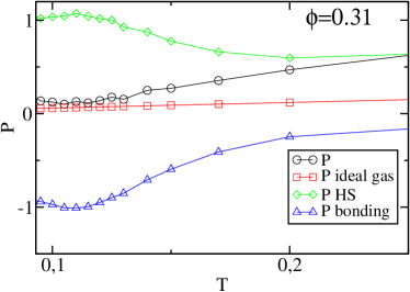
Figure 6: Components of the pressure at $\phi=0.314$. The total $P$ is decomposed in ideal gas, HS and bonding components. Note the isochoric minimum in $P$ around $T=0.105$, a signature of an isobaric density maximum.

Fig. 5 shows $P(T)$ for different isochores. In agreement with previous analysis, $P$ is well represented by the Wertheim theory only at high temperature. At low $T$ several interesting features are observed: (i) for $\phi<0.25$, isochores end in the spinodal line. (ii) in the simulation data, a clear difference in the low $T$ behavior is observed between the two studied isochores $\phi=0.288$ and $\phi=0.314$ . While in the $\phi=0.288$ case $P(T)$ decreases continuously on cooling, in the $\phi=0.314$ case the low $T$ behavior of $P$ is reverses and $P$ approaches a positive finite value on cooling. This different low-$T$ trends indicated that for $\phi\lesssim 0.3$, on cooling the network becomes stretched (negative pressures), in the attempt to preserve the connected bonded state. This implies that at low $T$, there is a driving force for phase separating into a fully connected unstressed network and a gas phase. This also suggests that the spinodal curve ends at $T=0$ around $\phi=0.3$. At $\phi\approx 0.3$, the packing fraction is optimal for the formation of an unstressed fully connected network at low $T$. The bond formation on cooling does not require any stretching and it reverses the $T$-dependence of $P$. (iii) Between $0.3\lesssim\phi\lesssim 0.38$ a minimum of $P$ appears. The existence of a minimum in $P(T)$ along isochores evidences the presence of density anomalies (i.e. expansion on cooling along isobars) since points in which $(\partial P/\partial T)_{V}=0$, by a Maxwell relation, coincide with points in which $\alpha\equiv(\partial V/\partial T)_{P}=0$, i.e. with points in which density anomalies are present. The simplicity of the model allows us to access the different contributions to $P$ and investigate the origin of the increase of $P$ on cooling. In the PMW, apart from the trivial kinetic component contribution, the only positive component to $P$ arises from the HS interaction. Interestingly enough, the HS component increases on cooling. Such an increase in the HS repulsion, indirectly induced by the formation of the bonding pattern, in the range $0.30\lesssim\phi\lesssim 0.36$ appears to be able to compensate the decrease in the bonding component of $P$.

To confirm the presence of density anomalies it is instructive to look at the $V$ dependence of $P$ along isotherms, shown in Fig. 7. Again, the simulation data are consistent with the Wertheim theory predictions only at large $T$ and indeed it was already noted that no density anomalies are found within the theoryKolafa and Nezbeda (1987). The simulation data also show a clear crossing of the isotherms around a volume per particle $v=1.4$ and $1.7$, corresponding to $\phi=0.314$ and $\phi=0.38$. Again crossing is indicative of the presence of density anomalies. The increase of $P$ on cooling, between $\phi=0.314$ and $\phi=0.38$ suggest also a possible emergence of a second Van der Waal-type loop (in addition to the gas-liquid one) for $T$ lower than the one we are currently able to equilibrate. The possibility of a second critical point between two liquid phases of different densities has been discussed at length in the pastSciortino (2005), following the discovery of itPoole et al. (1992) in one of the first models for waterStillinger and Rahman (1974).

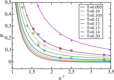
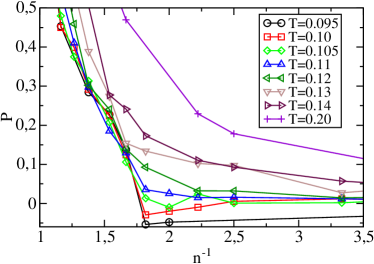
Figure 7: Isotherms of $P$ according to the Wertheim theory (top) and as calculated from the simulation data (bottom) as a function of the volume per particle $v\equiv n^{-1}$. Symbols refer to simulation data. Note the crossing of the different isotherms at $v=1.4$ and $1.7$.

III.3 $g(r)$

The PMW radial distribution functions for $T>0.15$, have been reported previouslyKolafa and Nezbeda (1987). Here we focus on the interesting structural changes observed during the development of the bond network in $g_{OO}$ and $g_{H-LP}$, a $T$-region which was not possible to access in the previous simulations. The $g_{OO}$ provides information on the center to center particle correlation while $g_{H-LP}(r)$ contains information on the bonding and on the attractive component of the pressure.

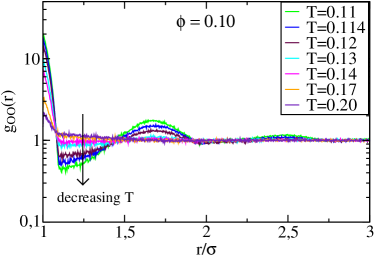
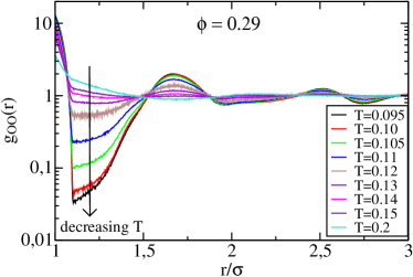
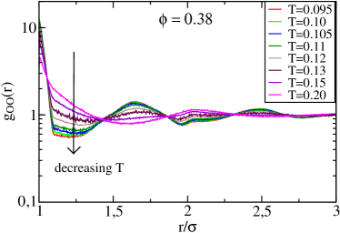
Figure 8: Particle-particle radial distribution function at $\phi=0.105$, $\phi=0.288$, $\phi=0.380$.

Fig. 8 shows $g_{OO}(r)$ at three different packing fractions. In the interval $1<r<1.1$ the function is highly peaked, a consequence of the distance imposed by bonding. Outside the bonding distance ($r>1.1$), $g_{OO}(r)$ shows significant oscillations only at low $T$. A peak, beside the bonding one, is observed at $r\approx 1.7$ corresponding to the characteristic distance between two particles bounded to the same central particle in a tetrahedral geometry. The absence of the information about the geometry of the bonding sites in the theory of Wertheim is responsible for the absence of the peak at $1.7\sigma$ and the breakdown of the predictive ability of the Wertheim theory as soon as a particle is engaged in more than two bonds. A few observations are in order when comparing the $\phi$ dependence of $g_{OO}(r)$: At low $\phi$, the tetrahedral peak at $r\approx 1.7$ is the only peak in $g_{OO}(r)$. When $\phi$ approaches the optimal network density a clear tetrahedral pattern develops and $g_{OO}(r=1.7)$ becomes larger than two. The tetrahedral peaks at $\approx 1.7$ is followed by oscillations extending up to $4\sigma$. At even larger $\phi$, there is still a residual signature of tetrahedral bonding at $1.7\sigma$, but the depletion region for $r>1.1\sigma$ is not developed any longer, signaling a competition between the HS packing (which favor a peaks at positions multiple of $\sigma$) and the local low density required by bonding.

Fig. 9 compares, at $\phi=0.314$, the OO, HH and H-LP radial distribution functions in linear scale. In all three functions, the progressive structuring induced by the bonding is clearly evident. Even $g_{HH}(r)$ shows very clear signs of spatial correlations, which are induced by the tetrahedral geometry of the bonding and by the geometry by which the bonding between $H$ and $LP$ propagates. Indeed, in the PMW model the interaction between different $H$ sites is zero.

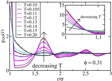
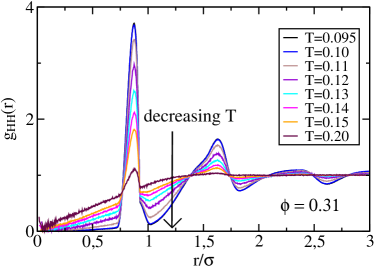
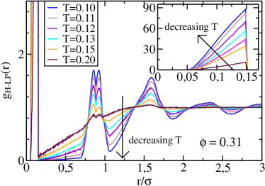
Figure 9: Radial distribution functions for $OO$, $HH$ and $H-LP$ pairs at the optimal network density $\phi=0.314$. Insets in $g_{OO}$ and $g_{{}_{H-LP}}$ provide enlargements of the contact region. On cooling a significant structure appears, associated to the intense bonding.

III.4 $S(q)$

The structure factor of the system, defined in term of the particle’s center coordinates $\vec{r}_{i}$ as,

$$S(\vec{q})=<\frac{1}{N}\sum_{i=1}^{N}e^{i\vec{q}\cdot(\vec{r}_{i}-\vec{r}_{j})}>$$ (10)

provides information on the wave vector dependence of the density fluctuations. In isotropic systems, $S(q)$ is function of the modulus $q$. The behavior of $S(q)$ at small $q$ provides indication on the phase behavior, since an increase of $S(q)$ at small $q$ indicates the development of inhomogeneities with length-scale comparable to the system size studied. As an indicator of the location of the phase boundaries (of the liquid-gas spinodal line), we estimate the locus of points in $(T,\phi)$ where $S(q)$ for the particles centers becomes larger than 5 at small $q$. This locus is reported in Fig. 4. For $\phi\gtrsim 0.28$ $S(q)$ does not show any sign of growth at small $q$ in the region of $T$ where equilibration is feasible, being characterized by values of $S(q)$ at small $q$ of the order of $0.1$. This confirms that, at this packing fraction, there is no driving force for phase separation, since the average density has reached a value such that the formation of a fully connected network of bonds does not require a local increase of the packing fraction. It is also important to stress that at $\phi=0.288$, at the lowest studied $T$, the average number of bond per particle is $3.8$, and hence the system is rather close to its ground state and no more significant structural changes are expected on further cooling.

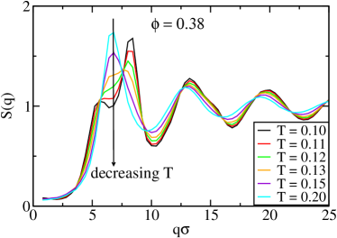
Figure 10: Particle-particle structure factor at $\phi=0.105$, $\phi=0.288$, $\phi=0.3858$. Note that at $\phi=0.105$, an intense signal develops at small $q$, related to the approach to the spinodal instability. Small $q$ intensity is completely missing at the higher $\phi$ shown.

Fig. 10 shows $S(q)$ at $\phi=0.105$, $\phi=0.288$ and $\phi=0.385$. The $\phi=0.105$ case has been chosen to show the significant increase in $S(q)$ associated to the approach of the spinodal curve. The case $\phi=0.288$ shows both the absence of a small $q$-vector divergence and the clear development of the typical $q$-pattern of tetrahedral networks. On cooling the peak at $q\sigma=2\pi$, characteristic of excluded volume interactions splits in two parts. A pre-peak around $q\sigma\approx 5$ and an intense peak around $q\sigma\approx 8$. The case $\phi=0.385$ confirms that the packing fraction is now so high that a full tetrahedral network cannot develop and the splitting of the main peak in two distinct components is very weak and visible only at the slowest investigated $T$.

III.5 Percolation

The PMW, as all other models based on HS and SW interactions, is particularly suited for calculation of bond properties, since a bond between particle $i$ and $j$ can be unambiguously defined when the pair interaction energy between $i$ and $j$ is $-u_{0}$. In the case of continuous potentials such a clear cut bond definition is not possible and several alternative propositions have been put forwardHill (1987); Coniglio et al. (2004). We focus here on the connectivity properties of the equilibrium configurations. We use standard algorithms to partition particles into clusters. Configurations are considered percolating when, accounting for periodic boundary conditions, an infinite cluster is present. More explicitly, to test for percolation, the simulation box is duplicated in all directions and the ability of the largest cluster to span the replicated system is controlled. If the cluster in the simulation box does not connect with its copy in the duplicated system then the configuration is assumed to be non-percolating. The boundary between a percolating and a non-percolating state point has been defined by the probability of observing infinite clusters in 50$\%$ of the configurations. The resulting percolation line is reported in Fig. 4. State points on the right side of the line are characterized by the presence of an infinite cluster. Still, at this level of definition, percolation is a geometric measure and it does not provide any information on the lifetime of the percolating cluster.

The percolation line, like in simple SW potentials, crosses the spinodal curve very close to the critical point. Differently from the SW, the percolation locus does not extend to infinite $T$, since at high $T$, even at large $\phi$, the reduce particle surface available for bonding prevents the possibility of forming a spanning network with a random distribution of particles orientations. Along the percolation line, about 1.5 bonds per particle are observed, with a small trend towards an increase of this number on decreasing $\phi$. In terms of bond probability $p_{b}$, this correspond to $p_{b}\approx 0.375$, not too different from the bond percolation value of the diamond lattice, known to be $0.388$Stauffer and Aharony (1992).

IV Dynamics

Thermodynamic and static properties of the PMW presented in the previous section clarify the location of the regions in which the bond network forms, the region where the liquid-gas phase separation takes place and the region at high $\phi$ where packing phenomena start to be dominant. In the following we present a study of the diffusion properties of the model in the phase diagram, with the aim of locating the limit of stability of the liquid state imposed by kinetic (as opposed to thermodynamic) constraints.

IV.1 $MSD$

We focus on the mean square displacement $<r^{2}(t)>$ of the particle centers, as a function of $T$ and $\phi$, calculated from the newtonian dynamic trajectories. Fig. 11 shows $<r^{2}(t)>$ for a few selected isochores. For short time $<r^{2}(t)>=<v_{T}^{2}>t^{2}$, where $<v_{T}^{2}>=3/2k_{B}T$ is the thermal velocity. At high $T$, the short-time ballistic behavior crosses over to a diffusion process ($<r^{2}>\sim t$) directly. At low $T$, the ballistic short-time and the diffusive long time laws are separated by an intermediate time window in which $<r^{2}(t)>$ is approximatively constant, an indication of particle caging.

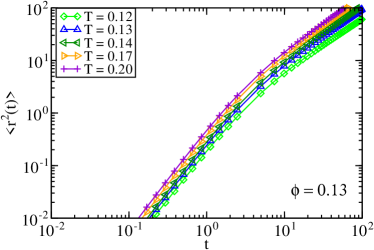
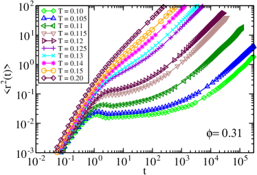
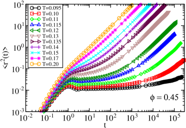
Figure 11: Mean square displacement for different $T$s, at three different $\phi$ values. Top: $\phi=0.131$, Center: $\phi=0.314$, Bottom: $\phi=0.450$.

Several features of $<r^{2}(t)>$ are worth pointing: (i) For $\phi\lesssim 0.209$, the spinodals are encountered on cooling before the caging process is visible. The phase separation process sets in well before particles start to feel the caging process. (ii) The static percolation curve reported in Fig. 4 has no effect on dynamics. There is no dynamic arrest at the static percolation transition. (iii) For $\phi$ such that a well developed tetrahedral network can form, it is possible to cool the system down to temperatures at which, on the scale of simulation, arrest is observed, in the absence of any phase separation. $<r^{2}(t)>$ develops a clear intermediate region where only the dynamic inside the cage is left. At this $\phi$, the caging is not associated to excluded volume interactions, but to the formation of energetic bondsSciortino et al. (1996). (iv) The plateau value in $<r^{2}(t)>$ is a measure of the localization length induced by the cage. To visualize the $\phi$ dependence of the localization length, we show in Fig. 12 $<r^{2}(t)>$ for three different state points ($\phi$-$T$) with the same long time diffusivity. The cage length is always significantly larger than the typical $HS$ value ($<r^{2}(t)>\sim 0.01)$ and grows on decreasing $\phi$.

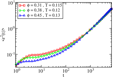
Figure 12: Mean square displacement along a constant $D$ path. Note the $\phi$ dependence of the plateau at intermediate times, which provides an estimate of the caging length.

IV.2 Diffusion Coefficient

The long time limit of $<r^{2}(t)>$ is, by definition, $6Dt$, where $D$ is the diffusion coefficient. The $\phi$ and $T$ dependence of $D$ is shown in Fig. 13. We show $\log(D)$ both vs. $T$ and vs $1/T$. Again, a few considerations are in order: (i) The range of $D$ data covers about five orders of magnitude. The data for $\phi<0.24$ are limited in $T$ by the phase separation process, while the data for $\phi>0.26$ are limited by computational resources, since equilibration can not be reached within several months of calculations. (ii) Data for $\phi>0.26$ crosses around $T\approx 0.105$, suggesting a non monotonic behavior of the $\phi$ dependence of the dynamics. (ii) The early decay of $D$ with $T$ can be described with a power-law $|T-T_{MCT}|^{\gamma}$. Power law fits, limited to the region of $T$ between $T=0.11$ and $T=0.15$, cover the first two-three orders of magnitude in $D$, in agreement with previous studies of more detailed models for waterGallo et al. (1996); Sciortino et al. (1996); Starr et al. (1999a) and with the previously proposed MCT interpretation of themGallo et al. (1996); Fabbian et al. (1999a); Sciortino et al. (1997b); Fabbian et al. (1998). (iii) A cross-over to an Arrhenius activated dynamics is observed at low $T$. Activated processes become dominant in controlling the slowing down of the dynamics. The activation energy is $\approx 4$ close to the optimal network $\phi$, suggesting that at low $T$ diffusion requires breaking of four bonds. The cross-over from an apparent power-law dependence to an Arrhenius dependence has also been observed in simulations of other network forming liquids, including silicaHorbach and Kob (1999); Saika-Voivod et al. (2001) and more recently waterXu et al. (2005). The low $T$ Arrhenius dependence also suggests that in the region where bonding is responsible for caging the vanishing $D$ locus coincides with the $T=0$ line.

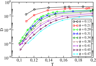
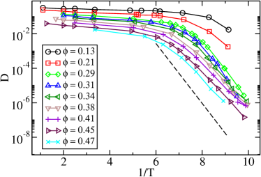
Figure 13: Temperature dependence of the diffusion coefficient along isochores. The dashed line is an Arrhenius dependence with activation energy equal to $4$.

Particularly interesting is the behavior of $D(\phi)$ along isotherms. An almost linear dependence at small $\phi$ (up to $\phi=0.235$) is followed by a non monotonic behavior. Below $T=0.11$, a diffusion anomaly is observed in the $T$ and $\phi$ region where the tetrahedral network develops. Around $\phi=0.34$ an isothermal compression of the system generates a speed up of the dynamics. Above $\phi\approx 0.35$, $D$ starts to decrease again on increasing packing. Diffusivity anomalies of the type observed in the PMW are found in several tetrahedral network forming liquids, including waterScala et al. (2000). The explanation for this counterintuitive $\phi$ dependence of the dynamics is to be found in the geometric constraints requested by the tetrahedral bonding requiring an open local structure. Increasing $\phi$ destroys the local bonding order with a resulting speed up of the dynamics.

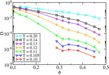
Figure 14: Diffusion coefficient along isotherms. Note the non-monotonic behavior which develops for $T<0.11$.

IV.3 Isodiffusivity (and arrest) lines

A global view of the dynamics in the $(T-\phi)$ plane is offered by the isochronic lines, i.e. the locus of state points with the same characteristic timeTölle (2001). In the present case we focus on the isodiffusivity lines. The shape of the isodiffusivity lines, extrapolated to $D\rightarrow 0$ provides a useful indication of the shape of the glass transition lineFoffi et al. (2002); Zaccarelli et al. (2002); Sciortino et al. (2004). Fig. 15 shows the isodiffusivity lines for several different values of $D$, separated each other by one order of magnitude. The slowest isodiffusivity lines are only weakly $T$ dependent at low $\phi$. For small values of $D$, iso-diffusivity lines start from the right side of the spinodal, confirming that slow dynamics is only possible for states with $\phi>\phi_{c}$. At large $\phi$ the isodiffusivity lines bend and become parallel to the $T$ axis, signaling the cross-over to the hard-sphere case. Extrapolating to zero the $T$ (or $\phi$) -dependence of $D$ it is possible to provide estimates of the dynamic arrest line. In the present model, the low $T$-dependence of $D$ along isochores is well modeled by the Arrhenius law and hence technically arrest is expected at $T=0$. The shape of the iso-diffusivity lines suggests that the vertical repulsive glass line (controlled by excluded volume effects) starting at high $T$ from the HS glass packing fraction meets at a well defined $\phi$ the $T=0$ bond glass line.

The shape of the PMW isodiffusivity lines is very similar to the short-range square well case, for which a flat $T$-independent ”attractive” glass line crosses (discontinuously) into a perpendicular $\phi$ independent ”repulsive” glass lineDawson et al. (2001); Zaccarelli et al. (2002). Differently from the SW case, in the PMW the equivalent of the attractive glass line extends to much smaller $\phi$ values, since the reduced valency has effectively reduced the space in which phase separation is observedZaccarelli et al. (2005). It is also worth pointing that the shape of the isodiffusivity lines at low $\phi$ is similar to the shape of the percolation line. As in all previously studied modelsZaccarelli et al. (2002, 2005), crossing the percolation line does not coincide with dynamics arrest, since the bond lifetime is sufficiently short that each particle is able to break and reform its bonds.

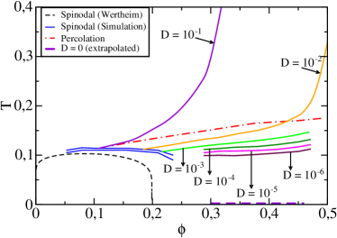
Figure 15: Isodiffusivity lines in the $(T-\phi)$ plane. An excursion of five orders of magnitude in $D$ values is explored. All lines start from the spinodal and end at infinite $T$ at the corresponding HS location. At small $D$, lines cannot be continued above $\phi=0.5$ since there the HS interaction is dominant and the system crystallizes. Extrapolating along isochores the observed Arrhenius functional form suggest an ideal $D=0$ arrest line at $T=0$.

IV.4 $D$ vs. $E-E_{gs}$

At the optimal network density, the low $T$ behavior of both $D$ and $E-E_{gs}$ (which, as discussed above, is also a measure of the number of broken bonds) is Arrhenius. This suggests to look more carefully in the relation between the activation energy of the two processes. One possibility is offered by a parametric plot of $D$ vs $E-E_{gs}$ in log-log scale, so that the slope of the straight line provides the ratio of the two activation energies. Such a plot is shown in Fig. 16. We find the remarkable results that close to the optimal network $\phi$, the slope of the curve has exponent four, i.e. $D\sim(1-p_{b})^{4}$, where $p_{b}$ is the probability that one of the four bonds is formed (and hence $1-p_{b}$ is the probability that one of the four possible bonds is broken), suggesting that the elementary diffusive process requires the breaking of four bonds. A functional law for diffusion in a tetrahedral model of this type was proposed by TeixeraTeixeira (1990) to interpret the $T$ dependence of $D$ in water in the context of the percolation model developed in Ref. Stanley and Teixeira (1980). A similar dependence has been recently reported for a model of gel-forming four-armed DNA dendrimersStarr and Sciortino (2005).

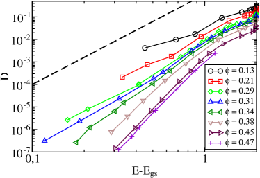
Figure 16: Diffusion Coefficient vs $E-E_{gs}$ for different $\phi$ values. The dashed line is a power-law with exponent four.

IV.5 $D$ - MD vs. MC

All dynamic data presented above refer to event-driven newtonian dynamics. Indeed, Monte Carlo simulations intrinsically miss dynamic informations being based, in their simpler formulations, on random displacements of the individual particles. Still, if the random displacement in the trial move is small as compared to the particle size the sequence of MC steps can be considered a possible trajectory in configuration space. When this is the case, the number of MC-steps (each step being defined as an attempted move per each particle) plays the role of time in the evolution of the configurations in configuration space. In the absence of interactions, a particle evolved according to the MC scheme diffuses with a bare diffusion coefficient $D_{MC}^{0}$ fixed by the variance $\delta_{MC}^{2}$ of the chosen random displacement along each direction (in our calculations we have used an uniform distribution of displacements with a variance of $\delta_{MC}^{2}=(0.1)^{2}/12$, corresponding to $D_{MC}^{0}=3\delta_{MC}^{2}/6$ in units of $\sigma^{2}$/MC-step). If needed, $D_{MC}^{0}$ provides a mean to associate a physical time to the MC-step. At low $T$, when slow dynamic processes set in (favored by bonding or by packing), it is expected that the microscopic dynamics becomes irrelevant (except for a trivial scaling of time). The escape from the cage created by neighboring particles is indeed a much rare event as compared to the rattling of the particles in the cage. Under these conditions, the slow dynamic processes become independent on the microscopic dynamics, and hence Newtonian, Brownian and MC show the same trends. Fig.17 shows that this is the case for three $\phi$ values. In all cases, at low $T$, the $T$ dependence of $D^{MC}$ and $D$ is identical. Moreover, the scaling factor between $MC$ and $MD$ dynamics is independent of $\phi$, suggesting that at low $T$, with the chosen units, the relation $D^{MC}/D_{MC}^{0}=\xi D$ holds. From comparing MC and MD data we find that the proportionality constant $\xi\approx 10$ and shows no state-point dependence. To confirm that caging is fundamental to observe independence of the slow-dynamics from the microscopic one, we look at the shape of $<r^{2}(t)>$ (Fig. 11), finding that at the $T$ at which MC and MD dynamics start to coincide a significant caging is present.

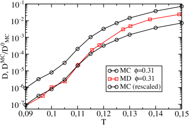
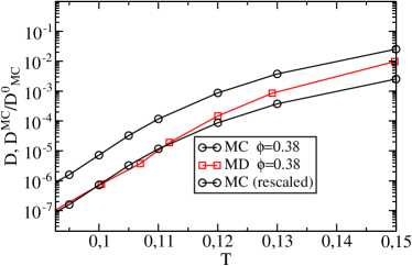
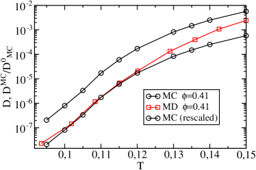
Figure 17: Comparison between the $MD$ and $MC$ diffusion coefficient at three different $\phi$ values. The MC data are also shown multiplied (by a common factor $0.1$) to better visualize the low $T$ overlap.

Since the microscopic time of the MC dynamics is not affected by temperature (being always fixed by the variance of the random displacements) it is interesting to consider the relation between $D$ and $E-E_{gs}$ also for $D^{MC}$, shown in Fig. 18 at the optimal network density $\phi=\phi=0.314$. Again, the slope of the curve has exponent four, but compared to the MD case, the region of validity of the power-law covers the entire range of $T$ studied, from very high $T$ (where the number of bonds is negligible) down to the lowest equilibrated temperature, covering more than 4 order of magnitude. The validity of the relation $D\sim(1-p_{b})^{4}$ extends up to high $T$, when the system is well above percolation and there is no evidence of a tetrahedral network (as shown in the structural data reported in Fig. 10 and 8). The extended validity of the power-law, with an exponent exactly equal to the valence of the model is highly suggestive and, in principle, very important for theoretical considerations, since it appears to cover either the region of temperature where liquid dynamics is observed, either the low $T$ states where signatures of slow dynamics (see Fig.11) are very well developed. The limit of validity of this finding needs to be carefully checked in other primitive models with different valence and with more realistic models of network forming liquids.

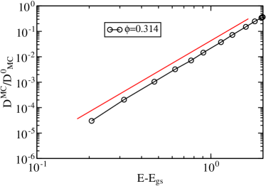
Figure 18: Relation between $D^{MC}$, normalized by the bare MD diffusion constant $D^{0}_{MC}$ and $E-E_{gs}$ for MC dynamics. Note that the MC data follow over more than five orders of magnitude a simple fourth-power law (full red line).

V Conclusions

Results presented in this manuscript cover several apparently distinct fields.

To start with, results presented here can be discussed in relation to the dynamic and thermodynamic properties of water. We have shown that the thermodynamic of the PMW includes, beside the compressibility anomalies reported beforeKolafa and Nezbeda (1987), also density anomalies (at much lower $T$). The source of the density anomalies is shown to be associated to the establishment of the bond network in the tetrahedral geometry. On cooling (along isochores) the energetic driving force which favors the formation of the bond, due to geometric constraints associated to the formation of the open tetrahedral structure, forces the pressure to increase and hence generating a density maximum state point. The simplicity of the PMW allows us also to clearly detect an optimal network density, at which the ground state of the system (i.e. the state in which each particle is involved in four bonds) can be closely approached. At this $\phi$ the $T$-dependence of the potential energy is the most pronounced, generating a minimum in the isothermal $\phi$ dependence. The presence of a minimum in $E(\phi)|_{T}$ is highly suggestive since it indicatesSciortino and Tartaglia (1997) the possibility of a liquid-liquid phase separation at $T$ lower than the one we have been able to equilibrate. We have also shown that at this optimal $\phi$, low $T$ dynamics slows down with the fourth power of the probability of broken bonds, i.e. the dominant component to dynamics arises from single particle motions, and specifically of the particles which happen to have all four bonds broken at the same time. We have also shown that, like in real water, diffusion anomalies are observed. At low $T$, the decrease of the diffusivity on increasing $\phi$ is reversed once the optimal network density is reached. For higher $\phi$, the progressive destruction of the bond network due to the increased packing fastens the dynamics. For even higher $\phi$, $D(\phi)$ resumes its standard decreasing behavior associated to the approach of the excluded volume glass transition. Diffusion and density anomalies in the PMW models are thus strongly related, similarly to what has been observed in more realistic models for waterErrington and Debenedetti (2001). The simplicity of the model is crucial in clarifying these aspects since the hard-core and square well interactions guarantee the absence of volumetric effects related to the $T$-dependence of the vibrational amplitudes.

A second interesting aspect of the presented results concerns the dynamics in network forming systems. The present study provides a complete characterization of the dynamics in the entire $(\phi-T)$ plane, from the smallest possible $\phi$ liquid state points up to the close packed state. From the reported data, the relative role of the energy and of the packing in controlling the dynamics stands up clearly. The isodiffusivity lines are essentially parallel to the $\phi$-axis (i.e. $T$ controlled) in the network low $\phi$ region and are essentially parallel to the $T$-axis (i.e. $\phi$ controlled) at larger $\phi$. Interesting enough, along isochores, low $T$ dynamics follows and Arrhenius law, the landmark of strong-glass forming behaviorAngell (1985); Debenedetti and Stillinger (2001). The Arrhenius law is foreseen by a $T$ region where dynamics has a strong $T$ dependence, compatible with a power-law dependence. In this power-law region the first signatures of caging in the mean square displacement are observed. Similar changes in the dynamics have been observed in previous studies of silicaHorbach and Kob (1999, 2001); Saika-Voivod et al. (2001), waterXu et al. (2005) and siliconSastry and Angell (2003). In particular, for the case of silica and water, it has been suggested that the region where dynamics start to feel the presence of energetic cages can be interpreted in terms of mode coupling theorySciortino et al. (1996); Sciortino and Kob (2001); Starr et al. (1999b); Fabbian et al. (1999b); Kob et al. (2002); Sciortino (2000); Horbach and Kob (1999, 2001).

Dynamics at the optimal network $\phi$ is particularly suggestive. Although in the present model, slowing down of the dynamics prevents equilibration of the supercooled liquid to very low $T$, at the lowest $T$ simulations the average number of bonds has gone up to 3.8 per particle. In this respect, further structural and dynamic changes are hard to foresee. This suggests that the Arrhenius behavior is retained down to $T=0$. Such speculation is reinforced by the numerical values of the activation energy of $D$ which is found to be $\approx 4u_{0}$, i.e. corresponding to the breaking of four bonds. This suggests that in network liquids, the limited valency imposed by the directional forces fixes a well defined energy of the local configuration and a discrete change of it which is reflected in the Arrhenius behavior. The presence of a limited valency and a well defined bond energy scale appears to be the key ingredient of the strong liquids behaviorMoreno et al. (2005). It is also worth to explore in future works the possibility that the optimal network density plays, in studies of one component systems, the same role as the reversibility windowChakravarty et al. (2005) in bulk alloy glasses. Connections with the concept of self-organization in network glassesHuerta and Naumis (2002) should also be pursued.

A further aspect of this work concerns the relative location between the liquid-gas spinodal and the kinetic arrest lines, whose shape is inferred by the study of the isodiffusivity lines. As in the short range SW modelZaccarelli et al. (2004); Foffi et al. (2005), the kinetic arrest lines ends in the right side of the spinodal, i.e. in the liquid phase. But differently from the SW case, the limited valency has shifted the right side of the spinodal to very small $\phi$ values, $\phi\lesssim 0.25$. Indeed, the limited valency effectively disfavors condensation of the liquid phase reducing the driving force for phase separation and making it possible to generate low packing fraction arrested states in the absence of phase separation, i.e homogeneous single phase stable in equilibrium, at low $T$Sciortino et al. (2005). The possibility to access low $T$ homogeneous supercooled states for $\phi>0.25$ characterized by a glassy dynamics, driven by the bonding energy as opposed to packing, confirms the findings of the zero-th order model with limited valency reported in Ref. Zaccarelli et al. (2005). The absence of geometric correlation between the bonding sites, the key ingredient of the maximum valency modelZaccarelli et al. (2005) is thus not crucial for the stabilization of the network. The role of the geometric constraint appears to be the reduction in the range of $\phi$ values where the fully bonded disordered state can be reached. Two different arrest mechanisms characterize the dynamics of network systems. Arrest due to the formation of energetic cages, with an arrest line which runs almost parallel to the $\phi$ axis, and arrest due to excluded volume effects, with an arrest line parallel to the $T$ axis. These two lines are reminiscent of the attractive and repulsive glass lines observed in short-range attractive colloidsFabbian et al. (1999b); Bergenholtz and Fuchs (1999); Dawson et al. (2001); Zaccarelli et al. (2002); Sciortino (2002). Connecting the results presented in this article with previous studies of network forming liquidsHorbach and Kob (1999); Sciortino et al. (1996), it is tempting to speculate that mode-coupling theory predicts satisfactory the shape in the $(\phi-T)$ plane of the dynamic arrest lines. Still, while in the region where excluded volume controls caging the relative error in the location of the glass line is limited , in the case in which bonding mechanism is dominant in generating arrest, the location of the MCT line can be significantly distant from the actual dynamic arrest line (technically located at $T=0$, being dynamics Arrhenius), due to the role of activated bond-breaking processes which offer a faster channel for the decay of the correlations. The evaluation of the MCT lines for the present model, in principle feasible within the site-site approach developed by Chong and GoetzeChong and Hirata (1998); Chong and Götze (2002) or within the molecular approach developed by SchillingSchilling and Scheidsteger (1997); Fabbian et al. (1999a) can help clarifying this issue.

The possibility of an intersection between the excluded volume arrest-line (starting at high $T$ from the HS glass packing fraction ) and the bond-controlled $T=0$ arrested line is particularly suggestive. The shape of the iso-diffusivity lines supports the possibility that the vertical repulsive glass line meets at a well defined $\phi$ the $T=0$ bond-controlled glass line. If this scenario is correct and general, one would conclude that the fragile and strong kinetic behavior is intimately connected to the dominant mechanism of arrest (fragile for excluded volume and strong for bonding) and, more interestingly, that strong behavior can only be observed when the interaction potential is such that less than six neighbors are present (i.e. in network forming systems). Indeed, only under these circumstances the suppression of the liquid-gas phase separation makes it possible to approach the $T=0$ bond-controlled glass line.

An additional comment concerns the relation between gel and glass arrest states. Results reported in this article confirm, one more, that in this class of models the geometric percolation line does not have any impact on the dynamic arrest, since at percolation the lifetime of the bond is still rather small. Only when the system is well inside the percolation region, the bond lifetime has slowed down significantly to affect all measurements of global connectivity with an intrinsic time scale shorter than the bond lifetime (as for example finite frequency shear viscosity). Indeed, already long time ago it was noted for the case of waterStanley and Teixeira (1980) that bond percolation is irrelevant to any thermodynamic or dynamic anomaly. More sophisticated models, incorporating bond-cooperativity or significant entropy contributions to bonding (as the case of polymeric gels) may reduce the differences between dynamic arrest states and percolationStarr and Sciortino (2005).

Despite the difference between percolation and arrest lines, if one consider the present model as a system of colloidal particles with sticky interactions, one would be led to call the arrested state at $0.3\lesssim\phi\lesssim 0.5$ a gel, led by the fact that the arrested state has a low $\phi$ open connected structure. Similarly, if one consider the PMW as a model for a network liquid, one would be led to name the same arrested state a network glass. While we cannot offer any resolution to this paradox with the present set of data, future work focusing on the shape of the wavevector dependence correlation functions and the resulting non ergodicity parameters can help clarifying this issue and confirm/dispute the hypothesis on the differences between gels and glasses recently proposedBergenholtz and Fuchs (1999); Zaccarelli et al. (2005); Foffi et al. (2005). At the present time, we can only call attention on the fact that a continuous change from energetic cages to excluded volume cages takes place on increasing $\phi$.

A final comment refers to the propensity of the system to form disordered arrested states. Despite the relevant amount of supercoolingVega and Monson (1998), in all studied state points where a network structure is present, we have not observed any sign of crystallization. The kinetic suppression of the crystallization phenomenon can be traced to the similar energy characterizing the crystal state and the fully bonded disordered state, vanishing the energetic driving force toward crystallization. The observed propensity to form gel states as opposed to crystalline states manifested by the studied model (which can be seen also as a model for short-range sticky colloid particles as well as globular proteins with aeolotopic interactionsLomakin et al. (1999)) may well explain the difficulty of crystallizing some class of proteins. It also warn us about the relevance of the dynamic arrest phenomenon in the future attempts to build a colloidal diamond photonic crystal, made of particles with short-ranged patchy interactions.

VI Acknowledgements

We thank E. Zaccarelli. We acknowledge support from MIUR-FIRB and CRTN-CT-2003-504712.

VII Appendix: An event-driven algorithm for hard spheres with patches.

In an event driven (ED) algorithm, events such as times of collisions between particles and cell crossing have to be taken into account. All these events have to be ordered. Code must be written in such a way that locating the next event and insertion/deletion of new events have to be performed efficiently. In literature, several ED algorithms for simulating hard-sphere systems exist and several propositions on how to handle such events efficiently have been reported. One elegant approach, proposed twenty years ago by Rapaport Rapaport (2004), arranges events into an ordered binary tree (calendar of events) so that insertion, deletion and retrieving of events can be done with an efficiency $O(\log N)$, $O(1)$ and $O(\log N)$ respectively, where $N$ is the number of events in the calendar. We adopted this solution to handle the events calendar in our simulation, adding only a redefinition of event time in order to avoid round-off problems which are found when extremely long simulation runs are performed.

VII.1 Motion of rigid bodies

The orientation of a rigid body can be conveniently represented by the $3$ column eigenvectors ${\bf u}_{i}$ (with $i=1,2,3$) of the inertia tensor expressed in the laboratory reference system. These vectors form an orthogonal set and can be arranged in a matrix ${\bf R}$, i.e.

$${\bf R}={}^{t}({\bf u}_{0}\ {\bf u}_{1}\ {\bf u}_{2})$$ (11)

where ${}^{t}A$ indicates the transpose of the matrix $A$. This matrix is such that if ${\bf x}$ are the coordinates of the laboratory reference system and ${\bf x^{\prime}}$ are the coordinates of the rigid body reference system, it turns out that:

$${\bf x}^{\prime}={\bf R}{\bf x}$$ (12)

In what follows, we assume that the three eigenvalues of the inertia tensor are all equal to $I$. Naming ${\bf w}=(w_{x},w_{y},w_{z})$ the angular velocity of a free rigid body, the matrix ${\bf\Omega}$ is defined as

$${\bf\Omega}=\begin{pmatrix}0&-w_{z}&w_{y}\cr w_{z}&0&-w_{x}\cr-w_{y}&w_{x}&0\end{pmatrix}$$ (13)

Knowing the orientation at time $t=0$, the orientation ${\bf R}(t)$ at time $t$ is: Landau and Lifshitz (1960); Goldstein (1980):

$${\bf R}(t)={\bf R}(0)({\bf I}+{\bf M})$$ (14)

where ${\bf M}$ is the following matrix:

$${\bf M}=-\frac{\sin(wt)}{w}{\bf\Omega}+\frac{1-\cos(wt)}{w^{2}}{\bf\Omega}^{2}$$ (15)

and $w=\|{\bf w}\|$. Note that if $w=0$ then ${\bf R}(t)={\bf R}(0)$. To derive Eq. 14, consider that:

$${}^{t}R(t) = ({\bf u}_{1}(t)\ {\bf u}_{2}(t)\ {\bf u}_{3}(t))$$

$$= ({}^{t}({\bf I}+{\bf M}){\bf u}_{1}\ {}^{t}({\bf I}+{\bf M}){\bf u}_{2}\ {}^{t}({\bf I}+{\bf M}){\bf u}_{3}\ )$$

where we remember that ${\bf u}_{i}$ are column vectors. Hence, if ${\bf w}=w{\bf\hat{n}}$, we have after some algebra:

$${\bf u}_{i}(t)={\bf u}_{i}\cdot{\bf\hat{n}}\;{\bf\hat{n}}+\cos(wt)({\bf u}_{i}-{\bf\hat{n}}\cdot{\bf u}_{i}\>{\bf\hat{n}})+\sin(wt)\;{\bf\hat{n}}\times{\bf u}_{i}$$ (17)

that is the so-called Rodriguez’s formula or Rotation formula, i.e. a rotation of an angle $wt$ around the axis ${\hat{n}}$. To conclude if one has to update position and orientation of a rigid body, that is freely moving, this can be accomplished doing:

$${\bf x}(t)={\bf x}(0)+{\bf v}t$$ (18a)

$${\bf R}(t)={\bf R}(0)({\bf I}+{\bf M})$$ (18b)

where ${\bf x}(t)$ is the position of the center of mass of the rigid body at time $t$ and $\bf v$ is its velocity.

VII.2 Hard-Sphere with interacting patches

In the present model, each particle is modeled as an hard sphere with $n$ spherical patches arranged in fixed site locations. In the present case, the site-site interaction is a SW potential,

$$u_{SW}=\begin{cases}-u_{0}&\hbox{if}\ \ r<\delta\cr 0&\hbox{otherwise}\cr\end{cases}$$ (19)

where $\delta$ and $u_{0}$ are the width and the depth of the SW . For the following discussion, the SW interaction can be visualized as a sphere of diameter $\delta$ centered on the site location. Similarly, one can visualize the particle as a rigid body composed by the hard-sphere joined to the spheres located on the sites. In what follows, we identify a particle with the resulting surface. Defining distance $d_{AB}$ between two particles $A$ and $B$ as the shortest line connecting two points on distinct particles, i.e.

$$d_{AB}=\min_{i_{A},i_{B}}{d_{i_{A}i_{B}}}$$ (20)

where $i_{A},i_{B}\in\{0,\dots n\}$ and $0$ labels the hard sphere, $1\dots n$ label the $n$ spherical patches and $d_{i_{A}i_{B}}$ is the distance between the two spherical patches $i_{A}$ and $i_{B}$.

VII.3 Prediction of time-of-collision

VII.3.1 Finding the contact time

We separate the collisions between two particles in the hard-sphere part of the potential and the site-site interaction part. The time of collision $t_{hs}$ between the hard sphere cores can be evaluated as usual Rapaport (2004) . The smallest time of collision among all $n^{2}$ spherical patch pairs is $t_{st}$. Time of collision of the two particles is

$$t_{c}=\min\{t_{hs},t_{st}\}$$ (21)

To find the time-of-collision of two interacting patches we assume that it is possible to bracket it. I.e., we assume (see further subsections) that the time of collision $t_{st}$ is such that $t_{1}<t_{st}<t_{2}$ where the product $d(t_{1})d(t_{2})<0$. Thus, the “exact“ time of collision is provided by the root of the following equation:

$$\|r_{i_{A}}(t)-r_{i_{B}}(t)\|=\delta$$ (22)

where $r_{i_{A}}$ and $r_{i_{B}}$ are the two site locations.

VII.3.2 Linked lists and Centroids

As described in Rapaport (2004) to speed up a ED molecular dynamics of hard spheres one can use linked lists. For a system of $N$ identical particles inside a cubic box of edge $L$, we define the “centroid” Donev et al. (2005a, b) as the smallest sphere that contains the particle (the HS and the spherical patches). Linked lists of centroids may be quite useful to reduce the number of objects to check for possible collisions and in addition they can be used to restrict the time interval within which searching for the collision. We divide the box into $M^{3}$ cells so that into each cell contains at most one centroid. After that we build the linked lists of these centroids and handle these lists as done in a usual ED molecular dynamics of hard spheres Rapaport (2004). This means that whenever an object cross a cell boundary one has to remove such an object from the cell the particle is coming from and add this object to the cell where it’s going to.

Now consider that one has to predict all the possible collisions of a given particle, which is inside a certain cell $m$. As for the hard spheres case we take into account only the particles inside the adjacent cells (see Rapaport (2004) for more details) and we predict the times of collisions with these objects. Consider now two particles $A$ and $B$ at time $t=0$ and their centroids $C_{A}$ and $C_{B}$. Three possible cases arise:

1. $C_{A}$ and $C_{B}$ do not overlap and, evaluating their trajectory no collision between the two centroids is predicted. In this case $A$ and $B$ won’t collide as well.

2. $C_{A}$ and $C_{B}$ do not overlap but they will collide: in this case, we calculate two times $t_{1}$ and $t_{2}$, bracketing the possible collision between $A$ and $B$: $t_{1}$ is defined as the time when the two centroids collide and start overlapping and $t_{2}$ is the time when the two spheres have completely crossed each other and do not overlap any longer.

3. $C_{A}$ and $C_{B}$ overlap: in this case $t_{1}\equiv 0$ and $t_{2}$ is defined as the time at which the two centroids stop overlapping.

VII.3.3 Fine temporal bracketing of the contact time

Here we show how a refined bracketing of solution of Eq. 22 can be accomplished. First of all we give an overestimate of the rate of variation of the distance between two patches $i_{A}$ and $i_{B}$, that is:

$$\dot{d}_{i_{A}i_{B}}(t) = \frac{d}{dt}\left(\|{\bf r}_{i_{A}}-{\bf r}_{i_{B}}\|-\delta\right)$$ (23)

$$\leq \frac{{\bf\dot{r}}_{i_{A}i_{B}}\cdot{\bf r}_{i_{A}i_{B}}}{\|{\bf r}_{i_{A}i_{B}}\|}\leq\|{\bf v}_{i_{A}i_{B}}\|$$ (24)

$$= \|{\bf V}_{AB}+{\bf\omega}_{A}\times({\bf r}_{i_{A}}-{\bf R}_{A})-{\bf\omega}_{B}\times({\bf r}_{i_{B}}-{\bf R}_{B})\|$$ (25)

$$\leq \|{\bf V}_{AB}\|+\|{\bf\omega}_{A}\|L_{A}+\|{\bf\omega}_{B}\|L_{B}=\dot{d}^{max}_{i_{A}i_{B}}$$ (26)

where the dot indicates the derivation with respect to time, ${\bf r}_{i_{A}}$, ${\bf r}_{i_{B}}$ are the positions of the two sites with respect to laboratory reference system, ${\bf v}_{i_{A}i_{B}}$, is the relative velocity of the two sites, ${\bf V}_{AB}$ is the relative velocity between the centers of mass of the two particles, ${\bf R}_{A}$ and ${\bf R}_{B}$ are the positions of their centers of mass and

$$L_{A}\geq\max_{{\bf r}^{\prime}\in A}\{\|{\bf r}^{\prime}-{\bf R}_{A}\|\}$$ (27a)

$$L_{B}\geq\max_{{\bf r}^{\prime}\in B}\{\|{\bf r}^{\prime}-{\bf R}_{B}\|\}$$ (27b)

Having calculated an overestimate of $\dot{d}_{i_{A}i_{B}}(t)$ we can evaluate an overestimate of $\dot{d}_{AB}$ that we call $\dot{d}_{max}$:

$$\dot{d}_{max}=\max_{i_{A}i_{B}}\{\dot{d}_{i_{A}i_{B}}^{max}\}$$ (28)

Using Eq. (28) we can easily find an efficient strategy to bracket the solution. In fact the following algorithm can be used:

1. Evaluate the distances between all sites that may interact $\{d_{i_{A}i_{B}}(t)\}_{i_{A}i_{B}}$ at time $t$ (starting the first time from $t_{1}$).

2. Choose a time increment $\Delta t$ as follows:

   $$\Delta t=\begin{cases}\frac{d_{AB}(t)}{\dot{d}_{max}},&\hbox{if}\>d_{AB}(t)>\epsilon_{f}\hbox{;}\cr\frac{\epsilon_{d}}{\dot{d}_{max}},&\hbox{otherwise.}\cr\end{cases}$$ (29)

   where the two arbitrary parameters $\epsilon_{d}$ and $\epsilon_{f}$ satisfy $\epsilon_{d}<\epsilon_{f}\ll\min\{L_{A},L_{B}\}$.

3. Evaluate the distances at time $t+\Delta t$.

4. If for at least one pair of patches $(i_{A},i_{B})$ we find that the product $d_{i_{A}i_{B}}(t+\Delta t)d_{i_{A}i_{B}}(t)<0$ we have bracketed a solution. We then find the collision times and the collision points solving Eq. (22) for all pairs. Choose the smallest collision time and terminate.

5. if pairs of patches are such that $0<|d_{i_{A}i_{B}}(t+\Delta t)|<\epsilon_{d}$ and $0<|d_{i_{A}i_{B}}(t)|<\epsilon_{d}$, for each of these pairs evaluate the distance $d_{i_{A}i_{B}}(t+\Delta t/2)$, perform a quadratic interpolation of these $3$ points $(t,d_{i_{A}i_{B}}(t))$, $(t+\Delta t/2,d_{i_{A}i_{B}}(t+\Delta t/2)$, $(t+\Delta t,d_{i_{A}i_{B}}(t+\Delta t)$ and find if the resulting parabolas have zeros. If yes refine the smallest zero solving again Eq. (22) for all these pairs.

6. Increment time by $\Delta t$, i.e.

   $$t\rightarrow t+\Delta t$$ (30)

7. Go to step 1, if $t<t_{2}$.

If two particles undergo a “grazing” collision, i.e. a collision where the modulus of the distance stays smaller than $\epsilon_{d}$ during the collision, the collision could not be located by the previous algorithm due to failure of the quadratic interpolation. We have chosen to work with $\epsilon_{d}\approx 10^{-6}$. For such a choice, we have not observed grazing collisions during the simulation runs (which would appear in the conservation of the energy).

The basic algorithm can be improved with simple optimizations. For example one can calculate $\dot{d}_{i_{A}i_{B}}^{max}$ as follows:

$$\dot{d}_{i_{A}i_{B}}^{max}=\|{\bf V}_{AB}\|+\|{\bf\omega}_{A}\|L_{i_{A}}+\|{\bf\omega}_{B}\|L_{i_{B}}$$ (31)

where

$$L_{i_{A}}=\|{\bf r_{i_{A}}}^{\prime}-{\bf R}_{A}\|$$ (32a)

$$L_{i_{B}}=\|{\bf r_{i_{B}}}^{\prime}-{\bf R}_{B}\|$$ (32b)

and if $d_{AB}(t)>\epsilon_{f}$ the time increment can be evaluated in the following optmized way:

$$\Delta t=\min_{i_{A}i_{B}}\{d_{i_{A}i_{B}}(t)/d_{i_{A}i_{B}}^{max}\}$$ (33)

VII.4 Collision of two particles

At the collision time, one has to evaluate the new velocities of centers of mass and the new angular velocities. If ${\bf x}_{C}$ is the contact point then the velocities after the collision can be evaluated as follows:

$${\bf v}_{A}\rightarrow{\bf v}_{A}+m_{A}^{-1}\Delta p_{AB}{\bf\hat{n}}$$ (34a)

$${\bf v}_{B}\rightarrow{\bf v}_{B}-m_{B}^{-1}\Delta p_{AB}{\bf\hat{n}}$$ (34b)

$${\bf w}_{A}\rightarrow{\bf w}_{A}+\Delta p_{AB}I_{A}^{-1}({\bf r}_{A}-{\bf x}_{C})\times{\bf\hat{n}}$$ (34c)

$${\bf w}_{B}\rightarrow{\bf w}_{B}-\Delta p_{AB}I_{B}^{-1}({\bf r}_{B}-{\bf x}_{C})\times{\bf\hat{n}}$$ (34d)

where ${\bf\hat{n}}$ is a unit vector perpendicular to both surfaces at the contact point ${\bf x}_{C}$, $I_{A}$, $I_{B}$ are the moments of inertia of the two colliding sticky particles, $m_{A}$, $m_{B}$ their masses and the quantity $\Delta p_{AB}$ depends on the type of the collision. If we define

$$v_{c}=({\bf v}_{A}+{\bf w}_{A}\times{\bf(}{\bf x}_{C}-{\bf r}_{A})-{\bf v}_{B}-{\bf w}_{B}\times{\bf(}{\bf x}_{C}-{\bf r}_{B}))\cdot{\bf\hat{n}}$$ (35)

If the collision occurring between particles is an hard-core collision, one has:

$$\Delta p_{AB}=-2v_{c}$$ (36)

if the collision occurred between two spherical patches already bonded (i.e. prior the collision the distance between the two sites is $<\delta$ one has:

$$\Delta p_{AB}=\begin{cases}-2v_{c}&\hbox{if}\ \ v_{c}^{2}<2u_{0}/M_{red}\cr-v_{c}+\sqrt{v_{c}^{2}-2u_{0}/M_{red}}&\hbox{otherwise}\end{cases}$$ (37)

where

$$M_{red}^{-1}=m_{A}^{-1}+m_{B}^{-1}+I_{A}^{-1}\|({\bf r}_{A}-{\bf x}_{C})\times{\bf\hat{n}}\|+I_{B}^{-1}\|({\bf r}_{B}-{\bf x}_{C})\times{\bf\hat{n}}\|$$ (38)

Finally if the collision occurs between two patches that are not bonded (i.e. the distance between the two sites is $>\delta$ prior the collision) we have:

$$\Delta p_{AB}=-v_{c}+\sqrt{v_{c}^{2}-2u_{0}/M_{red}}$$ (39)

VIII Appendix: Evaluating the pressure

VIII.1 Evaluating the pressure in the ED code

We define the quantity:

$$\Delta A_{\alpha\beta}(t)=V\int_{0}^{t}{\cal P}_{\alpha\beta}(t^{\prime})dt^{\prime}$$ (40)

where ${\cal P}_{\alpha\beta}$ is the molecular pressure tensor,

$${\cal P}_{\alpha\beta}V=\sum_{i=1}^{N}M_{i}V_{i\alpha}V_{i\beta}+\sum_{i=1}^{N}\sum_{j>i}^{N}F_{ij\alpha}(R_{i\beta}-R_{j\beta})$$ (41)

The sums in the previous expression involve components (denoted by greek letters), ${\vec{V}}_{i}$, ${\vec{R}}_{i}$ and ${\vec{F}}_{ij}$, which are the velocity, the position of center of mass of $i$-th particle (mass $M_{i}$) and the total force acting between particle $i$ and $j$ respectively.

In the presence of impulsive forces, the stress tensor defined in Eq. (41) is not well defined, while the integral in Eq. (40) is well defined. Consider the time interval $(t,t+\Delta t)$. During this interval the quantity $\Delta A_{\alpha\beta}(t)$ will vary due to the collisions occurring between particles. The variation $\delta A(t)$ of $\Delta A(t)$, is:

$$\delta A_{\alpha\beta}(t)=\sum_{i}^{N}M_{i}V_{i\alpha}V_{i\beta}\delta t+R_{i\alpha}\delta P_{i\beta}$$

where $\delta t$ is the time elapsed from last collision occurred in the system and $\delta{\bf P}_{i}$ is the variation of momentum of particle $i$ after the collision, i.e.

$$\delta P_{i\alpha}=\Delta p_{AB}{\hat{n}}_{\alpha}$$ (42)

where $\Delta p_{AB}$ is the quantity defined in Eq. (35).

From $\Delta A_{\alpha\beta}(t)$ and $\Delta A_{\alpha\beta}(t+\Delta t)$ the average pressure over the interval $\Delta t$ can be evaluated as follows:

$$P=\frac{1}{3V}\sum_{\alpha}\frac{\Delta A_{\alpha\alpha}(t+\Delta t)-\Delta A_{\alpha\alpha}(t)}{\Delta t}$$ (43)

VIII.2 Evaluating $P$ in MC

In the analysis of MC configurations, pressure has been calculated as sum of three contributions. A trivial kinetic contribution, equal to $nk_{B}T$; a positive HS contribution, which requires the evaluation of the hard sphere radial distribution function $g_{{}_{HS}}(r)$ at distance $\sigma$ and a negative contribution arising from the SW interaction, which requires both the evaluation of the $H-LP$ radial distribution function $g_{{}_{H-LP}}(r)$ at distance $\delta$ as well as the evaluation of $<R_{H-LP}(r)>$. For a pair of $H$ and $LP$ sites whose distance is $r$, the quantity $R_{H-LP}$ is defined as the projection of the vector joining the centers of the two particles associated to the two sites along the direction of the unitary vector joining the two sites. The ensemble average $<...>$ is performed over all pairs of $H$ and $LP$ sites at relative distance $r$ Kolafa and Nezbeda (1987).

The resulting expression for $P$ is

$$P=nk_{B}T(1+\frac{4\phi}{~{}}~{}~{}~{}~{}~{}$$ (44)

$$\left[g_{{}_{HS}}(\sigma)-8\frac{\delta^{2}}{\sigma^{3}}(1-e^{-1/T})<R_{H-LP}(\delta)>g_{{}_{H-LP}}(\delta)\right])$$

.

References

- Kolafa and Nezbeda (1987) J. Kolafa and I. Nezbeda, Mol. Phys. 61, 161 (1987).
- Lomakin et al. (1999) A. Lomakin, N. Asherie, and G. B. Benedek, Proc. Natl. Acad. Sci. 96, 9465 (1999).
- Sear (1999) R. P. Sear, J. Chem. Phys. 111, 4800 (1999).
- Kern and Frenkel (2003) N. Kern and D. Frenkel, J.Chem Phys. 118, 9882 (2003).
- Manoharan et al. (2003) V. N. Manoharan, M. T. Elsesser, and D. J. Pine, Science 301, 483 (2003).
- Yethiraj and van Blaaderen (2003) A. Yethiraj and A. van Blaaderen, Nature 421, 513 (2003).
- Zaccarelli et al. (2005) E. Zaccarelli, S. V. Buldyrev, E. L. Nave, A. J. Moreno, I. Saika-Voivod, F. Sciortino, and P. Tartaglia, Phys. Rev Lett. 94, 218301 (2005).
- Moreno et al. (2005) A. J. Moreno, S. V. Buldyrev, E. L. Nave, I. Saika-Voivod, F. Sciortino, P. Tartaglia, and E. Zaccarelli, Phys. Rev. Lett. 95, 157802 (2005).
- Speedy and Debenedetti (1994) R. J. Speedy and P. G. Debenedetti, Mol. Phys. 81, 1293 (1994).
- Speedy and Debenedetti (1995) R. J. Speedy and P. G. Debenedetti, Mol. Phys. 86, 1375 (1995).
- Speedy and Debenedetti (1996) R. J. Speedy and P. G. Debenedetti, Mol. Phys. 88, 1293 (1996).
- Bratko et al. (1985) D. Bratko, L. Blum, and A. Luzar, J. Chem. Phys. 83, 6367 (1985).
- Nezbeda et al. (1989) I. Nezbeda, J. Kolafa, and Y. Kalyuzhnyi, Mol. Phys. 68, 143 (1989).
- Nezbeda and Iglesias-Silva (1990) I. Nezbeda and G. Iglesias-Silva, Mol. Phys. 69, 767 (1990).
- Vega and Monson (1998) C. Vega and P. A. Monson, J. Chem. Phys. 109, 9938 (1998).
- Wertheim (1984a) M. S. Wertheim, J. Stat. Phys. 35, 19 (1984a).
- Wertheim (1984b) M. S. Wertheim, J. Stat. Phys. 35, 35 (1984b).
- Ghonasci and Chapman (1993) D. Ghonasci and W. G. Chapman, Mol. Phys. 79, 291 (1993).
- Sear and Jackson (1996) R. P. Sear and G. Jackson, J. Chem. Phys. 105, 1113 (1996).
- Duda et al. (1998) Y. Duda, C. J. Segura, E. Vakarin, M. F. Holovko, and W. G. Chapman, J. Chem. Phys. 108, 9168 (1998).
- Peery and Evans (2003) T. B. Peery and G. T. Evans, J. Chem Phys. 118, 2286 (2003).
- Kalyuzhnyi and Cummings (2003) Y. V. Kalyuzhnyi and P. T. Cummings, J. Chem Phys. 118, 6437 (2003).
- Vlcek et al. (2003) L. Vlcek, J. Slovak, and I. Nezbeda, Mol. Phys. 101, 2921 (2003).
- Glotzer (2004) S. C. Glotzer, Science 306, 419 (2004).
- Zhang and Glotzer (2004) Z. L. Zhang and S. C. Glotzer, Nano Lett. 4, 1407 (2004).
- Sciortino (2002) F. Sciortino, Nature Materials 1, 145 (2002).
- Gado and Kob (2005) E. D. Gado and W. Kob, cond-mat/0507085 (2005).
- Zaccarelli et al. (2005) E. Zaccarelli et al., in preparation (2005).
- Sciortino et al. (1997a) F. Sciortino, P. H. Poole, U. Essmann, and H. E. Stanley, Phys. Rev. E 55, 727 (1997a).
- Poole et al. (1992) P. H. Poole, F. Sciortino, U. Essmann, and H. E. Stanley, Nature 360, 324 (1992).
- Poole et al. (1993) P. H. Poole, F. Sciortino, U. Essmann, and H. E. Stanley, Phys. Rev. E 48, 3799 (1993).
- Yamada et al. (2002) M. Yamada, S. Mossa, H. E. Stanley, and F. Sciortino, Phys. Rev. Lett. 88, 1 (2002).
- Poole et al. (2005) P. Poole, I. Saika-Voivod, and F. Sciortino, J. Phys.: Condens. Matter 17, L431 (2005).
- Paschek (2005) D. Paschek, Phys. Rev. Lett. 94, 217802 (2005).
- Brovchenko et al. (2005) I. Brovchenko, A. Geiger, and A. Oleinikova, J. Chem. Phys. 123, 4515 (2005).
- Hansen and McDonald (1986) J. P. Hansen and I. R. McDonald, Theory of simple liquids (Academic, New York, 1986).
- Pagan and Gunton (2005) D. L. Pagan and J. D. Gunton, J. Chem. Phys. 122, 4515 (2005).
- Sciortino (2005) F. Sciortino, J. Phys.: Condens. Matter 17, 32 (2005).
- Stillinger and Rahman (1974) F. H. Stillinger and A. Rahman, J. Chem. Phys. 60, 1545 (1974).
- Hill (1987) T. L. Hill, An Introduction to Statistical Thermodynamics (Dover Pubns, 1987).
- Coniglio et al. (2004) A. Coniglio, L. D. Arcangelis, E. D. Gado, A. Fierro, and N. Sator, J. Phys.: Condens. Matter 16, S4831 (2004).
- Stauffer and Aharony (1992) D. Stauffer and A. Aharony, Introduction to Percolation Theory (Taylor and Francis, London, 1992), 2nd ed.
- Sciortino et al. (1996) F. Sciortino, P. Gallo, P. Tartaglia, and S. H. Chen, Phys. Rev. E 54, 6331 (1996).
- Gallo et al. (1996) P. Gallo, F. Sciortino, P. Tartaglia, and S. H. Chen, Phys. Rev. Lett. 76, 2730 (1996).
- Starr et al. (1999a) F. W. Starr, F. Sciortino, and H. E. Stanley, Phys. Rev. E 60, 6757 (1999a).
- Fabbian et al. (1999a) L. Fabbian, A. Latz, R. Schilling, F. Sciortino, P. Tartaglia, and C. Theis, Phys. Rev. E 60, 5768 (1999a).
- Sciortino et al. (1997b) F. Sciortino, L. Fabbian, S. H. Chen, and P. Tartaglia, Phys. Rev. E 56, 5397 (1997b).
- Fabbian et al. (1998) L. Fabbian, F. Sciortino, F. Thiery, and P. Tartaglia, Phys. Rev. E 57, 1485 (1998).
- Horbach and Kob (1999) J. Horbach and W. Kob, Phys. Rev. B 60, 3169 (1999).
- Saika-Voivod et al. (2001) I. Saika-Voivod, P. H. Poole, and F. Sciortino, Nature 412, 514 (2001).
- Xu et al. (2005) L. Xu, P. Kumar, S. V. Buldyrev, S.-H. Chen, P. H. Poole, F. Sciortino, and H. E. Stanley, Proc. Natl. Acad. Sci. 102, XXX (2005).
- Scala et al. (2000) A. Scala, F. Starr, E. La Nave, F. Sciortino, and H. E. Stanley, Nature 406, 166 (2000).
- Tölle (2001) A. Tölle, Rep. Prog. Phys. 64, 1473 (2001).
- Foffi et al. (2002) G. Foffi, K. A. Dawson, S. V. Buldrey, F. Sciortino, E. Zaccarelli, and P. Tartaglia, Phys. Rev. E 65, 050802 (2002).
- Zaccarelli et al. (2002) E. Zaccarelli, G. Foffi, K. A. Dawson, S. V. Buldrey, F. Sciortino, and P. Tartaglia, Phys. Rev. E 66, 041402 (2002).
- Sciortino et al. (2004) F. Sciortino, S. Mossa, E. Zaccarelli, and P. Tartaglia, Phys. Rev. Lett. 93, 1 (2004).
- Dawson et al. (2001) K. Dawson, G. Foffi, M. Fuchs, F. Sciortino, M. Sperl, P. Tartaglia, T. Voigtmann, and E. Zaccarelli, Phys. Rev. E 63, 011401 (2001).
- Teixeira (1990) J. Teixeira, Correlations and Connectivity (Kluver Academic Publishers, Dordrecht, 1990), h.e. stanley and n. ostrowsky ed.
- Stanley and Teixeira (1980) H. E. Stanley and J. Teixeira, J. Chem. Phys. 73, 3404 (1980).
- Starr and Sciortino (2005) F. Starr and F. Sciortino, preprint (2005).
- Sciortino and Tartaglia (1997) F. Sciortino and P. Tartaglia, Phys. Rev. Lett. 78, 2385 (1997).
- Errington and Debenedetti (2001) J. R. Errington and P. G. Debenedetti, Nature 409, 318 (2001).
- Angell (1985) C. A. Angell, J. Non-Cryst. Solids 73, 1 (1985).
- Debenedetti and Stillinger (2001) P. G. Debenedetti and F. H. Stillinger, Nature (London) 410, 259 (2001).
- Horbach and Kob (2001) J. Horbach and W. Kob, Phys. Rev. E 64, 041503 (2001).
- Sastry and Angell (2003) S. Sastry and C. A. Angell, Nature Materials 2, 739 (2003).
- Sciortino and Kob (2001) F. Sciortino and W. Kob, Phys. Rev. Lett. 86, 648 (2001).
- Starr et al. (1999b) F. W. Starr, S. Harrington, F. Sciortino, and H. E. Stanley, Phys. Rev. Lett. 82, 3629 (1999b).
- Fabbian et al. (1999b) L. Fabbian, W. Götze, F. Sciortino, P. Tartaglia, and F. Thiery, Phys. Rev. E 59, 1347 (1999b).
- Kob et al. (2002) W. Kob, M. Nauroth, and F. Sciortino, J. Non-Cryst. Solids 307, 181 (2002).
- Sciortino (2000) F. Sciortino, Chemical Physics pp. 307–314 (2000).
- Chakravarty et al. (2005) S. Chakravarty, D. G. Georgiev, P. Boolchand, and M. Micoulaut, J. Phys.: Condens. Matter 17, L1 (2005).
- Huerta and Naumis (2002) A. Huerta and G. G. Naumis, Phys. Rev. B 66, 184204 (2002).
- Zaccarelli et al. (2004) E. Zaccarelli, F. Sciortino, S. V. Buldyrev, and P. Tartaglia, Short-ranged attractive colloids: What is the gel state? (Elsevier, Amsterdam, 2004), p. 181, in Unifyng Concepts in Granular Media and Glasses, A. Coniglio, A. Fierro, H.J. Herrmann and M. Nicodemi ed.
- Foffi et al. (2005) G. Foffi, C. De Michele, F. Sciortino, and P. Tartaglia, Phys. Rev. Lett. 94, 078301 (2005).
- Sciortino et al. (2005) F. Sciortino, S. Buldyrev, C. De Michele, N. Ghofraniha, E. La Nave, A. Moreno, S. Mossa, P. Tartaglia, and E. Zaccarelli, Comp. Phys. Comm. 169, 166 (2005).
- Bergenholtz and Fuchs (1999) J. Bergenholtz and M. Fuchs, Phys. Rev. E 59, 5706 (1999).
- Chong and Hirata (1998) S. H. Chong and F. Hirata, Phys. Rev. E 58, 6188 (1998).
- Chong and Götze (2002) S. H. Chong and W. Götze, Phys. Rev. E 65, 041503 (2002).
- Schilling and Scheidsteger (1997) R. Schilling and T. Scheidsteger, Phys. Rev. E 56, 2932 (1997).
- Foffi et al. (2005) G. Foffi, C. De Michele, F. Sciortino, and P. Tartaglia, J. Chem. Phys. 122, 4903 (2005).
- Rapaport (2004) D. C. Rapaport, The Art of Molecular Dynamics Simulation (Cambridge University Press, 2004).
- Landau and Lifshitz (1960) L. Landau and E. Lifshitz, Course of theoretical physics, vol. 1, Mechanics (Pergamon Press, 1960).
- Goldstein (1980) H. Goldstein, Classical Mechanics (Addison Wesley, 1980), 2nd ed.
- Donev et al. (2005a) A. Donev, F. H. Stillinger, and S. Torquato, J. Comp. Phys 202, 737 (2005a).
- Donev et al. (2005b) A. Donev, F. H. Stillinger, and S. Torquato, J. Comp. Phys 202, 765 (2005b).