Effects of Preference for Attachment to Low-degree Nodes on the Degree Distributions of a Growing Directed Network and a Simple Food-Web Model

Abstract

We study the growth of a directed network, in which the growth is constrained by the cost of adding links to the existing nodes. We propose a new preferential-attachment scheme, in which a new node attaches to an existing node $i$ with probability $\Pi(k_{i})\propto k_{i}^{-1}$, where $k_{i}$ is the number of outgoing links at $i$. We calculate the degree distribution for the outgoing links in the asymptotic regime ($t\rightarrow\infty$), $n_{k}^{*}$, both analytically and by Monte Carlo simulations. The distribution decays like $k\mu^{k}/\Gamma(k)$ for large $k$, where $\mu$ is a constant. We investigate the effect of this preferential-attachment scheme, by comparing the results to an equivalent growth model with a degree-independent probability of attachment, which gives an exponential outdegree distribution. Also, we relate this mechanism to simple food-web models by implementing it in the cascade model. We show that the low-degree preferential-attachment mechanism breaks the symmetry between in- and outdegree distributions in the cascade model. It also causes a faster decay in the tails of the outdegree distributions for both our network growth model and the cascade model.

I Introduction

Many real-world networks that have been studied recently, such as the internet, the World Wide Web, and social relations have a scale-free structure, whose degree distribution, $P(l)$, follows a power law for large $l$, the number of links connecting to a single node. A scale-free network can be constructed using a preferential-attachment mechanism in which a new node attaches to an existing node, $i$, which has $l_{i}$ links with a probability $\Pi(l_{i})=l_{i}/\sum_{j}{l_{j}}$ Barabasi:1999 . This form of preferential attachment means that the highly connected nodes attract more new nodes than the others, and it explains the structure of networks like the internet, in which a connection is favorable for both connected nodes, and where links are undirected. Growth according to this mechanism leads to self-organization into a scale-free structure Barabasi:1999 ; Barabasi:2002 ; Dorogovtsev:2000 ; Krapivsky:2000 ; Krapivsky:2001 .

In this paper, we propose a new preferential-attachment scheme for growing directed networks Dorogovtsev:2001 ; Rodgers:2001 , in which new nodes prefer to attach to existing nodes with lower degree. Such a mechanism could play a role in some transportation networks Garlaschelli:2003 ; Banavar:1999 such as food webs Drossel:2002 ; Martinez:2002 ; Montoya:2003 ; McKane-Rev or power-grids Amaral:2000 ; Albert:2004 , which can be considered directed. The links in such networks transport some sort of resource to “feed” the nodes. Each node gets resources only by feeding on another one. (The initial nodes can be considered as sources.) We take the direction of the resource flow as the direction of the link. Therefore, an outgoing link transports resources from a “prey” node to a “predator” node. If there is more than one predator that feeds on a prey node, then the resources supplied by the prey have to be shared by the predators. This implies that for a conventional growth model, the attractiveness of a node in such a network should increase with the number of its incoming links (indegree), and decrease with the number of its outgoing links (outdegree). In other words, the cost of adding links to an existing node should increase due to limited capacity, as the number of nodes that feed on it increases. This cost puts a constraint on the growth of the network Amaral:2000 . A good example of such a system, the world-wide airport network, is studied in Ref.  Guimera:2004 .

Therefore, we propose a new growth scheme, in which a new node attaches to an existing node, $i$, with probability $\Pi(k^{\prime}_{i},k_{i})\propto(k^{\prime}_{i}/k_{i})^{\gamma}$, where $k_{i}$ and $k^{\prime}_{i}$ are the number of outgoing and incoming links at node $i$, respectively. This means that new nodes prefer connecting to existing nodes with more incoming and fewer outgoing links because they provide more resources per outgoing link. Here we study a special case in which $k^{\prime}_{i}=m$ for all nodes.

As mentioned above, we believe that such a mechanism could play a role in real systems such as food webs, which provide a good basis for testing our predictions. There has been significant progress in this field in the last decade, especially in development and understanding of static models, which have been quite successful at reproducing webs with structural properties in agreement with the empirical data Drossel:2002 ; McKane-Rev ; Martinez:2000 ; Martinez:2002 ; Camacho:2002A ; Camacho:2002B ; Stouffer:2005 ; Montoya:2003 . Despite their success, most, if not all, proposed static food-web models in the literature such as the cascade model CommunityFoodWebs and the niche model Martinez:2000 are phenomenological models. They do not employ physical principles in the assembly process — or at least, the rules they employ do not yet have any physical interpretations. Although the mechanism we propose in this paper is quite naíve, we believe that a static food-web model should employ such rules, which can be related to physical principles.

The structure of the paper is as follows. We describe the model, derive the outdegree distribution, and compare the results with Monte Carlo simulations in Sec. II. Some details of the calculations are given in Appendix A. In Sec III, we compare the proposed model to an equivalent model with a degree-independent probability of attachment. The derivation of the outdegree distribution for this model is provided in Appendix C. In Appendices B and C, we show that the outdegree distributions for these growth models can be scaled onto a single scaling function for large $m$. In Sec III, we also relate our results to some food-web models. We summarize our results in Sec. IV.

Figure 1: Illustration of the growth with $N_{0}=4$ and $m=3$. Nodes 1, 2, 3, and 4 are the initial (source) nodes connected to unspecified nodes outside the network. Nodes 5, 6, and 7 are the nodes added at timesteps 1, 2, and 3, respectively. See text for details.

II Model and Results

The growth begins with $N_{0}\geq m$ nodes with $m$ incoming links, each connected to unspecified nodes outside the network. These initial nodes can be considered as sources, and the only purpose of their links is to make sure that each node has the same number of incoming links. We add one node with $m$ incoming links at each time step, which connects to $m$ different nodes. The direction of the new links are the same as the direction of the resource flow: from the existing node to the new one. An example of such a network after the first few time steps is shown in Fig. 1.

As we stated above, an existing node acquires a new link with probability $\Pi(k^{\prime}_{i},k_{i})\propto(k^{\prime}_{i}/k_{i})^{\gamma}$. However, for the case in which all nodes have $m$ incoming links, $k^{\prime}_{i}=m$ is just a scale factor. Without changing the proportionality for $k_{i}\gg 1$, we replace $k_{i}$ by $k_{i}+1$ in order to keep $\Pi(k_{i})$ finite for $k_{i}=0$. Here, we study a special case of this attachment probability, $\Pi(k_{i})\propto k_{i}^{-\gamma}$, in which $\gamma=1$. Therefore, the probability of attachment is given by

$$\Pi(k_{i})=\frac{1}{(k_{i}+1)Z_{m}}\;,$$ (1)

where

$$Z_{m}=\sum_{i=0}^{N_{\rm T}}{\frac{1}{k_{i}+1}}=\sum_{k=0}^{\infty}{\frac{N_{k}}{k+1}}\;.$$ (2)

Here, $N_{k}$ is the number of nodes with outdegree $k$, and $N_{\rm T}$ is the total number of nodes. We note that $N_{k}$, and therefore, $Z_{m}$, depends on time.

We use the rate-equation approximation of Refs. Krapivsky:2000 ; Krapivsky:2001 . In the limit of $N_{\rm T}\gg 1$, the rate equations for the outgoing links are:

$$\frac{dN_{0}}{dt}=1-m\Pi(0)N_{0}\;,$$ (3)

$$\frac{dN_{k}}{dt}=m\Pi(k-1)N_{k-1}-m\Pi(k)N_{k}\qquad\textrm{for }k>0\;.$$ (4)

Substituting $n_{k}N_{\rm T}$ for $N_{k}$, and using $dN_{\rm T}/dt=1$, yields corresponding equations for the density of nodes:

$$\frac{dn_{0}}{dt}=\frac{1-n_{0}}{N_{\rm T}}-m\Pi(0)n_{0}\;,$$ (5)

$$\frac{dn_{k}}{dt}=m\Pi(k-1)n_{k-1}-n_{k}\left[{N_{\rm T}^{-1}}+m\Pi(k)\right]\qquad\textrm{for }k>0\;.$$ (6)

We are interested only in the asymptotic regime ($t\rightarrow\infty$), in which $dn_{k}/dt=0$, and the distribution reaches a steady state. The steady-state solutions of Eqs. (5) and (6) are

$$n_{0}^{*}=\frac{1}{1+m/z_{m}^{*}}\;,$$ (7)

$$n_{k}^{*}=\frac{n_{k-1}^{*}}{k[(k+1)^{-1}+z_{m}^{*}/m]}\qquad\textrm{for }k>0\;,$$ (8)

where

$$z_{m}^{*}=\lim_{t\to\infty}Z_{m}/N_{\rm T}=\sum_{i=0}^{\infty}{\frac{n_{i}^{*}}{i+1}}\;.$$ (9)

The solution of the recursion relation Eq. (8) can be obtained by a few straightforward algebraic manipulations. First, we convert the right-hand side of Eq. (8) into a product, using Eq. (7):

$$n_{k}^{*}=\frac{(m/z_{m}^{*})^{k}(k+1)}{1+m/z_{m}^{*}}\prod_{j=1}^{k}\frac{1}{j+1+m/z_{m}^{*}}\qquad\textrm{for }k>0\;.$$ (10)

Then, using the identity $\Gamma(x+1)=x\Gamma(x)$, we write the product in terms of a ratio of Gamma functions to obtain the final form of the outdegree distribution:

$$n_{k}^{*}=(k+1)(m/z_{m}^{*})^{k}\frac{\Gamma\big{(}1+m/z_{m}^{*}\big{)}}{\Gamma\big{(}k+2+m/z_{m}^{*}\big{)}}\qquad\textrm{for }k\geq 0\;.$$ (11)

We note that Eq. (11) holds for $k=0$ as well. (The outdegree distribution, Eq. (11), is analogous to the predator distribution in a food web. We use the terms in- and outdegree distribution interchangeably with prey and predator distribution, respectively.) The outdegree distribution, $n_{k}^{*}$, is shown in Fig. 2 for $m=1,3,$ and 5. The method we use to obtain $z_{m}^{*}$ is explained in Appendix A. Also, in Appendix  B, we prove that the scaled distributions $mn_{k}^{*}$ vs $u=k/m$ collapse onto a single scaling function,

$$p(u)=\frac{\pi u}{2}\exp(-\pi u^{2}/4)\;,$$ (12)

for large values of $m$.

Figure 2: (Color online) Outdegree (predator) distributions, $n_{k}^{*}$, for the growth model with low-degree preferential attachment, for $m=1$, 3, and 5 with $N_{0}=10$. The results of the Monte Carlo simulations (the symbols $\ast$, $\times$, and $+$) are in excellent agreement with the theory (the symbols $\circ$, $\Box$, and $\diamond$). As $k$ is a discrete variable, the lines connecting the symbols are merely guides to the eye. The simulations were performed up to a system size of $N_{\rm T}=N_{0}+10^{6}$ nodes, and averaged over eight independent runs. Inset: The same distributions shown on a log-linear scale. The tails decay faster than an exponential, indicating that the topology of the network is relatively homogeneous.

Figure 3: (Color online) Outdegree (predator) distributions, $n_{k}^{*}$, for the equivalent growth model with degree-independent probability of attachment, for $m=1$, 3, and 5 with $N_{0}=10$. The results of the Monte Carlo simulations (the symbols $\ast$, $\times$, and $+$) are in excellent agreement with the theory, which predicts exponential decay (the symbols $\circ$, $\Box$, and $\diamond$). Compare to the degree-dependent case in Fig. 2. The simulations were performed up to a system size of $N_{\rm T}=N_{0}+10^{6}$ nodes, and averaged over eight independent runs. Inset: The same distributions shown on a log-linear scale along with the theoretical results for the degree-dependent case (gray curves - turquoise online) in Fig. 2 for comparison.

Figure 4: (Color online) Degree distributions for the cascade model with and without low-degree preferential attachment with $d=10$ and $S=10^{4}$. The error bars for the Monte Carlo data (averaged over eight runs) are smaller than the symbols. “Total” represents the distribution for the total number of links, $k+k^{\prime}$. (a) The distributions for the original cascade model, in which the probability of attachment is $x=d/S$ (the symbols, $\circ$, $\Box$ and $\bigtriangledown$). The in- and outdegree distributions obtained from the Monte Carlo simulations practically overlap in agreement with the theory, Eq. (14) (black line). (b) The distributions for the cascade model with low-degree preferential attachment with $x(k_{i})=d/[S(k_{i}+1)]$. The in-outdegree symmetry of the original cascade model is broken in the new distributions. See text for details.

Figure 5: (Color online) Scaled in- and outdegree distributions for the cascade model with (the symbols, $\bigtriangleup$ and $\circ$) and without (solid circles) low-degree preferential attachment. In the axis titles, $n_{\kappa}$ represents the degree distributions, $n_{k}^{*}$, $n_{k^{\prime}}^{*}$, and $p^{(in=out)}(k)$, and $\left\langle\kappa\right\rangle$ represents their respective mean values, which are 5 for the original cascade model, and 2.36 for the modified model. Each distribution is scaled using its respective $\left\langle\kappa\right\rangle$. The in- and outdegree distributions have the same mean for each case. Inset: The same distributions shown on a log-linear scale for comparison.

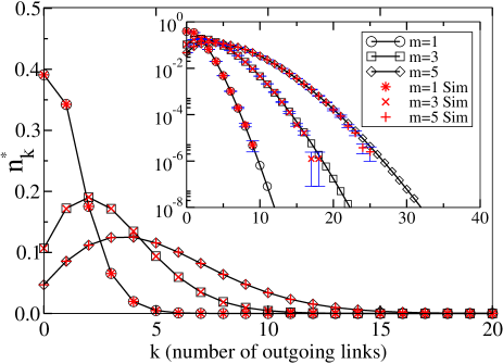
We also check our theoretical results by comparing them to results of Monte Carlo simulations. The growth scheme in the simulations is implemented as follows. We begin the simulation with $N_{0}\geq m$ nodes with $m$ incoming links each. At each time step, we add one new node. We pick a random existing node from the network, calculate the probability of attachment to that node, and generate a random number. If the random number is smaller than the attachment probability, we create a link between the new node and the randomly picked node. If not, we randomly pick another node from the network and repeat the process until the new node has $m$ links. (We do not pick the same node twice.) The direction of a new link is from the existing node to the new one. The simulation stops when the system size reaches $N_{\rm{max}}+N_{0}$ nodes. We take $N_{\rm{max}}=10^{6}$ and average the results over eight independent runs.

The results of the Monte Carlo simulations are also shown in Fig. 2. They are in excellent agreement with the theory. The deviations in the last three nonzero data points are consistent with the number of runs used for averaging.

In order to clarify the role of the low-degree preferential attachment, we provide some comparisons with similar models in the next section.

III The Role of the Low-degree Preferential Attachment and Relevance to Simple Food-Web Models

III.1 A growing network with degree-independent probability of attachment

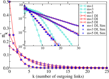
We first compare our model to an equivalent model with a degree-independent probability of attachment, $\Pi=1/N_{\rm T}$. In this case, $\Pi$ is the same for all nodes, however, it is time dependent. As we prove in Appendix C, a degree-independent $\Pi$ yields a network with an exponential outdegree distribution as seen in Fig. 3. This shows that the low-degree preferential attachment is responsible for the peaked form of $n_{k}^{*}$, and also for the faster decay in the tail.

III.2 The cascade model

Secondly, we test the effect of the low-degree preferential attachment in the cascade model CommunityFoodWebs ; Stouffer:2005 , which is a simple wiring-based food-web model. Although the cascade model has now mostly been replaced by improved variants like the niche model Martinez:2000 , it serves our purpose better, because it is quite simple and transparent. The cascade model builds a web using a few simple rules as follows. The species are numbered from 1 to $S$, where $S$ is the total number of species. Each species, $i$, is allowed to prey on a species $j$, where $i>j$, with a constant probability $x=d/S$, where $d\leq S$ is a constant. The species with no predators constitute the top species, and the species with no prey constitute the basal species  . The average number of prey (or predator) per species is equal to $(d/2)(1-1/S)\approx d/2$ for large $S$. Therefore, $d/2$ is analogous to $m$ in our growth model.

The calculation of the outdegree (predator) distribution of the webs produced by the cascade model is quite straightforward. First, we find the probability of finding a node, $i$, with $k$ outgoing links:

$${\cal P}_{i}^{\rm(out)}(k)={S-i\choose{k}}(1-x)^{S-i-k}x^{k}\qquad\textrm{with }k\leq S-i\;.$$ (13)

Then we obtain the outdegree distribution by summing ${\cal P}_{i}^{\rm(out)}(k)$ over $i$, and normalizing by $S$ :

$$p^{\rm(out)}(k)=\frac{1}{S}\sum_{i=1}^{S-k}{{\cal P}_{i}^{\rm(out)}(k)}\qquad\textrm{with }k<S\;.$$ (14)

The cascade model produces webs with identical in- and outdegree distributions. One can prove this by substituting ${\cal P}_{S-i+1}^{\rm(out)}(k)$ for ${\cal P}_{i}^{\rm(in)}(k)$ in $p^{\rm(in)}(k)=\sum_{i=k+1}^{S}{{\cal P}_{i}^{\rm(in)}(k)}/S$.

In order to see the effect of the low-degree preferential attachment, we modify the cascade model by changing the probability of attachment from a constant, $x=d/S$, to a decreasing function of the outdegree of the prey node, $x(k_{i})=d/[S(k_{i}+1)]$. (We note that for both original and modified cascade models, the probability of attachment does not depend on time, unlike in our proposed growth model.) Obviously, this modification does not conserve the expected total number of links. Nevertheless, it still demonstrates the effect of the low-degree preferential attachment in the cascade model. We also point out that the degree-dependent nature of this mechanism could cause different degree distributions in the cascade model, depending on the order in the wiring procedure. (See endnote  .) We leave extensive analysis to a further publication and give only these preliminary results here.

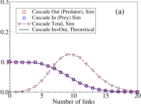
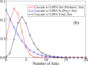
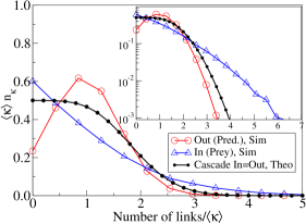
Fig. 4 shows the in- and outdegree distributions of the original and modified cascade models for $d=10$ and $S=10^{4}$. One can clearly discern two changes: the new in- and outdegree distributions are not identical, and they are also quite different than those of the original cascade model. The new outdegree distribution takes a similar form to the outdegree distribution in our model, $n_{k}^{*}$, in Eq. (11), and the new indegree distribution decays monotonically. For a better comparison, we also provide the scaled forms of these distributions in Fig. 5. The figure shows that the tail of the outdegree distribution is depressed, while the indegree distribution decays much slower than in the original cascade model. All the distributions decay faster than an exponential. The analytical forms of the distributions are left for further investigation.

One could also compare our results with the latest findings in food-web theory. According to Camacho et al. Camacho:2002A ; Camacho:2002B ; Stouffer:2005 , the predator and prey distributions for most empirical food webs obey universal functional forms. The universal form of the predator (outdegree) distribution is given by $p_{\rm pred}(k)=\gamma(k+1,z)/z$, where $\gamma(k,z)$ is the incomplete Gamma function and $z$ is the average connectivity, $2L/S$, with $L$ the total number of links in the web. This is a continuum approximation to Eq. (14) for $S\gg 1$ and $x\ll 1$. This form of the predator distribution suggested by Camacho et al. and the outdegree distribution of our model with low-degree preferential attachment, $n_{k}^{*}$, have some similarities, like the cut-off values and Gaussian-like, fast-decaying tails. A detailed assessment, however, requires further analysis, which we plan to publish elsewhere.

IV Summary

We have studied an attachment scheme for growing directed networks, in which a new node attaches to an existing node $i$ with a probability $\Pi(k_{i})\propto 1/k_{i}$, where $k_{i}$ is the number of outgoing links at $i$. The motivation behind this idea is the following. If the links supply resources to the nodes in the network, and if the nodes can get the resources only through other nodes, then a new node will prefer to attach to existing nodes with fewer outgoing links to minimize its competitors for resources. We obtained the steady-state outdegree distribution, $n_{k}^{*}$, which decays like $k\mu^{k}/\Gamma(k)$ for large $k$, where $\mu$ is a constant. In order to further understand the effects of the low-degree preferential attachment, we also studied an equivalent growth model with a constant probability of attachment, which yields an exponential outdegree distribution. We also implemented this mechanism in the cascade model. The low-degree preferential attachment caused a difference between in- and outdegree distributions in the modified cascade model (identical in the original model), as well as a significant depression in the tail of the outdegree distribution and a broadening of the tail of the indegree distribution. These results indicate that the main effect of the low-degree preferential attachment mechanism is the fast decay in the tails of the outdegree distributions.

Although we propose this scheme for growing transportation networks, we do not claim that this is the only factor that determines the topology of such networks. In fact, we do not believe that growing transportation networks can be realistically modeled using a semi-static growth scheme, in which only the new nodes are allowed to make new connections while the rest of the network is frozen. Our model also lacks some essential features like the conservation of energy or mass. As a result, the networks can grow indefinitely. Nevertheless, the scheme we propose could be taken as a first approximation to modeling a growing directed transportation network, in which the probability of attachment is a decreasing function of the number of outgoing links.

Appendix A Numerical Calculation of $z_{m}^{*}$

We use numerical methods to determine the values of $z_{m}^{*}$ for different $m$. Substituting Eq. (11) into Eq. (9), yields a self-consistent equation for $z_{m}^{*}$:

$$z_{m}^{*}=\sum_{k=0}^{\infty}\frac{(m/z_{m}^{*})^{k}\Gamma\big{(}1+m/z_{m}^{*}\big{)}}{\Gamma\big{(}k+2+m/z_{m}^{*}\big{)}}\;,$$ (15)

which can also be written as

$$z_{m}^{*}=\frac{\Phi(1,2+m/z_{m}^{*};m/z_{m}^{*})}{1+m/z_{m}^{*}}\;,$$ (16)

where $\Phi(1,2+m/z_{m}^{*};m/z_{m}^{*})$ is the degenerate hypergeometric function defined as $\Phi(a,b;z)=\sum_{n=0}^{\infty}{\frac{(a)_{n}z^{n}}{(b)_{n}n!}}$, where $(a)_{n}=a(a+1)(a+2)\ldots(a+n-1)$, with $(a)_{0}=1$ GradshteynHyper . The right-hand side of Eq. (16) is a smooth function of $z_{m}^{*}$. We obtain $z_{m}^{*}$ by solving Eq. (16) numerically for $m/z_{m}^{*}$ . For $m=1$, 3, and 5, we obtained $z_{m}^{*}=0.6419$, 0.3582 and 0.2467, respectively, which we used to plot the outdegree distribution, Eq. (11), in Fig. 2. The $m$-dependence of $z_{m}^{*}$ is shown in Fig. 6. As seen in the figure, $z_{m}^{*}$ is proportional to $m^{-1}$ for large $m$.

Appendix B Theoretical Calculation of the Scaling Function for the Growth Model with Low-degree Preferential Attachment

We scale $n_{k}^{*}$ by substituting $u=k/m$ and $p(u|m)=mn_{mu}$ in Eq. (8):

$$p(u|m)=\frac{(mu+1)}{z_{m}^{*}u[m/z_{m}^{*}+mu+1]}p(u-m^{-1}|m)\;.$$ (17)

By taking the logarithm of both sides, we obtain

$$\ln p(u|m)-\ln p(u-m^{-1}|m)=\ln\frac{1+1/mu}{1+z_{m}^{*}u+z_{m}^{*}/m}\;.$$ (18)

We convert the left-hand side to a derivative, and expand the right-hand side into a series assuming that $1/mu,z_{m}^{*}u$, and $z_{m}^{*}/m\rightarrow 0$ as $m\rightarrow\infty$:

$$\frac{1}{m}\frac{\partial}{\partial u}\ln p(u|m)=\frac{1}{mu}-\frac{z_{m}^{*}}{m}-z_{m}^{*}u\;.$$ (19)

This equation has a solution of the form

$$p(u|m)=Cu\exp(-z_{m}^{*}[u+mu^{2}/2])\;.$$ (20)

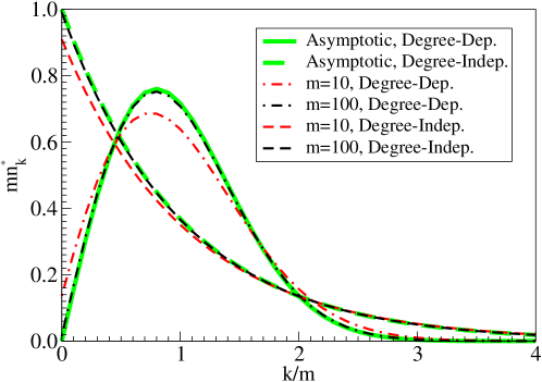
We require that $p(u|m)$ should be normalizable with $\langle u\rangle=1$ (recall that $\langle k\rangle=m$). In the limit $m\rightarrow\infty$, this requires that $z_{m}^{*}=a/m$, where $a$ is a constant. Using these conditions, we normalize $p(u|\infty)\equiv p(u)=Cu\exp(-au^{2}/2)$, obtaining $C=\pi/2$ and $z_{m}^{*}=\pi/2m$. The asymptotic function, $p(u)$, is given in Eq. (12) and shown in Fig. 7. The excellent agreement with $mn_{k}^{*}$ vs $k/m$ confirms our results.

This result also implies that the ratio of the standard deviation of $n_{k}^{*}$ to its mean, $\sigma/\langle k\rangle$, converges to a constant as $m$ increases. Therefore, $\sigma$ becomes proportional to $m$, since $\langle k\rangle$ is just $m$ . Fig. 6 shows that $\sigma/\langle k\rangle=\lambda+O(1/m)$ for large $m$. We obtain $\lambda=\lim_{m\rightarrow\infty}\sigma/\langle k\rangle$ using $p(u)$:

$$\lambda=\frac{\sqrt{\langle u^{2}\rangle-\langle u\rangle^{2}}}{\langle u\rangle}=(4/\pi-1)^{1/2}\approx 0.522\;.$$ (21)

Appendix C Theoretical Calculation of Outdegree Distribution for the Growth Model with Degree-Independent Probability of Attachment

We follow the same method we used to derive Eq. (11). Taking the probability of attachment independent of in- and outdegree, and also identical for all nodes, $\Pi=1/N_{\rm T}$, we obtain the rate equations for the outgoing links:

$$\frac{dN_{k}}{dt}=m\frac{N_{k-1}}{N_{\rm T}}-m\frac{N_{k}}{N_{\rm T}}\qquad\textrm{for }k>0\;.$$ (22)

Substituting $n_{k}N_{\rm T}$ for $N_{k}$, and using $dN_{\rm T}/dt=1$, yields equations for the density of nodes:

$$N_{\rm T}\frac{dn_{k}}{dt}=mn_{k-1}-(m+1)n_{k}\;.$$ (23)

In the steady state, we have

$$(m+1)n_{k}^{*}=mn_{k-1}^{*}\;.$$ (24)

The solution of this equation yields the steady-state outdegree distribution:

$$n_{k}^{*}=n_{0}^{*}c^{k}\;,$$ (25)

where $c=m/(1+m)$. Imposing the normalization condition, $\sum_{k}^{\infty}{n_{k}^{*}}=1$, we find, $n_{0}^{*}=1-c=1/(1+m)$.

We can also derive the scaling form of this distribution for comparison with the scaling form of Eq. (11) in Appendix B. Multiplying both sides of Eq. (25) by $m$, we get

$$mn_{k}^{*}=\left(\frac{m}{1+m}\right)^{k+1}=[(1+1/m)^{m}]^{-\frac{k+1}{m}}\;.$$ (26)

In the limit $m\rightarrow\infty$, this equation yields the scaling function

$$q(u)=mn_{k}^{*}=\exp(-u)\;,$$ (27)

with $u=k/m$. $q(u)$ is shown in Fig. 7.

As a result, the asymptotic ratio $\sigma/\langle k\rangle$ for the outdegree distribution is equal to unity, a characteristic of the exponential distribution, compared to $\lambda\approx 0.522$ in degree-dependent case.

References

- (1) A. L. Barabasi and R. Albert, Science 286, 509 (1999).
- (2) R. Albert and A. L. Barabasi, Rev. Mod. Phys. 74, 47 (2002).
- (3) S. N. Dorogovtsev, J. F. F. Mendes, and A. N. Samukhin, Phys. Rev. Lett. 85, 4633 (2000).
- (4) P. L. Krapivsky, S. Redner, and F. Leyvraz, Phys. Rev. Lett. 85, 4629 (2000).
- (5) P. L. Krapivsky and S. Redner, Phys. Rev. E 63, 066123 (2001).
- (6) S. N. Dorogovtsev, J. F. F. Mendes, and A. N. Samukhin, Phys. Rev. E 64, 025101(R) (2001).
- (7) G. J. Rodgers and K. Darby-Dowman, Eur. Phys. J. B 23, 267 (2001).
- (8) D. Garlaschelli, G. Caldarelli, and L. Pietronero, Nature (London) 423, 165 (2003).
- (9) J. R. Banavar, A. Maritan, and A. Rinaldo, Nature (London) 399, 130 (1999).
- (10) B. Drossel and A. J. McKane, in Handbook of Graphs and Networks: From the Genome to the Internet, edited by S. Bornholdt and H. G. Schuster (Wiley-VCH, Berlin, 2002).
- (11) J. A. Dunne, R. J. Williams, and N. D. Martinez, Proc. Natl. Acad. Sci. USA 99, 12917 (2002).
- (12) J. Montoya and R. Solé, Oikos 102, 614 (2003).
- (13) A. J. McKane, Eur. Phys. J. B 38, 287 (2004).
- (14) L. A. N. Amaral, A. Scala, M. Barthélémy, and H. E. Stanley, Proc. Natl. Acad. Sci. USA 97, 11149 (2000).
- (15) R. Albert, I. Albert, and G. L. Nakarado, Phys. Rev. E 69, 025103(R) (2004).
- (16) R. Guimera and L. A. N. Amaral, Eur. Phys. J. B 38, 381 (2004).
- (17) R. J. Williams and N. D. Martinez, Nature (London) 404, 180 (2000).
- (18) J. Camacho, R. Guimerà, and L. A. N. Amaral, Phys. Rev. E 65, 030901(R) (2002).
- (19) J. Camacho, R. Guimerà, and L. A. N. Amaral, Phys. Rev. Lett. 88, 228102 (2002).
- (20) D. Stouffer et al., Ecology 86, 1301 (2005).
- (21) J. E. Cohen, F. Briand, and C. E. Newman, Community Food Webs, Biomathematics Vol. 20 (Springer-Verlag, Berlin, 1990).
- (22) I. S. Gradshteyn and I. S. Ryzhik, Table of Integrals, Series and Products, Corrected and Enlarged Edition (Academic Press, New York, 1980), p. 1058, Formula No. 9.210-1.