Surface criticality in random field magnets

Abstract

The boundary-induced scaling of three-dimensional random field Ising magnets is investigated close to the bulk critical point by exact combinatorial optimization methods. We measure several exponents describing surface criticality: $\beta_{1}$ for the surface layer magnetization and the surface excess exponents for the magnetization and the specific heat, $\beta_{s}$ and $\alpha_{s}$. The latter ones are related to the bulk phase transition by the same scaling laws as in pure systems, but only with the same violation of hyperscaling exponent $\theta$ as in the bulk. The boundary disorders faster than the bulk, and the experimental and theoretical implications are discussed.

I Introduction

The presence of quenched randomness leads to many differences in the statistical behavior if compared to “pure systems”. This is true in many phenomena as transport properties in, for instance, superconductors, or in a rather wide range of cases in magnetism. Consider a domain wall in a magnet, which gets pinned due to impurities. The scenario may vary according to the symmetries of the system and to the character of the disorder, but is described, in most general terms, by an “energy landscape” which develops a rich structure due to the the presence of pinning defects generic .

The most usual and convenient example of such magnets is given by the Ising model -universality class. Disorder is normally introduced as frozen random bond” and “random field” impurities, which can change dramatically the nature of the phases of the model and the character of the phase transition. Strong enough bond disorder creates a spin glass -state, while the random fields couple directly to the order parameter, the magnetization.

The criticality in such models is usually studied by finite size scaling, to extract the thermodynamic behavior. However, real (experimental) systems are finite and have boundaries. These break the translational invariance and create differences in the critical behavior between the boundary region and the bulk. The related phenomenon is called “surface criticality”, and essential is that a whole set of new critical exponents arises, to describe the behavior of various quantities at and close to surfaces ptcp8 ; ptcp10 . Here, we investigate by scaling arguments and exact numerical methods this phenomenon in the case of the random field Ising model (RFIM), in three dimensions (3d). In this case, the RFIM has a bulk phase transition separating ferromagnetic and paramagnetic states.

The central question that we want to tackle is: how do disorder and the presence of boundaries combine, in a system where the critical bulk properties are already different from pure systems? Though disordered magnets have been investigated earlier for the case of weak bond-disorder selke ; pleimling , both spin-glasses - a possible future extension of our work - and the RFIM have not been studied heiko . One general problem of the 3d RFIM has been how to observe the critical behavior, and understanding the boundary critical behavior provides an independent, novel avenue for such purposes belanger ; antifm ; kleemann . Such experiments are done on a number of systems from diluted antiferromagnets in a field, belanger ; antifm , to binary liquids in porous media, dierker , and to relaxor ferroelectrics kleemann .

The particular characteristics of the RFIM is a complicated energy landscape, which manifests itself e.g. in the violation of the usual hyperscaling relation of thermodynamics, and in the existence of an associated violation exponent $\theta$ and several consequences thereof. This is analogous to, for instance, spin glasses, and furthermore for surface criticality presents the question how the broken translational invariance combines with the energy scaling. Our results imply that this can be understood by scalings that include both the bulk correlation length exponent $\nu$ and the bulk $\theta$ and novel surface exponents. Moreover, though the bulk RFIM 3d phase transition has been notoriously difficult experimentally, the boundary order parameter, say, should be quite sensitive to the control one (temperature, in experiments and disorder here) and promises thus to make the surface criticality experimentally observable.

In the next section we overview the theoretical picture, as applied to the RFIM. Section 3 presents the numerical results, where the emphasis is two-fold. We discuss the surface criticality on one hand, and on the other hand the decay of a surface field induced perturbation is analyzed, since it has characteristics peculiar to a disordered magnet, in contrast to pure systems. Finally, Section 4 finishes the paper with a discussion of the results and future prospects.

II Surface criticality

The RFIM Hamiltonian with a free surface $S$ reads

$$H_{RFIM}=-J\sum_{\langle i,j\rangle\notin S}\sigma_{i}\sigma_{j}-J_{1}\sum_{\langle i,j\rangle\in S}\sigma_{i}\sigma_{j}-\sum_{i}h_{i}\sigma_{i},$$ (1)

where $J$ is the bulk (nearest neighbour) interaction strength while $J_{1}$ describes the strength of the surface interaction, in general different from $J$. $\sigma_{i}$ take the values $\pm 1$. For simplicity, the random fields $h_{i}$ obey a Gaussian probability distribution $P(h_{i})=\frac{1}{\sqrt{2\pi}\Delta}\exp{\left[-\frac{1}{2}\left(\frac{h_{i}}{\Delta}\right)^{2}\right]}$, with a zero mean and standard deviation $\Delta$. One might have also external fields such as a bulk magnetic field $h$ and a surface magnetic field $h_{1}$ at $S$.

Being governed by a zero temperature fixed point, the phase transition of the 3d RFIM can also be studied at $T=0$, where it takes place at a critical $\Delta_{c}$. The transition is of second order though it also exhibits some first-order characteristics: the order parameter exponent $\beta$ is very close to zero middleton ; rieger ; hartmann_m . The surface criticality of the 3d RFIM is simplified by the fact that the lower critical dimension is two aizenman ; uusi , thus in the absence of a surface magnetic field $h_{1}$ just an ordinary transition can take place. The surface orders only because the bulk does so, and the transition point is the bulk critical point.

Even in this case, there is a wide variaty of surface quantities. Derivatives of the surface free energy $f_{s}$ (surface ground state energy at $T=0$) with respect to surface fields, as the surface magnetic field $h_{1}$, yield local quantities (e.g. the surface layer magnetization $m_{1}=-\partial f_{s}/\partial h_{1}$), while derivatives of $f_{s}$ with respect to bulk fields produce excess quantities, such as the excess magnetization $m_{s}=-\partial f_{s}/\partial h$, defined by

$$\frac{1}{V}\int d^{d}x\ m({\bf x})=m_{b}+\frac{S}{V}m_{s}+O(L^{-2}),$$ (2)

where $m(\bf x)$ is the (coarse grained) magnetization at ${\bf x}$ and $V\sim L^{d}$ and $S$ are the sample volume and its surface area, respectively. One also obtains mixed quantities by taking second or higher derivatives of $f_{s}$. We focus on the critical behavior of the local and the excess magnetization ($m_{1}$ and $m_{s}$) as well as the excess specific heat $C_{s}$.

The RFIM bulk critical exponents are related via the usual thermodynamic scaling relations, see Table 1. The hyperscaling relations, however, have the modified form

$$2-\alpha=\nu(d-\theta),$$ (3)

with the additional exponent $\theta$ braymoore . The usual way to relate the surface excess exponents to bulk exponents is to note that from the conventional hyperscaling (Eq. (3) with $\theta=0$) it follows that the singular part of the bulk free energy $f_{b}^{(sing)}$ scales with the correlation length $\xi$ as $f_{b}^{(sing)}\sim\xi^{-d}$. By making the analogous assumption for the surface free energy, $f_{s}^{(sing)}\sim\xi^{-(d-1)}$, one finds ptcp10

$$\alpha_{s}=\alpha+\nu,\quad\beta_{s}=\beta-\nu.$$ (4)

In the case of the RFIM the above becomes less clear: does the $\theta$-exponent get modifed? We assume that the exponent $\theta^{\prime}$ in $f_{s}^{(sing)}\sim\xi^{-(d-1-\theta^{\prime})}$ may in general be different from the bulk exponent $\theta$, and obtain

$$\alpha_{s} = \alpha+\nu-\nu(\theta-\theta^{\prime}),$$ (5)

$$\beta_{s} = \beta-\nu+\nu(\theta-\theta^{\prime}).$$ (6)

To derive Eq. (6), the scaling form $\frac{E_{s}^{(sing)}}{J}\sim t^{2-\alpha_{s}}\tilde{E}_{s}[h/Jt^{-(\gamma+\beta)}]$ is used for the singular part of the excess ground state energy density $E_{s}^{(sing)}$ (which takes the role of the excess free energy at $T=0$), with $t\equiv(\Delta-\Delta_{c})/J$, Eq. (5) and the Rushbrooke scaling law $\alpha+2\beta+\gamma=2$. $\gamma$ is the exponent describing the critical behavior of the bulk susceptibility. Scaling relations relating $\beta_{1}$ to other ’local’ surface exponents can also be derived, but it cannot be expressed in terms of bulk exponents alone.

Quantity	Definition	Exponent
excess magnetization	$m_{s}=-\frac{\partial f_{s}}{\partial h}$	$m_{s}\sim(-t)^{\beta_{s}}$
excess specific heat	$C_{s}=\frac{\partial^{2}f_{s}}{\partial\Delta\partial J}$	$C_{s}\sim|t|^{-\alpha_{s}}$
surface magnetization	$m_{1}=-\frac{\partial f_{s}}{\partial h_{1}}$	$m_{1}\sim(-t)^{\beta_{1}}$

Table 1: Surface quantities in terms of the surface free energy $f_{s}$, and the corresponding critical exponents ($t\equiv(\Delta-\Delta_{c})/J$). Note that $T=0$ so that one uses instead of a free energy the ground state energy.

III Numerical results

The exact ground state (GS) calculations are based on the equivalence of the $T=0$ RFIM with the maximum flow problem in a graph alavaptcp ; we use a polynomial push-relabel preflow-type algorithm goldberg ; seppala_vk . If not stated otherwise, we study cubic systems of size $L^{3}$, $L\leq 100$. Free boundary conditions are used in one direction (the free surface under study) while in the remaining ones periodic boundary conditions are imposed. The maximal statistical error in what follows is of the order of the symbol size used, so the error bars are omitted. Note that since in the present case only the ordinary transition is possible, the critical exponents should be independent of the surface interaction $J_{1}$. Complications arise, however, since in 2d the RFIM is effectively ferromagnetic below the break-up length scale $L_{b}$, which scales as $L_{b}\sim\exp{[A(J/\Delta)^{2}]}$ (see Fig. 1) seppala_Lb ; binder . This means that the surfaces have a tendency to be ordered “an sich”, and to see the true ordinary transition behavior, one needs $L>L_{b}$. Thus, we use substantially weakened surface interactions $J_{1}\ll J$ to circumvent this problem.

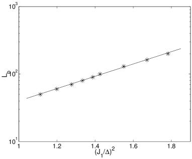
Figure 1: The break-up length scale $L_{b}$ of the 2d surface layer of the 3d RFIM with a strongly paramagnetic bulk, $J=0.05\Delta$, vs $(J_{1}/\Delta)^{2}$. $L_{b}$ is estimated by looking for a value of $J_{1}$ such that the surface will be totally ordered with probability $1/2$ while keeping $\Delta$ and $L$ fixed. The solid line corresponds to $A=2.1$.

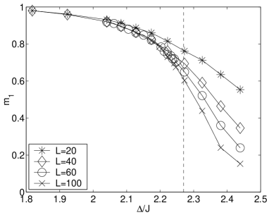
Figure 2: Mean absolute value of the surface layer magnetization $m_{1}$ as a function of $\Delta/J$ for various $L$, $J_{1}=J$. The dashed vertical line corresponds to the critical point of the infinite system, $\Delta/J=2.27$.

III.1 Surface layer magnetization

Fig. 2 shows an example of the magnetization $m_{1}$ of the surface layer close to $\Delta_{c}$, obtained directly from the spin structure of the GS. We assume the finite size scaling ansatz

$$m_{1}=L^{-\beta_{1}/\nu}\tilde{m}_{1}[(\Delta-\Delta_{c})L^{1/\nu}],$$ (7)

where $\tilde{m}_{1}$ is a scaling function. At the critical point $\Delta=\Delta_{c}$, Eq. (7) reduces to $m_{1}\sim L^{-\beta_{1}/\nu}$. Fig. 3 is a double logarithmic plot of $m_{1}$ versus $L$ at $\Delta_{c}/J=2.27$ for three $J_{1}$-values. All three are consistent with

$$\beta_{1}/\nu=0.17\pm 0.01.$$ (8)

Using the bulk value $\nu=1.37\pm 0.09$ middleton , one obtains

$$\beta_{1}=0.23\pm 0.03.$$ (9)

Fig. 4 depicts $m_{1}L^{\beta_{1}/\nu}$ versus $(\Delta-\Delta_{c})L^{1/\nu}$, and with $\beta_{1}/\nu=0.17$, $\nu=1.37$ and $\Delta_{c}/J=2.27$ one indeed obtains a decent data collapse. With $J_{1}\approx J$, however, plotting $m_{1}(\Delta_{c})$ versus $L$ produces a slightly different exponent, $\beta_{1}/\nu\approx 0.15$, and we could not get good data collapses, probably due to the fact that $L_{b}$ is large.

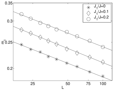
Figure 3: A log-log plot of the surface layer magnetization $m_{1}$ as a function of the system size $L$ at criticality, $\Delta/J=2.27$, for various $J_{1}/J\ll 1$. The solid lines depict fits, with $\beta_{1}/\nu=0.17\pm 0.01$ for all three cases shown

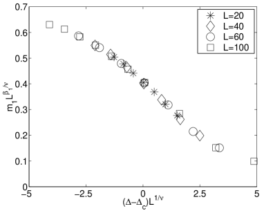
Figure 4: A scaling plot of the surface layer magnetization $m_{1}$ in the case $J_{1}=0$, $J=1$, using $\Delta_{c}=2.27$, $\nu=1.37$ and $\beta_{1}=0.23$.

III.2 Surface excess magnetization

For the surface excess magnetization $m_{s}$, we use the finite size scaling ansatz

$$m_{s}=L^{-\beta_{s}/\nu}\tilde{m}_{s}[(\Delta-\Delta_{c})L^{1/\nu}],$$ (10)

where $\tilde{m}_{s}$ is a scaling function. Since $\beta_{1}$ was found to be independent of $J_{1}/J$ as long as $J_{1}/J\ll 1$ (in the limit $L\rightarrow\infty$, the independence of the exponents on $J_{1}/J$ should hold for any $J_{1}/J$), one expects the same to apply for the other exponents as well and we thus consider here only the case $J_{1}/J=0.1$. At the critical point, $m_{s}$ grows almost linearly with $L$ (Fig. 5), with the exponent $-\beta_{s}/\nu=0.99\pm 0.02$. This yields, by again using $\nu=1.37\pm 0.09$,

$$\beta_{s}=-1.4\pm 0.1.$$ (11)

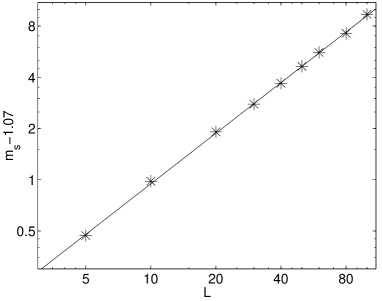
Figure 5: A log-log plot of the excess magnetization $m_{s}$ as a function of the system size $L$ for $\Delta/J=2.27$, $J_{1}/J=0.1$. A background term of magnitude 1.07 has been substracted from $m_{s}$ to see the power-law behavior. The solid line is a power-law fit, with $-\beta_{s}/\nu=0.99$.

III.3 Surface specific heat

In GS calculations, the specific heat is computed (recall $T=0$) by replacing the second derivative of the free energy $f$ with respect to the temperature by the second derivative of the GS energy density $E$ with respect to $\Delta$ or $J$ hartmann . $\partial E/\partial J$ is the the bond part of $E$, $E_{J}=L^{-d}\sum_{\langle i,j\rangle}\sigma_{i}\sigma_{j}$. The excess specific heat exponent $\alpha_{s}$ is estimated according to Ref. middleton (where the bulk one was considered). The singular part of the excess specific heat obeys

$$C_{s}^{(sing)}=L^{\alpha_{s}/\nu}\tilde{C}_{s}[(\Delta-\Delta_{c})L^{1/\nu}],$$ (12)

from which by integration it follows for the singular part of the excess bond energy at criticality,

$$E_{J,s}^{(sing)}(L,\Delta=\Delta_{c})=c_{1}+c_{2}L^{(\alpha_{s}-1)/\nu},$$ (13)

where $c_{1}$ and $c_{2}$ are constants. Fig. 6 is a plot of the excess bond energy, with $J_{1}/J=0.1$, at the bulk critical point. The fit using Eq. (13) results in $(\alpha_{s}-1)/\nu=0.22\pm 0.03$, corresponding to

$$\alpha_{s}=1.30\pm 0.05.$$ (14)

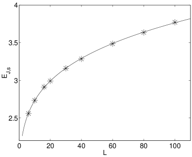
Figure 6: A plot of the absolute value of the excess bond energy $E_{J,s}$ as a function of $L$ for $\Delta/J=2.27$, $J_{1}/J=0.1$. The solid line corresponds to a fit of the form of Eq. (13), with $c_{1}=1.1292$, $c_{2}=0.9756$ and $(\alpha_{s}-1)/\nu=0.22.$

III.4 Magnetization decay close to the surface

Finally we discuss the behavior of the magnetization profiles $m(z)$ (i.e. magnetization as a function of the distance $z$ from the surface), in the case the spin orientation at the surface layer is fixed. This corresponds to applying a strong surface field $h_{1}$. These are of interest as they reflect spin-spin correlations close to the surface, as studied in Ref. parisisourlas in the slightly different context of comparing two replicas with opposite $h_{1}$. For the RFIM close to the infinite system bulk critical point, $m(z)$ is affected by the fact that for numerically feasible system sizes the bulk magnetization is close to unity and decreases very slowly with increasing system size (due to the small value of $\beta$) middleton . This is demonstrated in the inset of Fig. 7, where the distribution of bulk magnetization $m_{b}$ at the critical point can be seen to be strongly peaked around $m_{b}=\pm 1$.

One can now distinguish three scenarios from sample to sample: if $|m_{b}|\approx 1$ the applied strong surface field $h_{1}$ may have the same or opposite orientation, or finally the bulk magnetization $m_{b}$ may be close to zero. In the first case, the $h_{1}$ induced spin configuration will be close to the one in the absence of the field. In the second case, $h_{1}$ will either force $m_{b}$ to change sign altogether (producing again a flat profile with $m(z)\approx\pm 1$) or induce an interface between the two regions of opposite magnetization, as in Fig. 7. The third one has a small probability, and thus will not contribute much to the ensemble averaged magnetization profile. The average magnetization profile $\langle m(z)\rangle$ can then (for a finite system, at the infinite system critical point) be well approximated by writing

$$\langle m(z)\rangle\approx a+b\langle m_{if}(z)\rangle.$$ (15)

Here $a$ and $b$ are weight factors, here constant but in general function(s) of $L$, that tell the relative weight of samples where the magnetization changes inside due to the $h_{1}$.

$$\langle m_{if}(z)\rangle=\int dwdz_{0}P_{w}(w)P_{z_{0}}(z_{0})m(z,z_{0},w)$$ (16)

is the profile one would obtain by averaging only over “single sample” profiles $m(z,z_{0},w)$, corresponding to an interface of width $w$ and position $z_{0}$ (with probability distributions $P_{w}$ and $P_{z_{0}}$, respectively). A simplified model for $m(z,z_{0},w)$ is shown in Fig. 8.

From the exact ground state calculations, we identify the profiles corresponding to such interface configurations. This is done by demanding that such profiles have a region where $m(z)<-0.9$ (when $h_{1}\gg 0$). The interface width is defined as $w=z_{2}-z_{1}$, where $z_{1}$ and $z_{2}$ are the smallest $z$’s such that $m(z_{1})<0.9$ and $m(z_{2})<-0.9$, respectively. The interface position $z_{0}$ is then given by $z_{0}=(z_{1}+z_{2})/2$. By counting the fraction of such profiles, we can estimate $a$ and $b$ in Eq. (15). These have the approximate values of $0.39$ and $0.61$, respectively (for a system of size 40x40x80). By using Eqs. (15) and (16) with $m(z,z_{0},w)$ presented in Fig. 8, as well as the distributions $P_{w}$ and $P_{z_{0}}$ measured from the ground state calculations, one indeed obtains an average profile $\langle m(z)\rangle$ that is in reasonable agreement with the true one, see Fig. 9.

The average magnetization profile $\langle m(z)\rangle$ decays slowly with the distance $z$, not quite reaching zero at the opposite edge of the system in the case at hand. However, a typical value of $m(z)$ will be close to $\pm 1$ for all $z$, which persists for accessible system sizes due again to the small value of $\beta$. One may thus observe effects reminiscent of violation of self-averaging, and this would be true also if one would measure the averaged difference $\langle|m(z)-m_{GS}(z)|\rangle$ between the field-perturbed and GS configurations, and the higher moments thereof. These results illustrate simply how the quasi-ferromagnetic character of the 3d RFIM groundstate influences such perturbation studies, a consequence of the in practice limited system sizes one can access in simulations.

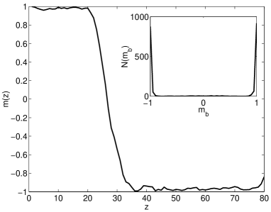
Figure 7: Main figure: A typical example of a magnetization profile, taken from a single sample, where due to a strong positive surface field $h_{1}$ at $z=0$ an interface has formed between two regions of opposite magnetization. Inset: Distribution of the bulk magnetization $m_{b}$ with periodic boundary conditions, 2000 samples. $\Delta/J=2.27$, system size 40x40x80.

Figure 8: A simple model for a single-sample magnetization profile $m(z,z_{0},w)$. The interface is characterized by the parameters position $z_{0}$ and width $w$.

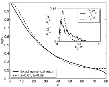
Figure 9: Main figure: A comparison between the numerical $\langle m(z)\rangle$ (solid line, averaged over $3000$ samples) and that obtained by using Eqs. (15) and (16) with $m(z,z_{0},w)$ as in Fig. 8 (dashed line). Inset: Distributions of the interface position $P_{z_{0}}(z_{0})$ (solid line) and width $P_{w}(w)$ (dashed line) obtained from the simulations. $\Delta/J=2.27$, system size 40x40x80.

IV Conclusions

In this work we have studied with combinatorial optimization and scaling arguments surface criticality in a random magnet, the 3d RFIM. The surface layer magnetization exponent $\beta_{1}$ is more than an order of magnitude larger than the extremely small bulk value middleton ; rieger ; hartmann_m . Experimentalists have reported much larger values for $\beta$ belanger ; antifm ; kleemann , which in fact are rather close to our estimate for $\beta_{1}$. An intriguing possibility in this respect is the direct observation of the surface order parameter in relaxor ferroelectrics via piezoelectric force microscopy kleemann2 .

The excess exponents $\alpha_{s}$ and $\beta_{s}$, when inserted into the scaling relations (5) and (6), both yield very small values for the correction term $\nu(\theta-\theta^{\prime})$, assuming $\alpha\approx 0$, $\beta\approx 0.02$ and $\nu\approx 1.37$ middleton . This suggests that in fact $\theta^{\prime}=\theta$, and the excess exponents are related to bulk exponents by the usual scaling laws valid for pure systems, Eq. (4). The numerically obtained description of the ordinary surface transition uses the bulk correlation length exponent as in pure systems. All this would merit further theoretical considerations and could also be checked in the four-dimensional RFIM 4drfim , whose phase diagram is also more complex due to the 3d surfaces which have independently phase transitions. The spin-spin correlations close to the surface and the magnetization profiles in the presence of boundary perturbations have been studied, similarly to the context of looking for self-averaging violations parisisourlas . It would be interesting to investigate this aspect in more detail, but in our numerics the most transparent features are due to the two-peaked magnetization distribution of the groundstates, without a perturbing field.

On a final note, the observations here concerning surface criticality in a disordered magnet - with a complicated energy landscape - extend directly for instance to spin glasses spinglasses and to a wide class of non-equilibrium systems (see fran , also for experimental suggestions). Two evident possibilities are looking for the same phenomenology in 3d Ising spin glasses, and in the 3d zero-temperature non-equilibrium RFIM. In the former case, the free surface of a system at $T>0$ is in analogy to the zero temperature 3d RFIM case inherently disordered (the 2d spin glass has a $T=0$ phase transition). In the second case, the situation is much more akin to the one at hand (fran ) and one should consider as the order parameter the remanent surface magnetization after a demagnetization procedure.

Acknowledgments A. Hartmann (Göttingen), D. Belanger (Santa Cruz) and W. Kleemann (Duisburg) are thanked for useful comments, and the Center of Excellence program of the Academy of Finland for financial support.

References

- (1) See for instance Spin Glasses and Random Fields, edited by A. P. Young (World Scientific, Singapore 1998).
- (2) K. Binder, in Phase Transitions and Critical Phenomena, eds. C. Domb and J. L. Lebowitz (Academic Press, London 1983), vol 8.
- (3) H. W. Diehl, in Phase Transitions and Critical Phenomena, eds. C. Domb and J. L. Lebowitz (Academic Press, London 1986), vol 10.
- (4) W. Selke, F. Szalma, P. Lajko and F. Igloi, J. Stat. Phys. 89, 1079 (1997).
- (5) M. Pleimling, J. Phys. A 37, R79 (2004).
- (6) An exception is the random transverse Ising chain, in which the influence of open boundaries has been studied. See e.g. F. Igloi and H. Rieger, Phys. Rev. B 57, 11404 (1998).
- (7) D. P. Belanger, in generic .
- (8) F. Ye et al., Phys. Rev. Lett. 89, 157202 (2002).
- (9) T. Granzow, Th. Woike, M. Wöhlecke, M. Imlau, and W. Kleemann, Phys. Rev. Lett. 92, 065701 (2004).
- (10) S. B. Dierker and P. Wiltzius, Phys. Rev. Lett. 58, 1865 (1987).
- (11) M. Aizenman and J. Wehr, Phys. Rev. Lett. 62, 2503 (1989).
- (12) G. Tarjus and M. Tissier, Phys. Rev. Lett. 93, 267008 (2004).
- (13) A. A. Middleton and D. S. Fisher, Phys. Rev. B 65, 134411 (2002).
- (14) H. Rieger, Phys. Rev. B 52, 6659 (1995).
- (15) A. K. Hartmann and U. Nowak, Eur. Phys. J. B 7, 105 (1999).
- (16) A. J. Bray and M. A. Moore, J. Phys. C 18, L927 (1985).
- (17) M. Alava, P. Duxbury, C. Moukarzel, and H. Rieger, in Phase Transitions and Critical Phenomena, eds. C. Domb and J. L. Lebowitz (Academic Press, San Diego 2001), vol 18.
- (18) A. V. Goldberg and R. E. Tarjan, J. Assoc. Comput. Mach. 35, 921 (1988).
- (19) E. Seppälä, PhD thesis, Dissertation 112 (2001), Laboratory of Physics, Helsinki University of Technology.
- (20) E. T. Seppälä, V. Petäjä, and M. J. Alava, Phys. Rev. E 58, R5217 (1998); E. T. Seppälä and M. J. Alava, Phys. Rev. E 63, 036126 (2001).
- (21) K. Binder, Z. Phys. B: Condens. Matter 50, 343 (1983).
- (22) A. K. Hartmann and A. P. Young, Phys. Rev. B 64, 214419 (2001).
- (23) W. Kleemann, J. Dec, P. Lehnen, R. Blinc, B. Zalar, and R. Pankrath, Europhys. Lett.. 57, 14 (2002).
- (24) G. Parisi and N. Sourlas, Phys. Rev. Lett. 89, 257204 (2002).
- (25) A. A. Middleton, cond-mat/0208182; note that for binary the transition is first-order: M.R. Swift et al., Europhys. Lett. 38, 273 (1997).
- (26) A. K. Hartmann and A.P. Young, Phys. Rev. B 64, 180404 (2001); A. C. Carter, A. J. Bray, and M. A. Moore, Phys. Rev. Lett. 88, 077201 (2002); J.-P. Bouchaud, F. Krzakala, and O. C. Martin, Phys. Rev. B 68, 224404 (2003).
- (27) F. Colaiori et al., Phys. Rev. Lett. 92, 257203 (2004).