Abstract

We study the response of a large array of coupled nonlinear oscillators to parametric excitation, motivated by the growing interest in the nonlinear dynamics of microelectromechanical and nanoelectromechanical systems (MEMS and NEMS). Using a multiscale analysis, we derive an amplitude equation that captures the slow dynamics of the coupled oscillators just above the onset of parametric oscillations. The amplitude equation that we derive here from first principles contains uncommon nonlinear gradient terms which yield a unique wave-number dependent bifurcation similar in character to the behavior known to exist in fluids undergoing the Faraday wave instability. We suggest a number of experiments with nanomechanical or micromechanical resonators to test the predictions of our theory, in particular the strong hysteretic dependence on the drive amplitude.

Tel-Aviv University

Raymond and Beverly Sackler

Faculty of Exact Sciences

School of Physics and Astronomy

Response of Discrete Nonlinear

Systems With Many Degrees of Freedom

Thesis submitted by Yaron Bromberg in partial fulfillment of the requirements for a M.Sc. degree in physics.

This work was carried out under the supervision of

Dr. Ron Lifshitz.

October 2004

revised on October 2005

Introduction

In the last decade we have witnessed exciting technological advances in the fabrication and control of microelectromechanical and nanoelectromechanical systems (MEMS and NEMS). Such systems are being developed for a host of nanotechnological applications, as well as for basic research in the mesoscopic physics of phonons, and the general study of the behavior of mechanical degrees of freedom at the interface between the quantum and the classical worlds [1, 2, 3]. Surprisingly, NEMS have also opened up a new experimental window into the study of the nonlinear dynamics of discrete systems with many degrees of freedom. A combination of three properties of NEMS resonators has led to this unique experimental opportunity. First and most important is the experimental observation that micro- and nanomechanical resonators tend to behave nonlinearly at very modest amplitudes. This nonlinear behavior has not only been observed experimentally [4, 5, 6, 7, 8, 9, 10, 11], but has already been exploited to achieve mechanical signal amplification and mechanical noise squeezing [12, 13] in single resonators. Second is the fact that at their dimensions, the normal frequencies of nanomechanical resonators are extremely high—recently exceeding the 1GHz mark [14]—facilitating the design of ultra-fast mechanical devices, and making the waiting times for unwanted transients bearable on experimental time scales. Third is the technological ability to fabricate large arrays of MEMS and NEMS resonators whose collective response might be useful for signal enhancement and noise reduction, as well as for sophisticated mechanical signal processing applications. Such arrays have already exhibited interesting nonlinear dynamics ranging from the formation of extended patterns [15]—as one commonly observes in analogous continuous systems such as Faraday waves—to that of intrinsically localized modes [16]. Thus, nanomechanical resonator arrays are perfect for testing dynamical theories of discrete nonlinear systems with many degrees of freedom. At the same time, the theoretical understanding of such systems may prove useful for future nanotechnological applications.

This work is motivated by a recent experiment of Buks and Roukes [15], who succeeded in fabricating, exciting, and measuring the response to parametric excitation of an array of 67 micromechanical resonating gold beams. Lifshitz and Cross [17] described the response of the beams with a set of coupled nonlinear differential equations (2.4). They used secular perturbation theory to convert these equations into a set of coupled nonlinear algebraic equations for the normal mode amplitudes of the system, enabling them to obtain exact results for small arrays but only a qualitative understanding of the dynamics of large arrays. In order to obtain analytical results for large arrays we study here the same system of equations, approaching it from the continuous limit of infinitely-many degrees of freedom. Our central result is a scaled amplitude equation (5.20), governed by a single control parameter, that captures the slow dynamics of the coupled oscillators just above the onset of parametric oscillations. This amplitude equation includes uncommon nonlinear gradient terms and exhibits a unique wave-number dependent bifurcation that can be traced back to the parameters of the equations of motion of the system (2.4). We confirm this behavior numerically and make suggestions for testing it experimentally.

This thesis is organized as follows. Chapters 1-3 serve as a brief background, summarizing the results of Buks and Roukes (chapter 1) and Lifshitz and Cross (chapters 2,3) that are essential for the understanding of the work presented in the following chapters. In chapter 4 we present a detailed description of our derivation of the amplitude equations describing the response of large arrays. A reduction to a single amplitude equation just above the onset of oscillations is preformed in chapter 5. Single mode solutions of the amplitude equation are discussed in chapter 6, and experimental schemes for obtaining such solutions and their unique properties are suggested and demonstrated numerically in chapter 7.

Chapter 1 Experimental Motivation

This work is motivated by a recent experiment of Buks and Roukes  [15, henceforth BR] who constructed an array of micromechanical resonating beams forming a diffraction grating. Fig. 1.1 shows a micrograph of 67 gold beams that BR fabricated on top of a silicon nitride membrane. Each beam was $270\times 1\times 0.25$ $\mu m$ in size, and the distance between two neighboring beams was $4\mu m$. The membrane was then removed, leaving only the ends of the beams connected to the silicon surface. Electrostatic forces between the beams were applied by connecting them alternately to two base electrodes. Such forces induce tunable coupling between the beams, and thus a collective spectrum of vibrational modes could be obtained. By introducing an ac component to the electrostatic forces, these modes can be parametrically excited. Optical diffraction was used to study the response of the array as a function of the driving frequency and the dc component of the electrostatic forces, $V_{dc}$. BR excited the array near its second instability tongue, i.e. the driving frequency lied within the band of normal frequencies (see chapter 2).

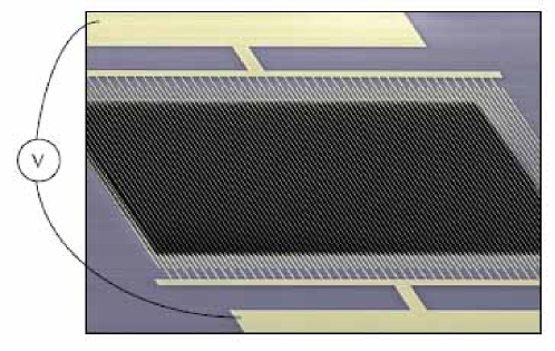
Figure 1.1: A side view micrograph of the array constructed by Buks and Roukes. The purple background is the silicon surface, from which a rectangular piece was etched away (black rectangular), leaving the fabricated gold beams connected to the silicon surface from both edges. A potential difference $V$ is applied between the two base electrodes.

Before applying the electrostatic forces, the characteristics of each beam separately were measured. The averaged fundamental frequency was $179.3$ kHz, with a standard deviation of $0.53$ kHz, and the quality factors $Q$ ranged from $2,000$ to $10,000$. No correlations were found between the location of the beams in the array and their specific properties. Therefore in the following model (chapter 2) the beams are regarded as identical. Once the electrostatic forces were applied, the quality factor values severely decreased as $V_{dc}$ was increased. This suggests that the dissipation of the system is mainly due to induced currents between the beams.

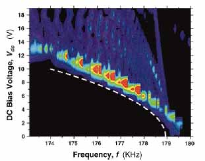
Figure 1.2: A color map showing relative intensities of the diffracted light from the array, as a function of the voltage $V_{dc}$ and the driving frequency $f$ taken from [15]. The dashed white line shows a fit to the measured lower bound frequency obtained from a simple linear theory. For $V_{dc}\approx 14V$ the array responded at frequencies beyond the expected upper bound frequency $f_{b}\approx 179.3kHz$.

Fig. 1.2 shows the measured collective response of the array as a function of the dc component of the electrostatic forces and the driving frequency. For each value of $V_{dc}$ the amplitude of the ac component was set to $50$ mV and the frequency was gradually increased. The band of frequencies the array responded to became wider as $V_{dc}$ was increased. This can be understood already at the linear analysis level, it is a direct consequence of the formation of the band of collective modes. The larger the dc component is, the wider is the band. The upper bound of the band however strongly depends on $V_{dc}$, while the linear analysis predicts it to be simply the fundamental frequency of an individual beam $\omega_{b}/2\pi\approx 179.3$ kHz. Moreover, for certain values of the dc component the array responded to frequencies beyond this upper bound frequency. It is also evident that as the driving frequency was swept up, the response showed a small number of wide peaks, much wider than the 67 resonance peaks that a linear theory predicts. These features were qualitatively explained by Lifshitz and Cross [17] by taking into account the nonlinearities of the array.

Chapter 2 Model and Equations of Motion

Lifshitz and Cross [17, henceforth LC] showed that the nontrivial response of the array is a direct consequence of the nonlinear character of the beams. They derived a set of equations of motion, introducing only the essential terms for capturing the nonlinear features obtained by BR. We shall briefly discuss some of their main guidelines for deriving the equations of motion.

The normal frequencies of the individual beams were found to be well separated. Thus for moderate driving each beam is strictly vibrating in its fundamental frequency $\omega_{b}$. Assuming the beams are restricted to in-plane vibrations only, each beam can be described by a single degree of freedom $u_{n}$, its displacement from equilibrium.

For simplicity, the attractive forces due to the applied electrostatic potential between the beams are approximated by nearest neighbor interactions

$$F_{electric}^{(n)}=-\frac{1}{2}m\omega_{b}^{2}\Delta^{2}[1+H\cos(2\omega_{p}t)](u_{n+1}-2u_{n}+u_{n-1}).$$ (2.1)

$\Delta^{2}$ and $\Delta^{2}H$ are the dc and ac components of the electrostatic forces respectively, where the prefactor $m\omega_{b}^{2}/2$ is inserted for convenience. The parametric excitation introduced into the system by the ac component, is an instability of the system that occurs for driving frequencies $2\omega_{p}$ close to one of the special values $2\omega_{0}/n$ [18], where $\omega_{0}$ is one of the normal frequencies of the array and $n$ is an integer that labels the so-called instability tongues of the system. In the BR experiment, the system was excited in its second instability tongue, i.e. $n=2\;,\omega_{p}\approx\omega_{0}/2$. Since the response at the second tongue was found to be quite similar to the response at the first tongue, the calculations preformed by LC were done for the first instability tongue. In the current work we proceed with concentrating on the first tongue only, and thus we always take $\omega_{p}$ itself to lie within the normal frequency band.

The restoring forces of the beams are due to their elasticity. Measurements done on individual beams indicate that the linear restoring force is supplemented with a cubic term of the displacement acting to stiffen the beam. Neglecting higher order nonlinear corrections the elastic force can therefore be written as

$$F_{elastic}^{(n)}=-m\omega_{b}^{2}\left(u_{n}+\alpha u_{n}^{3}\right),$$ (2.2)

with $\alpha>0$. Motivated by the observations of BR regarding the quality factors (see chapter 1) LC assumed that the dissipation of the system is mainly due to the electrostatic interaction, which induces currents through the beams. Therefore the dissipation should depend on the difference variable $u_{n}-u_{n-1}$, describing the relative displacements of a pair of neighboring beams. LC showed that a nonlinear dissipation term must also be introduced in order to obtain bounded response for driving frequency sweeps. Thus the dissipation terms were taken to be

$$F_{diss}^{(n)} =\frac{1}{2}m\omega_{b}\Gamma(\dot{u}_{n+1}-2\dot{u}_{n}+\dot{u}_{n-1})$$ (2.3)

$$+\ \frac{1}{2}m\omega_{b}\alpha\eta[(u_{n+1}-u_{n})^{2}(\dot{u}_{n+1}-\dot{u}_{n})-(u_{n}-u_{n-1})^{2}(\dot{u}_{n}-\dot{u}_{n-1})].$$

The dissipation of the system is assumed to be weak, which makes it possible to excite the beams with relatively small driving amplitudes. In such case the response of the beams is moderate, justifying the description of the system with nonlinearities up to cubic terms only. The weak dissipation can be parameterized by introducing a small expansion parameter $\epsilon\ll 1$, physically defined by the linear dissipation coefficient $\Gamma\equiv\epsilon\gamma$, with $\gamma$ of order one. The driving amplitude is then expressed by $\Delta^{2}H=\epsilon h$, with $h$ of order one. The weakly nonlinear regime is studied by expanding the displacements $u_{n}$ in powers of $\epsilon$. Taking the leading term to be of the order $\epsilon^{1/2}$ ensures that all the corrections, to a simple set of equations describing $N$ coupled harmonic oscillators, enter the equations at the same order of $\epsilon^{3/2}$.

Introducing the scaled variables $t\rightarrow t/\omega_{b}$ and $u_{n}\rightarrow u_{n}/\sqrt{\alpha}$, LC eventually obtained the following set of dimensionless equations

$$\ddot{u}_{n} + u_{n}+u_{n}^{3}+\frac{1}{2}\bigl{[}\Delta^{2}+\epsilon h\cos(2\omega_{p}t)\bigr{]}(u_{n+1}-2u_{n}+u_{n-1})$$ (2.4)

$$- \frac{1}{2}\epsilon\gamma(\dot{u}_{n+1}-2\dot{u}_{n}+\dot{u}_{n-1})$$

$$- \frac{1}{2}\eta\bigl{[}(u_{n+1}-u_{n})^{2}(\dot{u}_{n+1}-\dot{u}_{n})-(u_{n}-u_{n-1})^{2}(\dot{u}_{n}-\dot{u}_{n-1})\bigr{]}=0.$$

The boundary conditions are set according to the experiment of BR, who had two additional fixed beams at both ends of the array, thus $u_{0}=u_{N+1}=0$.

Chapter 3 Normal Modes and Linear Stability Analysis

We first expand the response of the beams into $N$ standing waves,

$$u_{n}=\sum_{m=1}^{N}\Phi_{m}(t)\sin(q_{m}n),\quad{\rm with}\quad q_{m}=\frac{m\pi}{N+1},\quad m=1\ldots N.$$ (3.1)

Substituting (3.1) into the equations of motion (2.4) yields $N$ nonlinear ODEs for the amplitudes of the waves,

$$\ddot{\Phi}_{m}+\omega_{m}^{2}\Phi_{m}+\epsilon 2\sin^{2}(q_{m}/2)\left[\gamma\dot{\Phi}_{m}-h\cos(2\omega_{p}t)\Phi_{m}\right]+N.L.=0,$$ (3.2)

where $N.L.$ stands for nonlinear terms that couple the $N$ linear Mathieu [19] equations, and $\omega_{m}$ is given by the dispersion relation

$$\omega^{2}_{m}=1-2\Delta^{2}\sin^{2}(q_{m}/2).$$ (3.3)

One can easily verify that the zero-displacement state, $u_{n}=0$ for all $n$, is always a solution of the equations of motion (2.4), though it is not always a stable one. To study the transition to oscillating solutions, we first linearize the equations of motion about the zero-displacement state, and introduce a new time scale $T=\epsilon t$ upon which the growth of small perturbations will occur. $T$ and $t$ are regarded as independent variables, following the multiple scales procedure [18], as we expand the response in orders of $\epsilon$,

$$\Phi_{m}(t,T)=\epsilon^{1/2}\Phi_{m_{0}}(t,T)+\epsilon^{3/2}\Phi_{m_{1}}(t,T)+O(\epsilon^{5/2}),$$ (3.4)

and express the time derivatives in terms of both $t$ and $T$,

$$\partial_{t}\rightarrow\partial_{t}+\epsilon\partial_{T}\quad{\rm and}\quad\partial^{2}_{tt}\rightarrow\partial^{2}_{tt}+2\epsilon\partial^{2}_{tT}+O(\epsilon^{2}).$$ (3.5)

Substituting (3.5) into the linear part of Eq. (3.2) and collecting terms of same order $\epsilon$ we obtain for the $\epsilon^{1/2}$ order terms

$$\left(\partial^{2}_{tt}+\omega_{m}^{2}\right)\Phi_{m_{0}}=0,$$ (3.6a)

and for the $$\epsilon^{3/2}$$ order terms

$$\left(\partial^{2}_{tt}+\omega_{m}^{2}\right)\Phi_{m_{1}}=\left(-2\partial^{2}_{tT}-2\gamma\sin^{2}\left(q_{m}/2\right)\partial_{t}+h\sin^{2}\left(q_{m}/2\right)(e^{i2\omega_{p}t}+e^{-i2\omega_{p}t})\right)\Phi_{m_{0}}.$$ (3.6b)

It is convenient to write the solution of Eq. (3.6a) in the following form

$$\Phi_{m_{0}}=A(T)e^{i\omega_{m}t}+c.c.\,,$$ (3.7)

where $A(T)$ is a complex amplitude which can slowly change over long time scales. Substituting into Eq. (3.6b) we obtain

$$\left(\partial^{2}_{tt}+\omega_{m}^{2}\right)\Phi_{m_{1}}= - \left(2i\omega_{m}\frac{dA_{m}}{dT}+2i\omega_{m}\gamma\sin^{2}\left(q_{m}/2\right)A_{m}\right)e^{i\omega_{m}t}$$

$$+ h\sin^{2}\left(q_{m}/2\right)A_{m}e^{i(2\omega_{p}+\omega_{m})t}+h\sin^{2}\left(q_{m}/2\right)A_{m}^{*}e^{i(2\omega_{p}-\omega_{m})t}+c.c.$$

The terms on the right hand side of Eq. (3) proportional to $e^{i\omega_{m}t}$ (called secular terms) excite the equation for $\Phi_{m_{1}}$ in its resonant frequency. In order to prevent the perturbative term $\Phi_{m_{1}}$ from diverging, we must account for a solvability condition, demanding that the sum of all the secular terms vanishes. For large frequency detunings $\omega_{p}-\omega_{m}\gg\epsilon$, only the first two terms of the left hand side of Eq. (3) must vanish and the solvability condition calls

$$\frac{dA_{m}}{dT}=-\gamma\sin^{2}(q_{m}/2)A_{m},$$ (3.9)

yielding a slow exponential decay of $A_{m}$ and thus no excitation of the $m^{th}$ mode. On the other hand for frequency detunings of order $\epsilon$ the fourth term of the right hand side of Eq.  (3) is also secular. We introduce a detuning parameter $\omega_{p}=\omega_{m}+\frac{1}{2}\epsilon\Omega_{m}$, and the solvability condition yields

$$-\left(2i\omega_{m}\frac{dA_{m}}{dT}+2i\omega_{m}\gamma\sin^{2}(q_{m}/2)A_{m}\right)+h\sin^{2}(q_{m}/2)A_{m}^{*}e^{i\Omega_{m}T}=0.$$ (3.10)

Trying a solution of the form $A_{m}(T)=a_{m}e^{\sigma_{m}T}e^{i\frac{\Omega_{m}}{2}T}$, with $\sigma_{m}\in\mathbb{R}$ yields

$$-2i\omega_{m}\sigma_{m}a_{m}+\omega_{m}\Omega_{m}a_{m}-2i\omega_{m}\gamma\sin^{2}(q_{m}/2)a_{m}+h\sin^{2}(q_{m}/2)a_{m}^{*}=0\quad\Rightarrow$$

$$(\omega_{m}\Omega_{m})^{2}+\left(2\omega_{m}\gamma\sin^{2}(q_{m}/2)+2\omega_{m}\sigma_{m}\right)^{2}=h^{2}\sin^{4}(q_{m}/2)\quad\Rightarrow$$

$$\sigma_{m}=-\gamma\sin^{2}(q_{m}/2)\pm\sqrt{(h\sin^{2}(q_{m}/2)/2\omega_{m})^{2}-(\Omega_{m}/2)^{2}}.$$ (3.11)

If the linear growth rate $\sigma_{m}>0$ the solution will grow, thus the critical driving amplitude $h_{m}(\omega_{p})$ is the one for which the growth rate $\sigma_{m}$ vanishes, explicitly,

$$h_{m}(\omega_{p})=2\omega_{m}\gamma\sqrt{1+\left(\frac{\Omega_{m}}{2\gamma\sin^{2}(q_{m}/2)}\right)^{2}}=2\omega_{m}\gamma\sqrt{1+\left(\frac{\omega_{p}-\omega_{m}}{\epsilon\gamma\sin^{2}(q_{m}/2)}\right)^{2}}.$$ (3.12)

$h_{m}(\omega_{p})$ is the driving amplitude required to excite the $m^{th}$ normal mode, from zero displacement into parametric oscillations with frequency $\omega_{p}$. Note that it has the familiar form of a first instability tongue [19], modified by the dispersive correction $\sin^{2}(q_{m}/2)$.

3.1 The Case of Distinct Normal Frequencies - A Single Mode Response

If the spacing between the normal frequencies $\delta\omega_{m}=\omega_{m}-\omega_{m-1}$ is much greater than $\epsilon$ one should expect the system to respond like a single degree of freedom. Only the mode for which $\omega_{p}$ is close to its normal frequency is excited. Fig. 3.1 $(A)$ shows five $h_{m}(\omega_{p})$ curves in the $(h,\omega_{p})$ plane which mark the onset of standing waves with a wave number $q_{m}$ for an array of 5 resonating beams. The curves do not overlap, indicating that in this array for moderate drives only single modes are excited.

In order to calculate the steady state response, a single mode solution should be substituted into the equations of motion (2.4)

$$u_{n}=\Phi_{m}(t)\sin(q_{m}n).$$ (3.13)

By taking into account the nonlinear terms neglected up to this point, the saturation of $A_{m}$ can be calculated. LC performed such a calculation and obtained the steady state of the single mode solution

$$u_{n} = \epsilon^{1/2}2|a_{m}|\cos(\omega_{p}t-\varphi)\sin(q_{m}n),\;{\rm with}$$

$$h^{2} = \frac{1}{\sin^{4}(q_{m}/2)}\left(\frac{9}{4}|a_{m}|^{2}-\omega_{m}\Omega_{m}\right)^{2}+\left(2\omega_{m}\gamma+6\omega_{m}\eta\sin^{2}(q_{m}/2)|a_{m}|^{2}\right)^{2},\;{\rm and}$$

$$\varphi = \frac{1}{2}\arctan\left(\frac{2\sin^{2}(q_{m}/2)\gamma+6\sin^{4}(q_{m}/2)\eta|a_{m}|^{2}}{\frac{9}{4}|a_{m}|^{2}-\omega_{m}\Omega_{m}}\omega_{m}\right).$$

In Fig. 3.1 $(B)$ and $(C)$ the response of the excited $m^{th}$ mode $|a_{m}|^{2}$ is plotted as a function of the amplitude $h$ for two values of the frequency detuning $\Omega_{m}$. Solid curves indicate stable solutions and dashed curves unstable solutions. The nature of the response changes significantly as the detuning is set above a critical value of $\Omega_{c}=16\sin^{6}(q_{m}/2)\omega_{m}\gamma\eta/3$. For $\Omega_{m}<\Omega_{c}$ the amplitude of the oscillating solution grows continuously for $h$ above threshold $h>h_{m}(\omega_{p})$ and is stable. This is known as a supercritical Hopf bifurcation [20]. On the other hand, a subcritical Hopf bifurcation is obtained for $\Omega_{m}>\Omega_{c}$. An unstable solution grows below threshold, until it reaches the so-called saddle-node point, where the curve of $|a_{m}|^{2}$ as a function of $h$ bends around (a turning point), and the solution becomes stable and an increasing function of $h$. The stability of the steady state solution is determined by linearizing the solutions (3.14) about a small perturbation with the same spatial dependence $\sin(q_{m}n)$ (see section 6.3 bellow). Whether these perturbations decay or grow determines the stability of the solution. The stability can alternatively be deduced from a corollary of the factorization theorem [21], which states that the stability of the solutions switches either at turning points or at points at which two solutions intersect. In both approaches only instabilities towards the growth of perturbations with the same wave number $q_{m}$ are examined, thus such a stability analysis is valid only for cases of sufficiently separated normal frequencies.

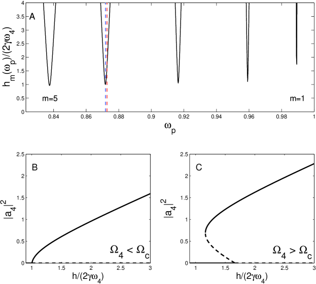
Figure 3.1: (A) The five $h_{m}(\omega_{p})$ curves of an array of 5 beams in the $(h,\omega_{p})$ plane are shown. Inside the region bounded by the $m^{th}$ curve the zero displacement state is unstable towards the growth of the $m^{th}$ mode. The dashed vertical lines mark two excitations of the array with frequency detunings of $\Omega_{4}=0.1$ (blue line) and $\Omega_{4}=2$ (red line). The critical detuning is $\Omega_{c}=0.196$. (B) For $\Omega_{4}<\Omega_{c}$ a supercritical bifurcation is obtained , (C) while $\Omega_{4}>\Omega_{c}$ yields a subcritical bifurcation. The parameters used are $\Delta=0.4,\;\eta=0.1$ and $\epsilon\gamma=0.001$.

3.2 The Case Overlapping Stability Curves

If $N$ is sufficiently large such that $\delta\omega_{m}\simeq\frac{\partial\omega_{m}}{\partial q_{m}}\frac{\pi}{N}\sim\frac{\Delta^{2}}{N}\sim\epsilon$, several modes can be excited simultaneously for moderate driving amplitudes $h\sim O(1)$. This situation is illustrated for $N=100$ oscillators in Fig. 3.2 which shows in (A) a set of overlapping instability tongues $h_{m}(\omega_{p})$ for $64<m<81$ plotted as a function of $\omega_{p}$, and in (B) the values of $h_{m}(\omega_{p})$ as a function of mode number $m$ for a particular value of $\omega_{p}=\omega_{73}$ (dashed line in (A)), outlining the neutral stability curve below which the zero-displacement state is stable.

In the limit $N\to\infty$ of very large arrays, the frequency spectrum becomes essentially continuous and so does the neutral stability curve of Fig. 3.2 (B). The first mode $q_{c}$ to emerge when increasing the driving amplitude from zero will then be the mode which minimizes the continuous $h_{m}(\omega_{p})$ curve, occurring at a critical driving amplitude $h_{c}$. For a moderate-size system, with a discrete frequency spectrum, the first excited mode $q_{m}$ will be the one whose critical driving amplitude $h_{m}(\omega_{p})$ is closest to $h_{c}$. By further increasing the driving amplitude, the zero-displacement state becomes unstable to a band of wave numbers bounded by the neutral stability curve, as indicated by the horizontal line in Fig. 3.2 (B). Once the excited modes start saturating into standing waves they interact with each other through the nonlinear terms, potentially yielding complicated dynamical behavior, as observed by LC [17] in the exact solutions obtained using secular perturbation theory. The exact solutions however could only be obtained for small arrays, enabling only a qualitative understanding of the dynamics of large arrays.

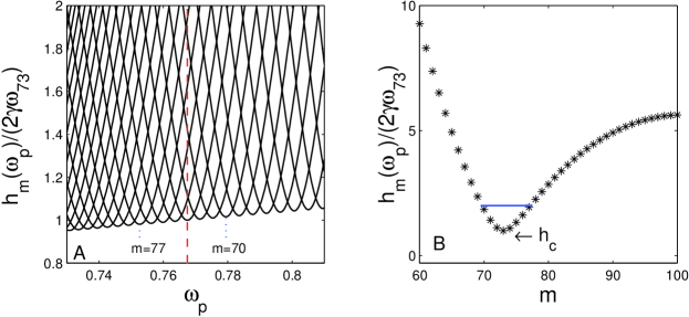
Figure 3.2: (A) A set of overlapping instability tongues $h_{m}(\omega_{p})$ for an array of $100$ oscillators as function of $\omega_{p}$. Modes $64<m<81$ are plotted, the dashed vertical line indicates the value of $\omega_{p}$ used in B. (B) Neutral stability curve as a function of mode number $m$, plotted for $\omega_{p}=\omega_{73}$. Marks the minimal driving amplitude $h_{m}(\omega_{p})$ required to excite the $m^{th}$ mode from the zero-displacement state. The horizontal line indicates the band of unstable modes for a particular value of $h=2$. The parameters used are $\Delta=0.5$ and $\epsilon\gamma=0.01$.

Chapter 4 The Response of Large Arrays - The Amplitude Equation Approach

In order to study arrays with a large number of beams, we adopt an approach usually applied to continuous spatially-extended systems. In such systems the emergence of modes, accessible from the unstable band, appear as modulations of the basic pattern determined by the initial unstable mode $q_{c}$. These modulations develop slowly over long spatial scales and thus can be described by an envelope function of the basic pattern whose dynamics obeys an appropriate set of amplitude equations [22].

4.1 Derivation of The Amplitude Equations

The general form of the amplitude equations can be deduced from symmetry considerations, but here we wish to derive the equations explicitly and obtain exact expressions for all the coefficients, that can subsequently be tested quantitatively both numerically and experimentally. We introduce a continuous displacement field $u(x,t)$, keeping in mind that only for integral values $n$ of the spatial coordinate does it actually correspond to the displacements $u(x=n,t)=u_{n}(t)$ of the discrete set of oscillators in the array. We also introduce slow spatial and temporal scales, $X=\epsilon x$ and $T=\epsilon t$, upon which the dynamics of the envelope function occurs, and expand the displacement field in terms of $\epsilon$,

$$u=\epsilon^{1/2}u^{(0)}(x,t,X,T)+\epsilon^{3/2}u^{(1)}(x,t,X,T)+O(\epsilon^{5/2}).$$ (4.1)

In order to substitute the expansion (4.1) into the equations of motion (2.4) we must express the temporal and spatial operators in Eq. (2.4) in terms of the new variables $T$ and $X$. The time derivative substitution is given by Eq. (3.5). The displacement of the $n\pm 1$ beam is given by

$$u_{n\pm 1}(t)=\epsilon^{1/2}u^{(0)}(x\pm 1,t,X,T)+O(\epsilon^{3/2}).$$ (4.2)

We insert Eqs. (3.5),(4.1) and (4.2) into (2.4), and collect terms of the same order of $\epsilon$. The $\epsilon^{1/2}$ terms yield

$$\mathfrak{L}u^{(0)}=0,\qquad\mathfrak{L}\equiv\partial_{tt}^{2}+\frac{1}{2}\Delta^{2}\left(e^{\partial_{x}}+e^{-\partial_{x}}-2\right)+1,$$ (4.3)

where $e^{\partial_{x}}$ is an operator that performs a spatial shift by $1$, thus the full spatial operator in Eq. (4.3) is simply the discrete Laplacian. Eq. (4.3) is solved by setting

$$u^{(0)}(x,t,X,T)=\left(A_{+}(X,T)e^{-iq_{p}x}+A_{-}^{*}(X,T)e^{iq_{p}x}\right)e^{i\omega_{p}t}+c.c.$$ (4.4)

The response to the lowest order of $\epsilon$ is therefore expressed in terms of two counter-propagating waves with modulated complex amplitudes $A_{+}$ and $A_{-}$. This is a typical ansatz for parametrically excited systems, though the choice of the scaling of $X$ and $T$ with $\epsilon$ is not. The asterisk and $c.c.$ stand for the complex conjugate and $q_{p}$ is determined by the driving frequency $\omega_{p}$ and the dispersion relation (3.3)

$$q_{p}=2\arcsin\sqrt{\frac{1-\omega_{p}^{2}}{2\Delta^{2}}}.$$ (4.5)

In order to obtain the $\epsilon^{3/2}$ order contribution to the different terms in the equations of motion, we express the $O(\epsilon^{3/2})$ correction of Eq. (4.2) in terms of $u^{(1)}$ and $A_{\pm}$ using the substitution

$$A_{\pm}(X+\epsilon,T)\simeq A_{\pm}(X,T)+\epsilon\frac{\partial A_{\pm}(X,T)}{\partial X}.$$ (4.6)

Using Eqs. (4.2), (4.4) and (4.6) these contributions are

$$u_{n\pm 1}:$$

$$\quad u^{(1)}(x\pm 1,t)\pm\left(\frac{\partial A_{+}}{\partial X}e^{-iq_{p}x}e^{\mp iq_{p}}+\frac{\partial A_{-}^{*}}{\partial X}e^{iq_{p}x}e^{\pm iq_{p}}\right)e^{i\omega_{p}t}+c.c.\,;$$ (4.7a)

$$u_{n+1}+u_{n-1}-2u_{n}:$$

$$\quad u^{(1)}(x+1,t)+u^{(1)}(x-1,t)-2u^{(1)}(x,t)$$

$$\quad+(e^{-iq_{p}}-e^{iq_{p}})\left(\frac{\partial A_{+}}{\partial X}e^{-iq_{p}x}-\frac{\partial A_{-}^{*}}{\partial X}e^{iq_{p}x}\right)e^{i\omega_{p}t}+c.c.$$

$$=u^{(1)}(x+1,t)+u^{(1)}(x-1,t)-2u^{(1)}(x,t)$$

$$\quad-2i\sin(q_{p})\left(\frac{\partial A_{+}}{\partial X}e^{-iq_{p}x}-\frac{\partial A_{-}^{*}}{\partial X}e^{iq_{p}x}\right)e^{i\omega_{p}t}+c.c.\,;$$ (4.7b)

$$\epsilon(\dot{u}_{n+1}+\dot{u}_{n-1}-2\dot{u}_{n}):$$

$$\quad-4i\omega_{p}\sin^{2}(q_{p}/2)\left(A_{+}e^{-iq_{p}x}+A_{-}^{*}e^{iq_{p}x}\right)e^{i\omega_{p}t}+c.c.\,;$$ (4.7c)

$$\epsilon\cos(2\omega_{p}t)(u_{n+1}+u_{n-1}-2u_{n}):$$

$$\quad-2\sin^{2}(q_{p}/2)\left(A_{+}e^{-iq_{p}x}+A_{-}^{*}e^{iq_{p}x}\right)e^{i(2\omega_{p}+\omega_{p})t}$$

$$\quad-2\sin^{2}(q_{p}/2)\left(A_{+}^{*}e^{iq_{p}x}+A_{-}e^{-iq_{p}x}\right)e^{i(2\omega_{p}-\omega_{p})t}+c.c.\,;$$ (4.7d)

$$u_{n}^{3}:$$

$$\quad\;3|A_{+}e^{-iq_{p}x}+A_{-}^{*}e^{iq_{p}x}|^{2}\left(A_{+}e^{-iq_{p}x}+A_{-}^{*}e^{iq_{p}x}\right)e^{i\omega_{p}t}+O\left(e^{i3\omega_{p}t},e^{i3q_{p}x}\right)+c.c.$$

$$=3(|A_{+}|^{2}+2|A_{-}|^{2})A_{+}e^{-iq_{p}x}e^{i\omega_{p}t}+3(2|A_{+}|^{2}+|A_{-}|^{2})A_{-}^{*}e^{iq_{p}x}e^{i\omega_{p}t}$$

$$\quad+O\left(e^{i3\omega_{p}t},e^{i3q_{p}x}\right)+c.c.\,;$$ (4.7e)

$$(u_{n\pm 1}-u_{n})^{2}(\dot{u}_{n\pm 1}-\dot{u}_{n})=\frac{1}{3}\frac{d}{dt}(u_{n\pm 1}-u_{n})^{3}:$$

$$\quad\;\frac{1}{3}\frac{d}{dt}\left((A_{+}e^{-iq_{p}x}(e^{\mp iq_{p}}-1)+A_{-}^{*}e^{iq_{p}x}(e^{\pm iq_{p}}-1))e^{i\omega_{p}t}+c.c.\right)^{3}$$

$$=\frac{d}{dt}|A_{+}e^{-iq_{p}x}(e^{\mp iq_{p}}-1)+A_{-}^{*}e^{iq_{p}x}(e^{\pm iq_{p}}-1)|^{2}$$

$$\quad\;\times\left(A_{+}e^{-iq_{p}x}(e^{\mp iq_{p}}-1)+A_{-}^{*}e^{iq_{p}x}(e^{\pm iq_{p}}-1)\right)e^{i\omega_{p}t}+O(e^{i3\omega_{p}t},e^{i3q_{p}x})+c.c.$$

$$=i\omega_{p}\left[\vphantom{A_{-}^{*}e^{i2q_{p}x}}\right.|e^{-iq_{p}}-1|^{2}(|A_{+}|^{2}+|A_{-}|^{2})+A_{+}A_{-}e^{-i2q_{p}x}(e^{\mp iq_{p}}-1)^{2}$$

$$\quad\;+A_{+}^{*}A_{-}^{*}e^{i2q_{p}x}(e^{\pm iq_{p}}-1)^{2}\left.\vphantom{A_{-}^{*}e^{i2q_{p}x}}\right]\left(A_{+}e^{-iq_{p}x}(e^{\mp iq_{p}}-1)+A_{-}^{*}e^{iq_{p}x}(e^{\pm iq_{p}}-1)\right)e^{i\omega_{p}t}$$

$$\quad\;+O(e^{i3\omega_{p}t},e^{i3q_{p}x})+c.c.\,;$$ (4.7f)

$${\rm and}$$

$$(u_{n+1}-u_{n})^{2}(\dot{u}_{n+1}-\dot{u}_{n})+(u_{n-1}-u_{n})^{2}(\dot{u}_{n-1}-\dot{u}_{n}):$$

$$\quad\;i\omega_{p}|e^{-iq_{p}}-1|^{2}(e^{iq_{p}}+e^{-iq_{p}}-2)(|A_{+}|^{2}+2|A_{-}|^{2})A_{+}e^{-iq_{p}x}e^{i\omega_{p}t}$$

$$\quad\;+i\omega_{p}|e^{-iq_{p}}-1|^{2}(e^{iq_{p}}+e^{-iq_{p}}-2)(2|A_{+}|^{2}+|A_{-}|^{2})A_{-}^{*}e^{iq_{p}x}e^{i\omega_{p}t}$$

$$\quad\;+O(e^{i3\omega_{p}t},e^{i3q_{p}x})+c.c.$$

$$=-i16\omega_{p}\sin^{4}(q_{p}/2)\left[\vphantom{A_{-}^{*}e^{i2q_{p}x}}\right.(|A_{+}|^{2}+2|A_{-}|^{2})A_{+}e^{-iq_{p}x}e^{i\omega_{p}t}+$$ (4.7g)

$$\quad\;\left.(2|A_{+}|^{2}+|A_{-}|^{2})A_{-}^{*}e^{iq_{p}x}e^{i\omega_{p}t}\right]+O(e^{i3\omega_{p}t},e^{i3q_{p}x})+c.c.\,,$$

where $O(e^{i3\omega_{p}t},e^{i3q_{p}x})$ are terms proportional to $e^{i3\omega_{p}t}$ or $e^{i3q_{p}x}$ which do not enter the dynamics at the lowest order of the $\epsilon$ expansion. The $\epsilon^{3/2}$ order terms of the equations of motion (2.4) therefore yield

$$\mathfrak{L}u^{(1)} = f$$

$$= \left[-2i\omega_{p}\left(\frac{\partial A_{+}}{\partial T}e^{-iq_{p}x}+\frac{\partial A_{-}^{*}}{\partial T}e^{iq_{p}x}\right)+i\sin(q_{p})\Delta^{2}\left(\frac{\partial A_{+}}{\partial X}e^{-iq_{p}x}-\frac{\partial A_{-}^{*}}{\partial X}e^{iq_{p}x}\right)\right]e^{i\omega_{p}t}$$

$$+\left[h\left(A_{+}^{*}e^{iq_{p}x}+A_{-}e^{-iq_{p}x}\right)-i2\omega_{p}\gamma\left(A_{+}e^{-iq_{p}x}+A_{-}^{*}e^{iq_{p}x}\right)\right]\sin^{2}(q_{p}/2)e^{i\omega_{p}t}$$

$$-\left(3+i8\eta\omega_{p}\sin^{4}(q_{p}/2)\right)\left(|A_{+}|^{2}+2|A_{-}|^{2}\right)A_{+}e^{-iq_{p}x}e^{i\omega_{p}t}$$

$$-\left(3+i8\eta\omega_{p}\sin^{4}(q_{p}/2)\right)\left(2|A_{+}|^{2}+|A_{-}|^{2}\right)A_{-}^{*}e^{iq_{p}x}e^{i\omega_{p}t}+O(e^{i3\omega_{p}t},e^{i3q_{p}x})+c.c.$$

Let us denote by $V_{0}$ the zero eigenvectors of the self adjoint operator $\mathfrak{L}$, namely, $e^{-i(q_{p}x-\omega_{p}t)}$ and $e^{i(q_{p}x+\omega_{p}t)}$ and their complex conjugates. If $u^{(1)}$ is a solution of Eq. (4.1), then $f$ must be orthogonal to the zero eigenvectors because

$$(f,V_{0})=(\mathfrak{L}u^{(1)},V_{0})=(u^{(1)},\mathfrak{L}V_{0})=0,$$ (4.9)

where $(f,g)\propto\int f(x,t)g^{*}(x,t)dxdt$ is the inner product of the $L_{2}(\mathbb{C})$ space. The Fredholm alternative theorem [23] states that Eq. (4.9) is also a sufficient condition for the existence of a solution $u^{(1)}$ for Eq. (4.1). Thus the solvability condition of Eq. (4.1) requires that the coefficients of the zero eigenvector terms at its right hand side must vanish identically. We therefore obtain two coupled amplitude equations,

$$\frac{\partial A_{+}}{\partial T}+v_{g}\frac{\partial A_{+}}{\partial X} =-\gamma\sin^{2}(q_{p}/2)A_{+}-i\frac{h}{2\omega_{p}}\sin^{2}(q_{p}/2)A_{-}$$ (4.10a)

$$-\left(4\eta\sin^{4}(q_{p}/2)-i\frac{3}{2\omega_{p}}\right)\left(|A_{+}|^{2}+2|A_{-}|^{2}\right)A_{+},$$

$$\frac{\partial A_{-}}{\partial T}-v_{g}\frac{\partial A_{-}}{\partial X} =-\gamma\sin^{2}(q_{p}/2)A_{-}+i\frac{h}{2\omega_{p}}\sin^{2}(q_{p}/2)A_{+}$$ (4.10b)

$$-\left(4\eta\sin^{4}(q_{p}/2)+i\frac{3}{2\omega_{p}}\right)\left(2|A_{+}|^{2}+|A_{-}|^{2}\right)A_{-},$$

where $v_{g}=\frac{\partial\omega}{\partial q}=-\frac{\Delta^{2}\sin(q_{p})}{2\omega_{p}}$ is the usual group velocity. Eqs. (4.10) are two coupled complex Ginzburg-Landau equations (CGLE) [24], similar to the amplitude equations previously derived for describing Faraday waves excitations [25, 26].

4.2 Linear Stability Analysis of The Zero-Displacement State

We now wish to reexamine the stability of the zero-displacement state, using the amplitude equations (4.10) we derived. For small perturbations of the zero displacement state

$$A_{\pm}=\alpha_{\pm}(T)e^{-ikX},\qquad|\alpha_{\pm}|\ll 1,$$ (4.11)

only the linear terms of Eqs. (4.10) are considered. Thus we can write the amplitude equations in a matrix form

$$\frac{\partial}{\partial T}\left(\begin{array}[]{c}\alpha_{+}\\ \alpha_{-}\\ \end{array}\right)=\left(\begin{array}[]{cc}iv_{g}k-\gamma\sin^{2}(q_{p}/2)&-i\frac{h}{2\omega_{p}}\sin^{2}(q_{p}/2)\\ i\frac{h}{2\omega_{p}}\sin^{2}(q_{p}/2)&-iv_{g}k-\gamma\sin^{2}(q_{p}/2)\\ \end{array}\right)\left(\begin{array}[]{c}\alpha_{+}\\ \alpha_{-}\\ \end{array}\right),$$ (4.12)

describing the dynamics at the onset of modes with a wave number $q=q_{p}+\epsilon k$. The solutions of Eq. (4.12) can be expressed as linear combinations of two exponents in time, $Be^{\sigma_{+}T}$ and $De^{\sigma_{-}T}$, with growth rates $\sigma_{\pm}$ determined by the eigenvalues of the matrix in the right hand side of the equation. These are given by

$$\sigma_{\pm}(h)=-\gamma\sin^{2}(q_{p}/2)\pm\sqrt{(h\sin^{2}(q_{p}/2)/2\omega_{p})^{2}-(v_{g}k)^{2}}.$$ (4.13)

The critical amplitude $h_{k}(\omega_{p})$ required to excite oscillations with a wave number $q_{p}+\epsilon k$ is obtained by setting the larger eigenvector $\sigma_{+}(h_{k})=0$, thus

$$h_{k}(\omega_{p})=2\gamma\omega_{p}\sqrt{1+\left(\frac{v_{g}k}{\gamma\sin^{2}(q_{p}/2)}\right)^{2}}.$$ (4.14)

The minimum of $h_{k}(\omega_{p})$, $h_{c}=2\gamma\omega_{p}$, is obtained for $k=0$, i.e. the amplitude equations approach yields an initial instability with a wave number $q_{c}=q_{p}$. Comparing Eq. (4.14) with the neutral stability curve Eq. (3.12) obtained by a direct linear stability analysis of the equations of motion (2.4) reveals the scope of accuracy of the scalings we use.

For $\frac{1}{N}\ll\epsilon$, the spectrum of the normal modes can be regarded as being essentially continuous, by replacing $q_{m}$ and $\omega_{m}$ by continuous variables $q$ and $\omega$ related by a continuous dispersion relation (3.3). In this limit, with $\omega_{p}$ taken from the normal frequency band, $q_{c}$ is determined by the minimum of the continuous neutral stability curve Eq. (3.12),

$$h(\omega,\omega_{p})=2\gamma\omega\sqrt{1+\left(\frac{\omega-\omega_{p}}{\epsilon\gamma\sin^{2}(q/2)}\right)^{2}}.$$ (4.15)

Even though the beams oscillate at frequency $\omega_{p}$, the initial unstable wave number $q_{c}$ is only approximately $q_{p}$. We focus on small detunings $\Omega=2(\omega_{p}-\omega)/\epsilon\ll 1$ and expand Eq. (4.15) in $\Omega$,

$$h(\Omega,\omega_{p}) = 2\gamma(\omega_{p}-\epsilon\Omega/2)\sqrt{1+\left(\frac{\Omega}{2\gamma\sin^{2}(q/2)}\right)^{2}}$$

$$= 2\gamma(\omega_{p}-\epsilon\Omega/2)\left(1+\frac{1}{2}\left(\frac{\Omega}{2\gamma\sin^{2}(q/2)}\right)^{2}\right)+O(\Omega^{4})$$

$$= 2\gamma\omega_{p}\left(1-\frac{\epsilon\Omega}{2\omega_{p}}+\frac{1}{2}\left(\frac{\Omega}{2\gamma\sin^{2}(q/2)}\right)^{2}\right)+O(\Omega^{4},\epsilon\Omega^{3})$$

$$= 2\gamma\omega_{p}\left(1+\frac{1}{2}\left(\frac{\Omega}{2\gamma\sin^{2}(q/2)}-\frac{\epsilon\gamma\sin^{2}(q/2)}{\omega_{p}}\right)^{2}\right)-\frac{\epsilon^{2}\gamma^{3}\sin^{4}(q/2)}{2\omega_{p}}+O(\Omega^{4},\epsilon\Omega^{3}).$$

Identifying the frequency detuning with

$$\epsilon\Omega/2=\omega_{p}-\omega=|v_{g}|(q-q_{p})=\epsilon|v_{g}|k,$$ (4.17)

and comparing Eq. (4.2) with the expansion of Eq. (4.14) in small $k$ reveals that in the amplitude equation approach the wave number detuning $\epsilon k$ corresponds to $q-q_{p}$ up to $\epsilon^{2}$ order corrections. This suggests that the scaling we chose for the spatial coordinate $X=\epsilon x$ is valid for the emergence of waves with $q-q_{p}\gg\epsilon^{2}$.

For $h=h_{k}(\omega_{p})$ the two eigenvalues are $\sigma_{+}=0$ and $\sigma_{-}=-2\gamma\sin^{2}{q_{p}/2}$, with the corresponding eigenvectors being

$$V_{+}=\left(\begin{array}[]{c}1\\ e^{i\psi}\\ \end{array}\right)\quad{\rm and}\quad V_{-}=\left(\begin{array}[]{c}1\\ e^{-i\psi}\\ \end{array}\right),\quad{\rm where}\quad e^{i\psi}\equiv i\frac{\gamma\sin^{2}(q_{p}/2)-iv_{g}k}{\sqrt{\gamma^{2}\sin^{4}(q_{p}/2)+(v_{g}k)^{2}}}.$$ (4.18)

The amplitudes $B$ and $D$ can be expressed in terms of $\alpha_{\pm}$ by multiplying Eq. (4.12) by the matrix

$$\left(\begin{array}[]{cc}1&1\\ e^{i\psi}&e^{-i\psi}\\ \end{array}\right)^{-1}=\frac{i}{2\sin(\psi)}\left(\begin{array}[]{cc}e^{-i\psi}&-1\\ -e^{i\psi}&1\\ \end{array}\right)$$ (4.19)

from the left. We then obtain that $B$ and $D$ are given by

$$\left(\begin{array}[]{c}B\\ D\\ \end{array}\right)\equiv\left(\begin{array}[]{c}e^{-i\psi}\alpha_{+}-\alpha_{-}\\ -e^{i\psi}\alpha_{+}+\alpha_{-}\\ \end{array}\right),$$ (4.20)

and obey

$$\frac{\partial}{\partial T}\left(\begin{array}[]{c}B\\ D\\ \end{array}\right)=-2\gamma\sin^{2}(q_{p}/2)\left(\begin{array}[]{c}0\\ D\\ \end{array}\right),$$ (4.21)

as expected. At the onset of oscillations with a wave number $q_{p}+\epsilon k$ the linear combination $B$ becomes unstable while $D$ decays exponentially with a growth rate $\sigma_{-}=-2\gamma\sin^{2}(q_{p}/2)$, suggesting that the dynamics close to the onset of oscillations can be well described using a single complex amplitude. This is what we do in the next section.

Chapter 5 Reduction to a Single Amplitude Equation

Motivated by the linear analysis of Eqs. (4.10) preformed in chapter 4.2, we express the amplitudes $A_{\pm}$ in terms of $B$ and $D$,

$$\left(\begin{array}[]{c}A_{+}\\ A_{-}\\ \end{array}\right)=\left(\begin{array}[]{cc}1&1\\ e^{i\psi}&e^{-i\psi}\\ \end{array}\right)\left(\begin{array}[]{c}B\\ D\\ \end{array}\right).$$ (5.1)

Just above threshold $h-h_{c}\ll h_{c}$ the $D$ amplitude decays exponentially in time. After transients that last over periods of order $\Gamma^{-1}\sim\epsilon^{-1}$, the response can therefore be expressed by the $B$ amplitude only

$$\left(\begin{array}[]{c}A_{+}\\ A_{-}\\ \end{array}\right)=\left(\begin{array}[]{c}1\\ e^{i\psi}\\ \end{array}\right)B.$$ (5.2)

$B(X,T)=|B(X,T)|e^{i\varphi_{B}(X,T)}$ represents an envelope of a single standing wave as apparent from substituting (5.2) back into (4.4)

$$u^{(0)}(x,t,X,T) = \left(B(X,T)e^{-iq_{p}x}+B(X,T)^{*}e^{i(q_{p}x-\psi)}\right)e^{i\omega_{p}t}+c.c.$$ (5.3)

$$= 2|B(X,T)|\left(\cos\left(\omega_{p}t-q_{p}x+\varphi_{B}\right)+\cos\left(\omega_{p}t+q_{p}x-\varphi_{B}-\psi\right)\right)$$

$$= 4|B(X,T)|\cos(\omega_{p}t-\psi/2)\cos(q_{p}x-\varphi_{B}(X,T)-\psi/2).$$

$\psi/2$ is the temporal phase relative to the drive.

This reduction of the description of the dynamics to a single amplitude $B$ is similar to the procedure introduced by Riecke [27] for describing the onset of Faraday waves. It is typical of parametric driving, which excites a single standing wave at threshold.

5.1 Scaling of $A_{\pm}$ Just Above Threshold

We define a reduced driving amplitude $g$ by letting

$$(h-h_{c})/h_{c}\equiv g\delta,\qquad\delta\ll 1.$$ (5.4)

In order to obtain an equation, describing the relevant slow dynamics of the new amplitude $B$, we need to select the proper scaling of the original amplitudes $A_{\pm}$, as well as their spatial and temporal variables, with respect to the new small parameter $\delta$.

If the coefficient of nonlinear dissipation $\eta$ is of order of one, it is apparent from the original amplitude equations (4.10) that the cubic terms saturate the growth of the amplitudes $A_{\pm}$. However, it is physically realistic to assume that $\eta$ is small. Therefore a quintic term must enter in order to saturate the growth of the amplitudes $A_{\pm}$. This can be achieved by defining the small parameter $\delta$ with respect to the coefficient of nonlinear dissipation, letting

$$\eta=\delta^{1/2}\eta_{0},\qquad\eta_{0}\sim O(1),$$ (5.5)

and taking the amplitudes to be of order $\delta^{1/4}$.

It is apparent from Eq. (4.13) for the linear growth rates that with a drive amplitude that scales like $\delta$ the growth rate of the amplitude $B$ scales like $\delta$ as well. The bandwidth of unstable wave numbers scales as $\delta^{1/2}$, as obtained by Eq. (4.14). The new temporal and spatial scales are therefore defined by $\tau=\delta T$ and $\xi=\delta^{1/2}X$ respectively, and we finally make the ansatz that

$$\left(\begin{array}[]{c}A_{+}\\ A_{-}\\ \end{array}\right)=\delta^{1/4}\left(\begin{array}[]{c}1\\ i\\ \end{array}\right)B(\xi,\tau)+\delta^{3/4}\left(\begin{array}[]{c}w^{(1)}(X,T,\xi,\tau)\\ v^{(1)}(X,T,\xi,\tau)\\ \end{array}\right)+\delta^{5/4}\left(\begin{array}[]{c}w^{(2)}(X,T,\xi,\tau)\\ v^{(2)}(X,T,\xi,\tau)\\ \end{array}\right).$$ (5.6)

The phase $e^{i\psi}$ defined by (4.18) to the lowest order of $\delta$ is $i$, because the band of unstable wave numbers $k$ scales like $\delta^{1/2}$.

5.2 Derivation of The B Amplitude Equation

The amplitude equation for $B(\xi,\tau)$ is derived by once again using the multiple scales method. We substitute Eqs. (5.4), (5.5) and the ansatz (5.6) into the original amplitude equations (4.10), and collect terms of the same order of $\delta$. The $\delta^{1/4}$ order terms satisfy Eqs. (4.10) trivially, due to the fact that the $\delta^{1/4}$ order terms in the ansatz (5.6) were chosen according to the linear stability analysis of Eqs. (4.10) performed in section 4.2.

In order to obtain the higher order terms in $\delta$ we perform the following calculations

$$\begin{split}&|A_{+}|^{2}=\delta^{1/2}|B|^{2}+\delta(B{w^{(1)}}^{*}+B^{*}w^{(1)})\,;\\ &|A_{-}|^{2}=\delta^{1/2}|B|^{2}+\delta(iBv{{}^{(1)}}^{*}-iB^{*}v^{(1)})\,;\\ &|A_{+}|^{2}A_{+}=\delta^{3/4}|B|^{2}B+\delta^{5/4}(B^{2}{w^{(1)}}^{*}+2|B|^{2}w^{(1)})\,;\\ &|A_{-}|^{2}A_{+}=\delta^{3/4}|B|^{2}B+\delta^{5/4}(iB^{2}{v^{(1)}}^{*}-i|B|^{2}v^{(1)}+|B|^{2}w^{(1)})\,;\\ &|A_{+}|^{2}A_{-}=\delta^{3/4}|B|^{2}iB+\delta^{5/4}(iB^{2}{w^{(1)}}^{*}+i|B|^{2}w^{(1)}+|B|^{2}v^{(1)})\,;\\ &|A_{-}|^{2}A_{-}=\delta^{3/4}|B|^{2}iB+\delta^{5/4}(-B^{2}{v^{(1)}}^{*}+2|B|^{2}v^{(1)})\,;\\ &\frac{\partial A_{+}}{\partial T}=\delta^{3/4}\frac{\partial w^{(1)}}{\partial T}+\delta^{5/4}\frac{\partial w^{(2)}}{\partial T}+\delta^{5/4}\frac{\partial B}{\partial\tau}\,;\\ &\frac{\partial A_{-}}{\partial T}=\delta^{3/4}\frac{\partial v^{(1)}}{\partial T}+\delta^{5/4}\frac{\partial v^{(2)}}{\partial T}+\delta^{5/4}i\frac{\partial B}{\partial\tau}\,;\\ &\frac{\partial A_{+}}{\partial X}=\delta^{3/4}\frac{\partial w^{(1)}}{\partial X}+\delta^{3/4}\frac{\partial B}{\partial\xi}+\delta^{5/4}\frac{\partial w^{(2)}}{\partial X}+\delta^{5/4}\frac{\partial w^{(1)}}{\partial\xi}\,;\\ &\frac{\partial A_{-}}{\partial X}=\delta^{3/4}\frac{\partial v^{(1)}}{\partial X}+\delta^{3/4}i\frac{\partial B}{\partial\xi}+\delta^{5/4}\frac{\partial v^{(2)}}{\partial X}+\delta^{5/4}\frac{\partial v^{(1)}}{\partial\xi}\,.\end{split}$$ (5.7)

Collecting all the $\delta^{3/4}$ order terms of Eqs. (4.10) yields

$$\mathfrak{O}\left(\begin{array}[]{c}w^{(1)}\\ v^{(1)}\\ \end{array}\right)=\left(-v_{g}\frac{\partial B}{\partial\xi}+i\frac{9}{2\omega_{p}}|B|^{2}B\right)\left(\begin{array}[]{c}1\\ -i\\ \end{array}\right),$$ (5.8)

where $\mathfrak{O}$ is a linear operator given by

$$\mathfrak{O}\equiv\left(\begin{array}[]{cc}\partial_{T}+v_{g}\partial_{X}+\gamma\sin^{2}(q_{p}/2)&i\gamma\sin^{2}(q_{p}/2)\\ -i\gamma\sin^{2}(q_{p}/2)&\partial_{T}-v_{g}\partial_{X}+\gamma\sin^{2}(q_{p}/2)\\ \end{array}\right).$$ (5.9)

There is no solvability condition since the right hand side of Eq. (5.8) is automatically orthogonal to the zero eigenvalue of $\mathfrak{O}$, $\scriptsize\left(\begin{array}[]{c}1\\ i\\ \end{array}\right)$. The solution of Eq. (5.8) is given by

$$\left(\begin{array}[]{c}w^{(1)}\\ v^{(1)}\\ \end{array}\right)=\frac{1}{2\gamma\sin^{2}(q_{p}/2)}\left(-v_{g}\frac{\partial B}{\partial\xi}+i\frac{9}{2\omega_{p}}|B|^{2}B\right)\left(\begin{array}[]{c}1\\ -i\\ \end{array}\right).$$ (5.10)

We plug Eq. (5.10) back into Eqs. (4.10) using Eqs. (5.7), collect all the terms with $\delta^{5/4}$ and obtain

$$\left[\partial_{T}+v_{g}\partial_{X}+\gamma\sin^{2}(q_{p}/2)\right]w^{(2)}+i\gamma\sin^{2}(q_{p}/2)v^{(2)}$$

$$=-\frac{\partial B}{\partial\tau}-v_{g}\frac{\partial w^{(1)}}{\partial\xi}+\gamma\sin^{2}(q_{p}/2)gB-12\eta_{0}\sin^{4}(q_{p}/2)|B|^{2}B$$

$$\quad+i\frac{3}{2\omega_{p}}\left(B^{2}{w^{(1)}}^{*}+2|B|^{2}w^{(1)}+2iB^{2}{v^{(1)}}^{*}-2i|B|^{2}v^{(1)}+2|B|^{2}w^{(1)}\right)$$

$$=-\frac{\partial B}{\partial\tau}-\frac{v_{g}}{\gamma\sin^{2}(q_{p}/2)}\frac{\partial}{\partial\xi}\left(\frac{-v_{g}}{2}\frac{\partial B}{\partial\xi}+i\frac{9}{4\omega_{p}}|B|^{2}B\right)+\gamma\sin^{2}(q_{p}/2)gB-12\eta_{0}\sin^{4}(q_{p}/2)|B|^{2}B$$

$$\quad+i\frac{3}{2\gamma\sin^{2}(q_{p}/2)\omega_{p}}\left[B^{2}\left(\frac{-v_{g}}{2}\frac{\partial B^{*}}{\partial\xi}-i\frac{9}{4\omega_{p}}|B|^{2}B^{*}\right)+4|B|^{2}\left(\frac{-v_{g}}{2}\frac{\partial B}{\partial\xi}+i\frac{9}{4\omega_{p}}|B|^{2}B\right)\vphantom{1}\right.$$

$$\quad+2iB^{2}\left(-i\frac{v_{g}}{2}\frac{\partial B^{*}}{\partial\xi}+\frac{9}{4\omega_{p}}|B|^{2}B^{*}\right)-2i|B|^{2}\left(i\frac{v_{g}}{2}\frac{\partial B}{\partial\xi}+\frac{9}{4\omega_{p}}|B|^{2}B\right)\left.\vphantom{\frac{1}{2}}\right]$$

$$=-\frac{\partial B}{\partial\tau}+\frac{v_{g}^{2}}{2\gamma\sin^{2}(q_{p}/2)}\frac{\partial^{2}B}{\partial\xi^{2}}-i\frac{9v_{g}}{4\omega_{p}\gamma\sin^{2}(q_{p}/2)}\left(2|B|^{2}\frac{\partial B}{\partial\xi}+B^{2}\frac{\partial B^{*}}{\partial\xi}\right)+\gamma\sin^{2}(q_{p}/2)gB$$

$$\quad-12\eta_{0}\sin^{4}(q_{p}/2)|B|^{2}B+i\frac{v_{g}}{\omega_{p}\gamma\sin^{2}(q_{p}/2)}\left(-3+\frac{3}{2}\right)|B|^{2}\frac{\partial B}{\partial\xi}$$

$$\quad+i\frac{v_{g}}{\omega_{p}\gamma\sin^{2}(q_{p}/2)}\left(-\frac{3}{4}+\frac{3}{2}\right)B^{2}\frac{\partial B^{*}}{\partial\xi}+\frac{1}{\omega_{p}^{2}\gamma\sin^{2}(q_{p}/2)}\left(\frac{27}{8}-\frac{27}{2}-\frac{27}{4}+\frac{27}{4}\right)|B|^{4}B$$

$$=-\frac{\partial B}{\partial\tau}+\frac{v_{g}^{2}}{2\gamma\sin^{2}(q_{p}/2)}\frac{\partial^{2}B}{\partial\xi^{2}}+\gamma\sin^{2}(q_{p}/2)gB-12\eta_{0}\sin^{4}(q_{p}/2)|B|^{2}B$$

$$\quad-i\frac{3v_{g}}{2\omega_{p}\gamma\sin^{2}(q_{p}/2)}\left(4|B|^{2}\frac{\partial B}{\partial\xi}+B^{2}\frac{\partial B^{*}}{\partial\xi}\right)-\frac{81}{8\omega_{p}^{2}\gamma\sin^{2}(q_{p}/2)}|B|^{4}B,$$ (5.11a)

and

$$\left[\partial_{T}-v_{g}\partial_{X}+\gamma\sin^{2}(q_{p}/2)\right]v^{(2)}-i\gamma\sin^{2}(q_{p}/2)w^{(2)}$$

$$=-i\frac{\partial B}{\partial\tau}+v_{g}\frac{\partial v^{(1)}}{\partial\xi}+\gamma\sin^{2}(q_{p}/2)giB-12\eta_{0}\sin^{4}(q_{p}/2)|B|^{2}iB$$

$$\quad-i\frac{3}{2\omega_{p}}\left(2iB^{2}{w^{(1)}}^{*}+2i|B|^{2}w^{(1)}+2|B|^{2}v^{(1)}-B^{2}{v^{(1)}}^{*}+2|B|^{2}v^{(1)}\right)$$

$$=-i\frac{\partial B}{\partial\tau}-iv_{g}\frac{\partial w^{(1)}}{\partial\xi}+\gamma\sin^{2}(q_{p}/2)giB-12\eta_{0}\sin^{4}(q_{p}/2)|B|^{2}iB$$

$$\quad-i\frac{3}{2\omega_{p}}\left(2B^{2}{v^{(1)}}^{*}-2|B|^{2}v^{(1)}-4|B|^{2}iw^{(1)}-iB^{2}{w^{(1)}}^{*}\right)$$

$$=i\left[-\frac{\partial B}{\partial\tau}-v_{g}\frac{\partial w^{(1)}}{\partial\xi}+\gamma\sin^{2}(q_{p}/2)gB-12\eta_{0}\sin^{4}(q_{p}/2)|B|^{2}B\vphantom{1}\right.$$

$$\quad-i\frac{3}{2\omega_{p}}\left(-2iB^{2}{v^{(1)}}^{*}+2i|B|^{2}v^{(1)}-4|B|^{2}w^{(1)}-B^{2}{w^{(1)}}^{*}\right)\left.\vphantom{\frac{1}{2}}\right]$$

$$=i\left[-\frac{\partial B}{\partial\tau}+\frac{v_{g}^{2}}{2\gamma\sin^{2}(q_{p}/2)}\frac{\partial^{2}B}{\partial\xi^{2}}+\gamma\sin^{2}(q_{p}/2)gB-12\eta_{0}\sin^{4}(q_{p}/2)|B|^{2}B\vphantom{1}\right.$$

$$\quad-i\frac{3v_{g}}{2\omega_{p}\gamma\sin^{2}(q_{p}/2)}\left(4|B|^{2}\frac{\partial B}{\partial\xi}+B^{2}\frac{\partial B^{*}}{\partial\xi}\right)-\frac{81}{8\omega_{p}^{2}\gamma\sin^{2}(q_{p}/2)}|B|^{4}B\left.\vphantom{\frac{1}{2}}\right].$$ (5.11b)

In matrix form, these equations become

$$\mathfrak{O}\left(\begin{array}[]{c}w^{(2)}\\ v^{(2)}\\ \end{array}\right)=\left[-\frac{\partial B}{\partial\tau}+\frac{v_{g}^{2}}{2\gamma\sin^{2}(q_{p}/2)}\frac{\partial^{2}B}{\partial\xi^{2}}+\gamma\sin^{2}(q_{p}/2)gB-12\eta_{0}\sin^{4}(q_{p}/2)|B|^{2}B\vphantom{1}\right.$$ (5.14)

$$+i\frac{3(-v_{g})}{2\omega_{p}\gamma\sin^{2}(q_{p}/2)}\left(4|B|^{2}\frac{\partial B}{\partial\xi}+B^{2}\frac{\partial B^{*}}{\partial\xi}\right)-\frac{81}{8\omega_{p}^{2}\gamma\sin^{2}(q_{p}/2)}|B|^{4}B\left.\vphantom{\frac{1}{2}}\right]\left(\begin{array}[]{c}1\\ i\\ \end{array}\right).$$ (5.17)

The solvability condition of Eq. (5.14) determines the amplitude equation for $B$. Again, the Fredholm alternative theorem states that the zero eigenvalue of the operator $\mathfrak{O}$, $\scriptsize\left(\begin{array}[]{c}1\\ i\\ \end{array}\right)$, must be orthogonal to the right hand side of the equation. Therefore, $B$ must satisfy

$$\frac{\partial B}{\partial\tau}=\gamma\sin^{2}(q_{p}/2)gB+\frac{v_{g}^{2}}{2\gamma\sin^{2}(q_{p}/2)}\frac{\partial^{2}B}{\partial\xi^{2}}-12\eta_{0}\sin^{4}(q_{p}/2)|B|^{2}B\vphantom{1}\\ +i\frac{3|v_{g}|}{2\omega_{p}\gamma\sin^{2}(q_{p}/2)}\left(4|B|^{2}\frac{\partial B}{\partial\xi}+B^{2}\frac{\partial B^{*}}{\partial\xi}\right)-\frac{81}{8\omega_{p}^{2}\gamma\sin^{2}(q_{p}/2)}|B|^{4}B.$$ (5.18)

After applying one last set of rescaling transformations,

$$\begin{split}&\tau\rightarrow\frac{9}{32}\frac{1}{\omega_{p}^{2}\eta_{0}^{2}\gamma\sin^{10}\left({q_{p}/2}\right)}\tau,\qquad\xi\rightarrow\frac{3}{8}\frac{|v_{g}|}{\omega_{p}\eta_{0}\gamma\sin^{6}\left({q_{p}/2}\right)}\xi,\\ &|B|^{2}\rightarrow\frac{16}{27}\omega_{p}^{2}\eta_{0}\gamma\sin^{6}\left({q_{p}/2}\right)|B|^{2},\qquad{\rm and\ }\qquad g\rightarrow\frac{32}{9}\omega_{p}^{2}\eta_{0}^{2}\sin^{8}\left({q_{p}/2}\right)g,\end{split}$$ (5.19)

we end up with an amplitude equation governed by a single parameter,

$$\frac{\partial B}{\partial\tau}=gB+\frac{\partial^{2}B}{\partial\xi^{2}}+i\frac{2}{3}\left(4|B|^{2}\frac{\partial B}{\partial\xi}+B^{2}\frac{\partial B^{*}}{\partial\xi}\right)-2|B|^{2}B-|B|^{4}B.$$ (5.20)

This amplitude equation which captures the slow dynamics of the coupled oscillators just above the onset of the parametric oscillations, is our central result. It is a variant of the CGLE [24], supplemented with the uncommon nonlinear gradient terms. Brand et. al. [28, 29, 30] studied similar equations that appear in the theory of binary fluid mixtures. However in their work all the terms in Eq. (5.20) had complex coefficients, yielding localized solutions on which the influence of the nonlinear gradients was studied. Here we focus on extended solutions and show that the nonlinear gradient terms yield the wave number detunings of single mode solutions that, as far as we are aware of, were previously introduced by hand.

Chapter 6 Single Mode Oscillations

6.1 Single Mode Solution of The Amplitude Equation

Once we have obtained the amplitude equation (5.20) it can be used to study a variety of dynamical solutions, ranging from simple single-mode to more complicated nonlinear extended solutions, or possibly even localized solutions. Here we focus on the regime of small reduced amplitude $g$ and look upon the saturation of single-mode solutions of the form

$$B=b_{k}e^{-ik\xi},\quad{\rm with}\quad b_{k}=|b_{k}|e^{i\varphi},$$ (6.1)

corresponding to a standing wave, determined by Eq. (5.3) to be

$$u_{0}=4|b_{k}|\cos(\omega_{p}t-\pi/4)\cos(qx-\pi/4-\varphi).$$ (6.2)

The shifted wave number $q$ is given by

$$q=q_{p}+\frac{8}{3}\frac{\omega_{p}\eta_{0}\gamma\sin^{6}\left({q_{p}/2}\right)}{|v_{g}|}\epsilon\sqrt{\delta}k.$$ (6.3)

The original boundary conditions $u(0,t)=u(N+1,t)=0$ impose $\varphi=\pi/4$ and require that the wave numbers $q$ be quantized according to Eq. (3.1).

We substitute (6.1) into the amplitude equation (5.20) and obtain

$$\frac{\partial b_{k}}{\partial\tau}=\left(g-k^{2}\right)b_{k}+2(k-1)|b_{k}|^{2}b_{k}-|b_{k}|^{4}b_{k}.$$ (6.4)

From the linear terms in Eq. (6.4) we find, as expected, that for $g>k^{2}$ the zero-displacement solution is unstable to small perturbations of the form of (6.1), defining the parabolic neutral stability curve, shown as a dashed line in Fig. 6.2. The nonlinear gradients and the cubic term take the simple form $2(k-1)|b_{k}|^{2}b_{k}$. For $k<1$ these terms immediately act to saturate the growth of the amplitude assisted by the quintic term. Standing waves therefore bifurcate supercritically from the zero-displacement state. For $k>1$ the cubic terms act to increase the growth of the amplitude, and saturation is achieved only by the quintic term. Standing waves therefore bifurcate subcritically from the zero-displacement state. It should be noted that similar wave-number dependent bifurcations were also predicted and observed numerically in Faraday waves [26, 31, 32], though in these works the wave number detuning $k$ was introduced a priori and was not obtained directly from the amplitude equations. Here the detuning is a direct consequence of the nonlinear gradient terms in Eq. (5.20), and is explicitly related to the physical parameters of the system.

The saturated amplitude $|b_{k}|$, obtained by setting Eq. (6.4) to zero, is given by

$$|b_{k}|^{2}=(k-1)\pm\sqrt{(k-1)^{2}+(g-k^{2})}.$$ (6.5)

In Fig. 6.1 we plot $|b_{k}|^{2}$ as a function of $g$ for two values of $k$. The solid (dashed) lines are stable (unstable) states. For $k<1$ only the positive square root branch of Eq. (6.5) is obtained, and the amplitude of oscillations increases continuously from zero for $g>k^{2}$. A subcritical bifurcation is obtained for $k>1$, the negative square root branch is obtained in addition to the positive branch for reduced driving amplitudes ranging from $k^{2}$ down to the saddle-node point given by

$$g_{sn}=2k-1.$$ (6.6)

Since two stable solutions are obtained in this range of reduced driving amplitudes for subcritical bifurcations, the system exhibits hysteresis for quasistatic driving amplitude sweeps. Quasistatic sweeps mean that the change in the driving amplitude is much slower than the time required for transients to fade so that a steady-state is obtained between each change of the driving amplitude.

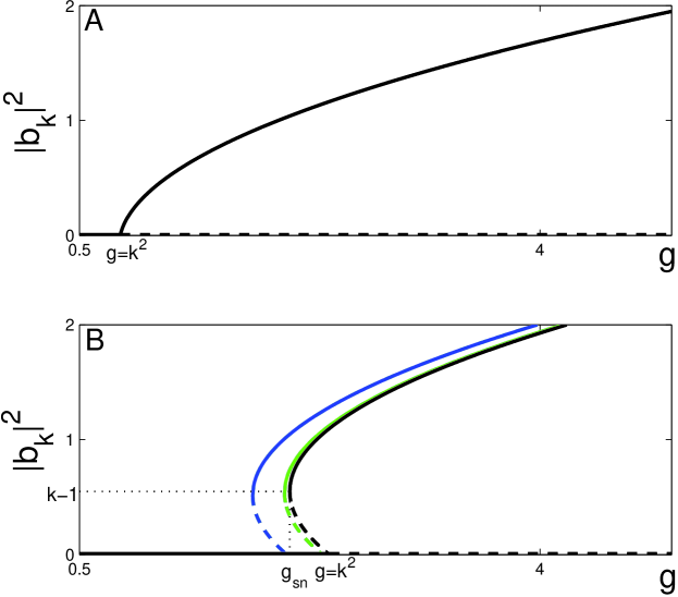
Figure 6.1: The amplitude of oscillations of the single mode state $|b_{k}|^{2}$ plotted as a function of the reduced driving amplitude g for two values of $k$. Solid and dashed black lines are the positive and negative square root branches of the calculated response in (6.5), the latter clearly unstable. (A) $k=0.9$ yields a supercritical bifurcation from the zero displacement state into the single mode state with a continuously increasing amplitude. (B) For $k=1.55$ a subcritical bifurcation occurs at $g=k^{2}$. Colored lines mark the single mode solutions calculated by Eq. (3.14) for $\epsilon=0.01$ (blue lines) and $\epsilon=0.001$ (green line). Both solutions are calculated for $\delta=0.01$ and the rest of the parameters are chosen to yield $k=1.55$. A good agreement with Eq. (6.5) is verified for $\epsilon\ll\sqrt{\delta}$.

6.2 Comparison With The Exact Form of Single Mode Solutions

We now wish to compare the exact form of single mode solutions (3.14), obtained by Lifshitz and Cross, with the solutions obtained in the previous section. In the limit of driving amplitudes just above threshold and $\eta\ll 1$, the exact amplitudes of oscillations (3.14) correspond to Eq. (6.5). The excited mode $m$ is the mode which minimizes $h_{m}(\omega_{p})$, and its wave number $q_{m}$ and frequency $\omega_{m}$ are identified (up to $O(\frac{1}{N})$ corrections) with $q_{p}$ and $\omega_{p}$ respectively. The frequency detuning $\Omega_{m}$ corresponds to $\epsilon\sqrt{\delta}v_{g}k$, with $\Omega_{c}$ equivalent to $k=1$. This implies that for a truly continuous extended system the standing waves will always bifurcate supercritically with a wave number $q_{p}$ as long as $g$ is increased quasistatically from zero. It is the discreteness of the normal modes which provides the detuning parameter essential for a subcritical bifurcation for a quasistatic increase of the driving amplitude. In Fig. 6.1 (B) we compare two exact single mode solutions calculated by Eq. (3.14) with the solution of Eq. (6.5) for $k=1.55$. It is demonstrated that the agreement between the amplitude equation approach solution and the exact solution is better for smaller $\epsilon/\sqrt{\delta}$, as discussed in section 4.2.

For frequency detunings and amplitudes of oscillations of order $\epsilon\sqrt{\delta}$, the phase obtained from Eq. (LABEL:SMb) is $\varphi=\pi/4+O(\epsilon\sqrt{\delta})$, in agreement with the phase obtained from the amplitude equation.

6.3 Secondary Instabilities

We study secondary instabilities of the single mode solutions by performing a linear stability analysis of the solution (6.1). We substitute

$$B=b_{k}e^{-ik\xi}+\left(\beta_{+}e^{-i(k+Q)\xi}+\beta_{-}^{*}e^{-i(k-Q)\xi}\right),$$ (6.7)

with $|\beta_{\pm}|\ll 1$, into the amplitude equation (5.20) and linearize in $\beta_{\pm}$. Since the amplitude equation (5.20) is invariant under phase transformations $B\rightarrow Be^{-i\varphi}$, the stability of the single mode solution cannot depend on the phase of $b_{k}$. We therefore assume that $b_{k}$ is real, and linearize the following terms of Eq. (5.20)

$$|B|^{2} \rightarrow b_{k}^{2}+b_{k}\left((\beta_{+}+\beta_{-})e^{-iQ\xi}+(\beta_{+}^{*}+\beta_{-}^{*})e^{iQ\xi}\right)\,;$$

$$B^{2} \rightarrow e^{-i2k\xi}\left(b_{k}^{2}+b_{k}\left(2\beta_{+}e^{-iQ\xi}+2\beta_{-}^{*}e^{iQ\xi}\right)\right)\,;$$

$$|B|^{4} \rightarrow b_{k}^{4}+b_{k}^{3}\left(2(\beta_{+}+\beta_{-})e^{-iQ\xi}+2(\beta_{+}^{*}+\beta_{-}^{*})e^{iQ\xi}\right)\,;$$

$$|B|^{2}B \rightarrow e^{-ik\xi}\left(b_{k}^{3}+b_{k}^{2}\left((2\beta_{+}+\beta_{-})e^{-iQ\xi}+(\beta_{+}^{*}+2\beta_{-}^{*})e^{iQ\xi}\right)\right)\,;$$

$$|B|^{4}B \rightarrow e^{-ik\xi}\left(b_{k}^{5}+b_{k}^{4}\left((3\beta_{+}+2\beta_{-})e^{-iQ\xi}+(2\beta_{+}^{*}+3\beta_{-}^{*})e^{iQ\xi}\right)\right)\,;$$

$$\frac{\partial B}{\partial\xi} \rightarrow e^{-ik\xi}\left(-ikb_{k}-i(k+Q)\beta_{+}e^{-iQ\xi}-i(k-Q)\beta_{-}^{*}e^{iQ\xi}\right)\,;$$

$$|B|^{2}\frac{\partial B}{\partial\xi} \rightarrow e^{-ik\xi}\left(-ikb_{k}^{3}-ib_{k}^{2}\left(((2k+Q)\beta_{+}+k\beta_{-})e^{-iQ\xi}+(k\beta_{+}^{*}+(2k-Q)\beta_{-}^{*})e^{iQ\xi}\right)\right)\,;$$

$$\frac{\partial B^{*}}{\partial\xi} \rightarrow e^{ik\xi}\left(ikb_{k}+i(k+Q)\beta_{+}^{*}e^{iQ\xi}+i(k-Q)\beta_{-}e^{-iQ\xi}\right)\,;$$

$$B^{2}\frac{\partial B^{*}}{\partial\xi} \rightarrow e^{-ik\xi}\left(ikb_{k}^{3}+ib_{k}^{2}\left((2k\beta_{+}+(k-Q)\beta_{-})e^{-iQ\xi}+((k+Q)\beta_{+}^{*}+2k\beta_{-}^{*})e^{iQ\xi}\right)\right).$$

The terms of order one of the equation obtained from the linearization of Eq. (5.20) recover the same Eq. (6.4) for $b_{k}$. The terms with spatial dependence of $e^{-iQ\xi}$ must satisfy

$$\begin{split}\frac{\partial\beta_{+}}{\partial\tau}&=g\beta_{+}-(k+Q)^{2}\beta_{+}+\frac{2}{3}b_{k}^{2}\left(\vphantom{{1^{1}}^{1}}4\left((2k+Q)\beta_{+}+k\beta_{-}\right)-2k\beta_{+}-(k-Q)\beta_{-}\right)\\ &\quad-2(2\beta_{+}+\beta_{-})b_{k}^{2}-(3\beta_{+}+2\beta_{-})b_{k}^{4}\\ &=\left[\vphantom{{1^{1}}^{1}}g-(k+Q)^{2}+b_{k}^{2}(4(k-1)-3b_{k}^{2}+8Q/3)\right]\beta_{+}+2b_{k}^{2}\left[\vphantom{{1^{1}}^{1}}k-1-b_{k}^{2}+Q/3\right]\beta_{-}.\end{split}$$ (6.9)

The terms with spatial dependence of $e^{iQ\xi}$ similarly obey

$$\begin{split}\frac{\partial\beta_{-}}{\partial\tau}&=g\beta_{-}-(k-Q)^{2}\beta_{-}+\frac{2}{3}b_{k}^{2}\left(\vphantom{{1^{1}}^{1}}4(k\beta_{+}+(2k-Q)\beta_{-})-(k+Q)\beta_{+}-2k\beta_{-}\right)\\ &\quad-2(\beta_{+}+2\beta_{-})b_{k}^{2}-(2\beta_{+}+3\beta_{-})b_{k}^{4}\\ &=\left[\vphantom{{1^{1}}^{1}}g-(k-Q)^{2}+b_{k}^{2}(4(k-1)-3b_{k}^{2}-8Q/3)\right]\beta_{-}+2b_{k}^{2}\left[\vphantom{{1^{1}}^{1}}k-1-b_{k}^{2}-Q/3\right]\beta_{+}.\end{split}$$ (6.10)

Using Eq. (6.5) we find that (for $\partial b_{k}/\partial\tau=0$)

$$\begin{split}g-k^{2}+4(k-1)b_{k}^{2}-3b_{k}^{4}=2b_{k}^{2}(k-1-b_{k}^{2}),\end{split}$$ (6.11)

and write Eqs. (6.9) and (6.10) in matrix form as

$$\frac{\partial}{\partial\tau}\left(\begin{array}[]{c}\beta_{+}\\ \beta_{-}\\ \end{array}\right)=M\left(\begin{array}[]{c}\beta_{+}\\ \beta_{-}\\ \end{array}\right),\quad{\rm where}$$ (6.16)

$$M\equiv\left(\begin{array}[]{cc}2b_{k}^{2}(k-1-b_{k}^{2})-Q^{2}-2Q(k-4b_{k}^{2}/3)&2b_{k}^{2}(k-1-b_{k}^{2}+Q/3)\\ 2b_{k}^{2}(k-1-b_{k}^{2}-Q/3)&2b_{k}^{2}(k-1-b_{k}^{2})-Q^{2}+2Q(k-4b_{k}^{2}/3)\\ \end{array}\right).$$ (6.19)

We express the eigenvalues of the matrix $M$ using its trace $trM$ and its determinant |M|,

$$\sigma_{\pm}=\frac{trM}{2}\pm\sqrt{\left(\frac{trM}{2}\right)^{2}-|M|}.$$ (6.20)

The single mode solution (6.1) is a stable solution only if all wave numbers $Q$ yield negative eigenvalues for $M$, obtained for $trM<0$ and $|M|>0$. A negative trace of the matrix $M$ is obtained for all wave numbers $Q$ if

$$b_{k}^{2}>k-1\qquad{\rm and}\qquad b_{k}^{2}>0.$$ (6.21)

Thus the negative square root branch in (6.5) obtained for subcritical bifurcations $k>1$, is confirmed to be always unstable. The stability of the positive square root is determined by the constraint on the determinant of $M$,

$$|M| = \left(2b_{k}^{2}(k-1-b_{k}^{2})-Q^{2}\right)^{2}-4Q^{2}(k-4b_{k}^{2}/3)^{2}-4b_{k}^{4}(k-1-b_{k}^{2})^{2}+4b_{k}^{4}Q^{2}/9$$ (6.22)

$$= Q^{4}-4Q^{2}b_{k}^{2}(k-1-b_{k}^{2})-4Q^{2}(k^{2}-8b_{k}^{2}k/3+16b_{k}^{4}/9)+4b_{k}^{4}Q^{2}/9$$

$$= \frac{8}{3}Q^{2}\left(\frac{3}{8}Q^{2}-b_{k}^{4}+\frac{5k+3}{2}b_{k}^{2}-\frac{3}{2}k^{2}\right)>0.$$

In order to obtain stable single modes, this inequality should be satisfied for all wave numbers $Q>0$ . Thus the inequality (6.22) can be replaced with

$$b_{k}^{4}-\frac{5k+3}{2}b_{k}^{2}+\frac{3}{2}k^{2}<\frac{3}{8}Q_{min}^{2},$$ (6.23)

where

$$Q_{min}\equiv\frac{3|v_{g}|}{8\omega_{p}\eta_{0}\gamma\sin^{6}(q_{p}/2)\epsilon\sqrt{\delta}}\frac{\pi}{N+1}$$ (6.24)

is the mode to mode separation in our rescaled units. Stable single mode oscillations therefore must have amplitudes obeying

$$b_{k}^{2}>0\quad{\rm for}\quad k<1,$$ (6.25a)

$$b_{k}^{2}>k-1\quad{\rm for}\quad k>1,$$ (6.25b)

$$b_{k}^{2}>\frac{5k+3}{4}-\sqrt{\left(\frac{5k+3}{4}\right)^{2}-\frac{3}{2}k^{2}+\frac{3}{8}Q_{min}^{2}},\quad{\rm and}$$ (6.25c)

$$b_{k}^{2}<\frac{5k+3}{4}+\sqrt{\left(\frac{5k+3}{4}\right)^{2}-\frac{3}{2}k^{2}+\frac{3}{8}Q_{min}^{2}}.$$ (6.25d)

The right hand side of inequality (6.25d) bounds the amplitude of stable single mode oscillations from above. The lower bound of the stable amplitudes is determined by either one of the inequalities (6.25a)-(6.25c), depending on values of $k$ and $Q_{min}$. For $k<1$ the right hand side of inequality (6.25c) determines the lower bound if

$$\frac{5k+3}{4}-\sqrt{\left(\frac{5k+3}{4}\right)^{2}-\frac{3}{2}k^{2}+\frac{3}{8}Q_{min}^{2}}>0$$

$$\Leftrightarrow\frac{3}{2}k^{2}>\frac{3}{8}Q_{min}^{2}$$

$$\Leftrightarrow|k|>\frac{Q_{min}}{2},$$ (6.26)

while for $k>1$ the condition states

$$\frac{5k+3}{4}-\sqrt{\left(\frac{5k+3}{4}\right)^{2}-\frac{3}{2}k^{2}+\frac{3}{8}Q_{min}^{2}}>k-1$$

$$\Leftrightarrow(k-1)^{2}-\frac{1}{2}(5k+3)(k-1)+\frac{3}{2}k^{2}-\frac{3}{8}Q_{min}^{2}>0$$

$$\Leftrightarrow-(k-1)\left(\frac{3}{2}k+\frac{5}{2}\right)+\frac{3}{2}k^{2}-\frac{3}{8}Q_{min}^{2}>0$$

$$\Leftrightarrow 1<k<\frac{5}{2}-\frac{3}{2}\left(\frac{Q_{min}}{2}\right)^{2}.$$

In the experimental scheme we focus on (see chapter 7) the bifurcation from the zero displacement state to single mode oscillations always occur for $|k|<Q_{min}/2$. The stability of the single mode oscillations is therefore bounded from below by (6.25a) and (6.25b). Using Eq. (6.5) we can write the boundaries of stable single mode oscillations as a function of the reduced driving amplitude $g$ and $k$. The lower bounds determined by inequalities (6.25a) and (6.25b) then take the simple form

$$g=k^{2}\quad{\rm and}\quad g=2k-1$$ (6.28)

respectively. We thus obtain that for a supercritical (subcritical) bifurcation, the positive square root branch of Eq. (6.5) is stable for reduced driving amplitudes $g$ just above the neutral stability (saddle-node) point. In Fig. 6.2 we show the stability boundaries of single mode oscillations in the $(g,k)$ plane, describing the so-called stability balloon [22] of the single mode state. The solid black curve is the stability balloon obtained for a particular set of parameters, such that $Q_{min}/2>1$, and thus it is bounded from bellow by Eqs. (6.28). Outside the curve the oscillations undergo instabilities with $Q=Q_{min}$. In the limit of very large arrays $Q_{min}\rightarrow 0$, thus the single-mode state is unstable towards perturbations with $Q\rightarrow 0$, typical of Eckhaus [33] instabilities in extended systems. In this limit the stability balloon shrinks to the blue curve in Fig.6.2.

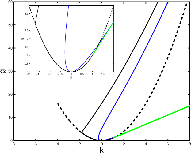
Figure 6.2: Stability boundaries of the single-mode solution of the amplitude equation (5.20) in the $g$ vs. $k$ plane. Dashed line: neutral stability boundary $g=k^{2}$. Solid lines: stability boundary of the single-mode solution (6.1) as obtained by Eqs. (6.25) for a continuous spectrum (blue curve) and for $N=92$ with the same parameters given in section 7.1 (black curve). Green line: saddle node point for the subcritical bifurcation $g_{sn}=2k-1$ which coincides with the discrete stability boundary for $k>1$.

Chapter 7 Numerical Simulations of Possible Experiments

The purpose of our numerical work is twofold: to test our analytical predictions and to simulate possible experiments that may verify our results. The equations of motion (2.4) are integrated numerically using the fourth-order Runge-Kutta method. Most of our numerical simulations mimic an experiment in which the ac component $H$ is increased quasistatically from zero, until moderate oscillations are obtained, and then swept back to zero. This is done by fixing the parameters $\Gamma,\;\Delta,\;\omega_{p},\;\eta$ and the number of oscillators in the array $N$, and scanning the values of $H$. Starting with driving amplitudes lower than the threshold $2\epsilon\gamma\omega_{p}/\Delta^{2}$, the initial conditions are taken to be those of the zero-displacement state $u_{n}(t=0)=\dot{u}_{n}(t=0)=0$ for all $n$, superimposed with small random noise. The displacements of the beams $u_{n}(t)$ develop in time according to the equations of motion (2.4). Once a steady state is obtained, the time average of the squared amplitude of each beam is calculated. The driving amplitude $H$ is then increased, and the equations are integrated for the new $H$, using the displacements and velocities of the beams just before $H$ was increased as the new initial conditions. Again a small random noise is added to the initial conditions in order to prevent the system from staying on an unstable solution of the equations, solutions which are not accessible in experiment. By repeating this procedure for increasing drives, the amplitude of oscillations as a function of the driving amplitude is obtained, and by switching to decreasing sweeps of $H$ after the array is excited, the hysteretic character of subcritical bifurcations can be observed.

We test numerically our two main predictions of the amplitude equation (5.20): the existence of a wave-number dependent bifurcation and the stability boundaries of single mode oscillations.

7.1 Wave-Number Dependent Bifurcation

The first mode to emerge when increasing the driving amplitude from $H=0$ is the mode which minimizes Eq. (3.12), whose wave number $q_{m}$ is the closest to $q_{p}$ among the spectrum of vibrational modes. In order to obtain the influence of the wave number detuning $k$ on the type of bifurcation from a zero-displacement state to single-mode oscillations, the experimenter must have a way to control $q_{m}$. By changing the number of oscillators $N$ in the array, the spectrum of vibrational modes can be modified, yielding different wave number detunings for the same driving frequency $\omega_{p}$. Since $q_{m}$ and $q_{p}$ can differ by up to $\pi/(N+1)$, $|k|$ is bounded from above by

$$|k|<\frac{Q_{min}}{2},$$ (7.1)

where $Q_{min}$ is given by Eq. (6.24). In the limit of vary large arrays $N\rightarrow\infty$, $q_{m}\rightarrow q_{p}$ and the bifurcations are always supercritical. Thus if one wants to prevent hysteresis effects in an experiment, large arrays should be considered. The weaker the dissipation of the system, the larger the array should be. For smaller arrays such that $Q_{min}\gtrsim 2$, either supercritical bifurcations $(k<1)$ or subcritical bifurcations $(k>1)$ can be obtained, depending on the specific values of $\omega_{p}$ and $\Delta$.

Our analytical treatment is valid for $\epsilon,\delta\ll 1$ and $N\gg 1$. We therefore choose to integrate arrays of about $100$ oscillators with dissipation coefficients $\Gamma=0.01$ and $\eta=0.1$, corresponding to $\epsilon=0.01$ and $\delta=0.01$ respectively. Setting the dc component to $\Delta^{2}=0.25$, ensures that the spectrum of vibrational modes satisfy $Q_{min}\simeq 2$, and thus both types of bifurcations can be obtained, depending on the number of oscillators in the array. We choose the driving frequency

$$\omega_{p}=\sqrt{1-2\Delta^{2}\sin^{2}(q_{73}/2)}=0.767445\ldots,$$ (7.2)

to obtain $q_{m}=q_{p}$ for an array of $N=100$ oscillators and a mode number $m=73$.

We numerically integrate the equations of motion (2.4) with the above parameters for arrays with $N=100$, $N=98$ and $N=92$, corresponding to wave number detunings of $k=0$, $k\simeq-0.81$ and $k\simeq 1.55$ respectively. For each array the scenario of increasing sweeps of the drive $H$ followed by decreasing sweeps as described above is performed. For each driving amplitude, the Fourier components of the steady-state solution are computed to verify that only single modes are found, suggesting that in this regime of parameters only these states are stable. In Fig. 7.1 we plot $|b_{k}|^{2}$ as a function of the reduced driving amplitude $g$ for the three wave number shifts $k$. The symbols are the numerically computed Fourier components, blue x marks are calculated for increasing driving amplitude sweeps and red circles are calculated for decreasing sweeps, showing clear hysteresis for $k>1$. The solid (dashed) lines are the stable (unstable) solutions of Eq. (6.5). The disagreement between the analytic curves and the numeric integration lies within the scope of accuracy that the amplitude equations approach as discussed previously ($g$ for instance is determined up to $O(\frac{\epsilon}{\sqrt{\delta}})\sim 0.1$).

In experiment it might be easier to control $k$ by changing the dc component of the potential difference between the beams, thus changing $q_{p}$ rather than $q_{m}$. In Fig. 7.2 we plot the response of an array of $N=100$ oscillators for two different dc components, $\Delta=0.491$ and $\Delta=0.5015$. The values of all other parameters are as given above. Changing the dc component of the potential difference might however change other parameters of the array, such as the dissipation coefficients (see chapter 1) or the coefficient of the cubic elastic restoring force [8]. In addition, a change of $q_{p}$ involves a change in the scalings performed in our analytic treatment. Thus, for the sake of simplicity we have concentrated on controlling $k$ by changing the number of oscillators $N$, but in experiment this will be difficult to do.

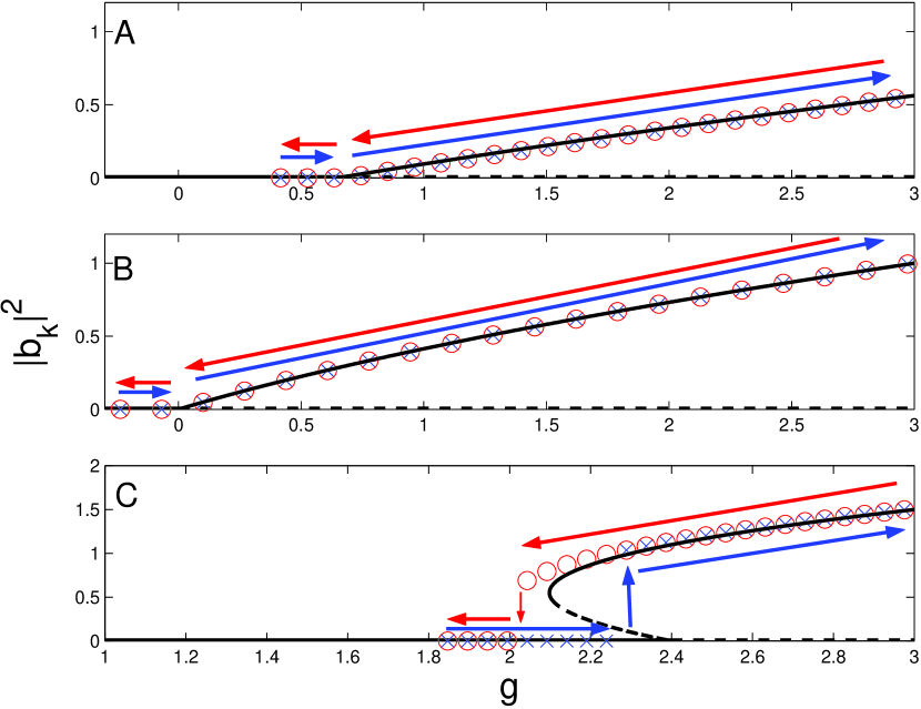
Figure 7.1: Response of the oscillator array plotted as a function of reduced amplitude $g$ for three different wave number shifts determined by fixing the number of oscillators $N$. (A) $k\simeq-0.81$ obtained for $N=92$, (B) $k=0$ obtained for $N=100$, and (C) $k\simeq 1.55$ obtained for $N=98$. Solid and dashed lines are the positive and negative square root branches of the calculated response in (6.5), the latter clearly unstable. The symbols are numerical values obtained by numerical integration of the equations of motion (2.4). Blue x-marks indicate solutions obtained for increasing sweeps of $g$, while red circles are for decreasing sweeps. The curves in (A) and (B) show a supercritical bifurcation, while that of (C) exhibits a subcritical bifurcation with clear hysteresis. The values of the parameters of the array are $\Delta=0.5$, $\omega_{p}=0.767445$, $\epsilon\gamma=0.01$ and $\eta=0.1$.

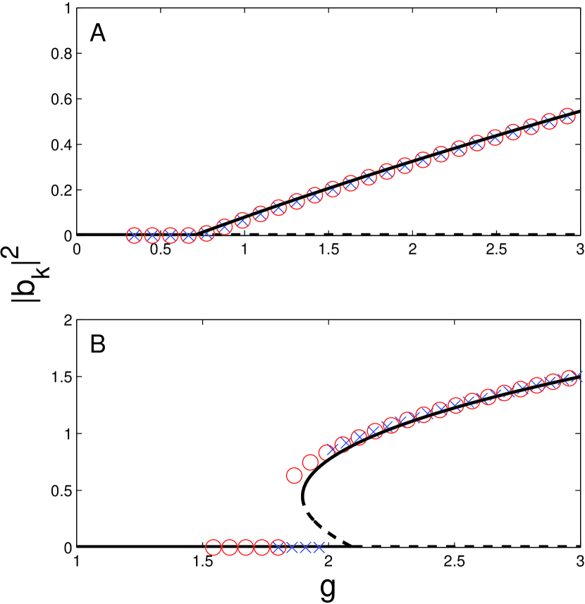
Figure 7.2: Response of an array of $N=100$ oscillators plotted as a function of reduced amplitude $g$ for two wave-number shifts determined by changing the dc component of the potential difference between the beams. (A) $k\simeq-0.84$ obtained for $\Delta=0.4991$ bifurcates supercritically, and (B) $k\simeq 1.44$ obtained for $\Delta=0.5015$ bifurcates subcritically. All other parameters are set to the same values given in Fig. 7.1.

7.2 Secondary Bifurcations

The linear stability analysis of the standing wave state performed in section 6.3 predicts a transition to a new standing wave with a wave-number shift of a multiple of $\pi/(N+1)$ once the driving amplitude is increased and has crossed the upper bound of the stability balloon. Since the upper bound monotonically increases with $k$, the new wave number will always be larger. A sequence of three transitions, obtained numerically, is shown in Fig. 7.3, superimposed with our theoretical predictions. The sequence of transitions is also sketched for comparison within the stability balloon in Fig. 7.4. All wave-number shifts obtained numerically are of $\pi/(N+1)$. Secondary instabilities are therefore another scenario for the experimental observation of hysteresis as a function of the applied driving amplitude. Once a transition has occurred, the system will return to its original state only when reducing the driving amplitude below the saddle node point.

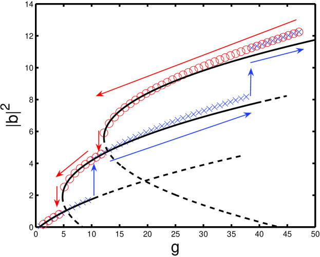
Figure 7.3: A sequence of secondary instabilities following the initial onset of single-mode oscillations in an array of $92$ beams and the same parameters given in Fig. 7.1 plotted as a function of the reduced driving amplitude $g$. Solid (dashed) lines are stable (unstable) solutions defined by (6.5), for $k=-0.81$, $k=2.90$ and $k=6.60$ corresponding to the first wave number to emerge and two shifts of the wave number by $Q_{min}$ and $2Q_{min}$ respectively. Numerical integration of the equations of motion (2.4) for an upward sweep of $g$ (blue x-marks), followed by a downward sweep (red circles) exhibits a strong hysteresis and confirms the theoretical predictions for the stability of the single mode oscillations as illustrated in Fig. 7.4.

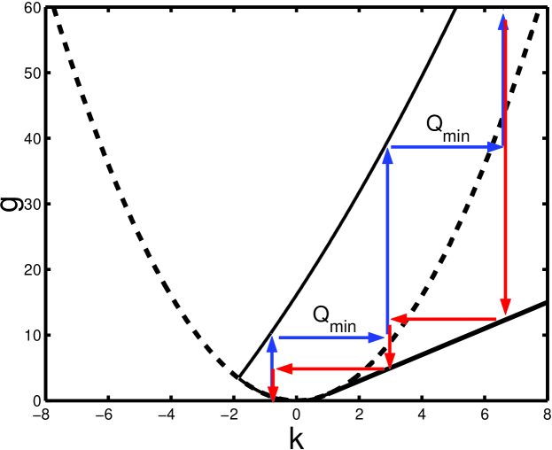
Figure 7.4: The stability balloon given in Fig. 6.2 superimposed with vertical and horizontal arrows that mark the secondary instability transitions shown in Fig. 7.3. Each transition shifts the wave-number detuning $k$ by $Q_{min}$.

Conclusions

We derived amplitude equations (4.10) describing the response of large arrays of nonlinear coupled oscillators to parametric excitation, directly from the equations of motion yielding exact expressions for all the coefficients. The dynamics at the onset of oscillations was studied by reducing these two coupled equations into a single scaled equation governed by a single control parameter. Single mode standing waves were found to be the initial states that develop just above threshold, typical of parametric excitation. The single mode oscillations bifurcate from the zero-displacement state either supercritically or subcritically, depending on the wave number of the oscillations. The wave number dependence originates in the nonlinear gradient terms of the amplitude equation, which were usually disregarded in the past by others in the analysis of parametric oscillations above threshold. We also examined the stability of single mode oscillations, predicting a transition of the initial standing wave state to a new standing wave with a larger wave number as the driving amplitude is increased.

In this work we showed that interesting response of coupled nonlinear oscillators excited parametrically can also be obtained for quasistatic driving amplitude sweeps, rather than frequency sweeps usually preformed in experiments. We proposed and numerically demonstrated two experimental schemes for observing our predictions, hoping to draw more attention of experimenters to the dynamics produced by driving amplitude sweeps.

The results obtained by the numerical integration of the equations of motion agree with our analysis, supporting the validity of the amplitude equation (5.20). We therefore believe that the amplitude equations we derived can serve as a good starting point for studying other possible states of the system. One particular interesting dynamical behavior that can be considered is that of localized modes, often observed in arrays of coupled nonlinear oscillators and in other nonlinear systems as well. The conditions for obtaining such modes and their dynamical properties could be studied by looking for localized states of the amplitude equations. Another interesting aspect that can be addressed using the amplitude equations we derived is the response of the array to fast (rather than quasistatic) driving amplitude sweeps, which should lead to more complicated nonlinear response as observed by LC in their work.

Bibliography

- [1] M. L. Roukes. Plenty of room indeed. Scientific American, 285:42, 2001.
- [2] A. N. Cleland. Foundations of Nanomechanics. Springer, Berlin, 2003.
- [3] M. P. Blencowe. Quantum electromechanical systems. Physics Reports, 395:159–222, 2004.
- [4] K. L. Turner, S. A. Miller, P. G. Hartwell, N. C. MacDonald, S. H. Strogatz, and S. G. Adams. Five parametric resonances in a microelectromechanical system. Nature, 396:149–152, 1998.
- [5] H. G. Craighead. Nanoelectromechanical systems. Science, 290:1532, 2000.
- [6] E. Buks and M. L. Roukes. Metastability and the Casimir effect in micromechanical systems. Europhys. Lett., 54:220, 2001.
- [7] D. V. Scheible, A. Erbe, and R. H. Blick. Evidence of a nanomechanical resonator being driven into chaotic response via the Ruelle-Takens route. Appl. Phys. Lett., 81:1884, 2002.
- [8] W. Zhang, R. Baskaran, and K. L. Turner. Effect of cubic nonlinearity on auto-parametrically amplified resonant mems mass sensor. Sensors and Actuators A, 102:139–150, 2002.
- [9] W. Zhang, R. Baskaran, and K. L. Turner. Tuning the dynamic behavior of parametric resonance in a micromechanical oscillator. Appl. Phys. Lett., 82:130–132, 2003.
- [10] M. Yu, G. J. Wagner, R. S. Ruoff, and M. J. Dyer. Realization of parametric resonances in a nanowire mechanical system with nanomanipulation inside a scanning electron microscope. Phys. Rev. B, 66:073406, 2002.
- [11] J. S. Aldridge and A. N. Cleland. Noise-enabled precision measurements of a duffing nanomechanical resonator. preprint (cond-mat/0406528), 2004.
- [12] D. Rugar and P. Grütter. Mechanical parametric amplification and thermomechanical noise squeezing. Phys. Rev. Lett., 67:699, 1991.
- [13] D. W. Carr, S. Evoy, L. Sekaric, H. G. Craighead, and J. M. Parpia. Parametric amplification in a torsional microresonator. Appl. Phys. Lett., 77:1545–1547, 2000.
- [14] X. M. H. Huang, C. A. Zorman, M. Mehregany, and M. L. Roukes. Nanodevice motion at microwave frequencies. Nature, 421:496, 2003.
- [15] E. Buks and M. L. Roukes. Electrically tunable collective response in a coupled micromechanical array. J. MEMS, 11:802–807, 2002.
- [16] M. Sato, B. E. Hubbard, A. J. Sievers, B. Ilic, D. A. Czaplewski, and H. G. Craighead. Observation of locked intrinsic localized vibrational modes in a micromechanical oscillator array. Phys. Rev. Lett., 90:044102, 2003.
- [17] R. Lifshitz and M. C. Cross. Response of parametrically driven nonlinear coupled oscillators with application to micromechanical and nanomechanical resonator arrays. Phys. Rev. B, 67:134302, 2003.
- [18] A. H. Nayfeh and D. T. Mook. Nonlinear Oscillations. John Wiley & Sons, New York, 3rd edition, 1995.
- [19] L. D. Landau and E. M. Lifshitz. Mechanics. Butterworth-Heinemann, Oxford, 3rd edition, 1976. §27.
- [20] S. H. Strogatz. Nonlinear dynamics and chaos, chapter 8. Westview Press, 2000.
- [21] G. Ioos and D. D. Joseph. Elementary Stability and Bifurcation Theory, chapter 2. Springer-Verlag, New York, 1980.
- [22] M. C. Cross and P. C. Hohenberg. Pattern formation outside of equilibrium. Rev. Mod. Phys., 65:851–1112, 1993.
- [23] I. Stakgold. Green’s Functions and Boundary Value Problems. John Wiley & Sons, New York, 1st edition, 1979.
- [24] I. S. Aronson and L. Kramer. The world of the complex Ginzburg-Landau equation. Rev. Mod. Phys., 74:99–143, 2002.
- [25] A. B. Ezerskiĭ, M. I. Rabinovich, V. P. Reutov, and I. M. Starobinets. Spatiotemporal chaos in the parametric excitation of capillary ripple. Zh. Eksp. Teor. Fiz., 91:2070–2083, 1986. [Sov. Phys. JETP 64, 1228 (1986)].
- [26] S. T. Milner. Square patterns and secondary instabilities in driven capillary waves. J. Fluid Mech., 225:81–100, 1991.
- [27] H. Riecke. Stable wave-number kinks in parametrically excited standing waves. Europhys. Lett., 11:213–218, 1990.
- [28] H. R. Brand, P. S. Lomdahl, and A. C. Newell. Benjamin-Feir turbulence in convective binary fluid mixtures. Physica D, 23:345–361, 1986.
- [29] H. R. Brand and R. J. Deissler. Interaction of localized solutions for subcritical bifurcations. Phys. Rev. Lett., 63:2801–2804, 1989.
- [30] R. J. Deissler and H. R. Brand. The effect of nonlinear gradient terms on localized states near weakly inverted bifurcation. Phys. Lett. A, 146:252–255, 1990.
- [31] P. Chen and K. Wu. Subcritical bifurcations and nonlinear balloons in Faraday waves. Phys. Rev. Lett., 85:3813–3816, 2000.
- [32] P. Chen. Nonlinear wave dynamics in faraday instabilities. Phys. Rev. E, 65:036308, 2002.
- [33] V. Eckhaus. Studies in Nonlinear Stability Theory, volume 6. Springer-Verlag, Berlin, 1965.