Conductance characteristics between a normal metal and a two-dimensional Fulde-Ferrell-Larkin-Ovchinnikov superconductor: the Fulde-Ferrell state

Abstract

The Fulde-Ferrell-Larkin-Ovchinnikov (FFLO) state has received renewed interest recently due to the experimental indication of its presence in CeCoIn₅, a quasi 2-dimensional (2D) $d$-wave superconductor. However direct evidence of the spatial variation of the superconducting order parameter, which is the hallmark of the FFLO state, does not yet exist. In this work we explore the possibility of detecting the phase structure of the order parameter directly using conductance spectroscopy through micro-constrictions, which probes the phase sensitive surface Andreev bound states of $d$-wave superconductors. We employ the Blonder-Tinkham-Klapwijk formalism to calculate the conductance characteristics between a normal metal (N) and a 2D $s$- or $d_{x^{2}-y^{2}}$-wave superconductor in the Fulde-Ferrell state, for all barrier parameter $z$ from the point contact limit ($z=0$) to the tunneling limit ($z\gg 1$). We find that the zero-bias conductance peak due to these surface Andreev bound states observed in the uniform $d$-wave superconductor is split and shifted in the Fulde-Ferrell state. We also clarify what weighted bulk density of states is measured by the conductance in the limit of large $z$.

I Introduction

In the early 1960’s, Fulde and Ferrell FF1964 and Larkin and Ovchinnikov LO1965 proposed the possibility that a superconducting state with a periodic spatial variation of the order parameter would become stable when a singlet superconductor is subject to a large Zeeman splitting. The Zeeman splitting could be due to either a strong magnetic field or an internal exchange field. Under such a strong magnetic or exchange field, there is a splitting of the Fermi surfaces of spin-up and -down electrons, and condensed pairs of electrons with opposite spins across the Fermi surface may be formed to lower the free energy from that of a normal spin-polarized state. These pairs have a non-zero total momentum 2q, which causes the phase of the superconducting order parameter to vary spatially with the wave number 2q. This state is known as the Fulde-Ferrell (FF) state. Larkin and Ovchinnikov (LO), on the other hand, proposed independently an alternative scenario, in which the order parameter is real, but varies periodically in space, possibly in more than one directions. Both types of states are now known (collectively) as the Fulde-Ferrell-Larkin-Ovchinnikov (FFLO) state. It has not yet been observed in conventional low-$T_{c}$ $s$-wave superconductors, which are mostly three-dimensional, probably because the orbital effect of the magnetic field dominates the Zeeman effect. The situation has been changed by experimental results suggestive of the FFLO state in heavy-fermion, quasi-1D organic, or high-$T_{c}$ superconductors; gloos ; tachiki ; modler1996a ; modler1996b ; brooks ; singleton ; mazin ; tanatar ; annett many of these compounds are quasi-one or two-dimensional, thus the orbital effect is weak when the magnetic field is in the conducting plane or along the chain. Recent experimental results in CeCoIn₅, a quasi-2D $d$-wave superconductor, are particularly encouraging. radovan ; bianchi2003 ; capan ; watanabe ; martin ; kakuyanagi ; bianchi2005 We note in passing that this subject is also of interest to the nuclear and particle physics communities because of the possible realization of the FFLO state in high density quark matter and nuclear matter, casalbuoni as well as in cold fermionic atom systems.coldatom

The most unambiguous evidence of the FFLO states should be based on phase-sensitive experiments that can directly reveal the spatial variation of the phase or sign of the order parameter. One possibility is the Josephson effect. kun2000 To the best of our knowledge there has been no report on this or other phase sensitive measurements thus far. In this paper, we consider an alternative phase sensitive probe, i.e., the conductance spectroscopy through a micro-constriction. A powerful method to calculate the differential conductance [$G(V)\equiv dI(V)/dV$] characteristics of a normal metal/superconductor junction (NSJ) was developed by Blonder, Tinkham, and Klapwijk BTK , which unified quasiparticle tunneling and Andreev reflection andreev ; deutscher . Only $s$-wave superconductors were considered in that work, but the method has since been generalized to the $d$-wave case. hu1994 ; tanaka When the sign of the order parameter experienced by the electron- and hole-like quasiparticles (QPs) before and after specular reflection at the junction interface changes, zero-energy Andreev bound states (ABSs) (also called the midgap states hu1994 ) are formed at the S side of the N/S interface (for $z\neq 0$). These ABSs will give rise to a zero-bias conductance peak (ZBCP) in the tunneling spectrum of the NSJ. A well known example of such NSJ is when the junction interface along the nodal line of the $d_{x^{2}-y^{2}}$-wave superconductor [(110) contact]. hu1994 ; tanaka ; yang ; xu ; kashiwaya ; lofwander This feature has since been widely used to identify the order-parameter symmetry of unconventional superconductors. alff ; fogelstrom ; wei1998 ; laube ; liu ; biswas ; wei2005 We would like to emphasize here that the ABSs are consequences of the phase change of the $d$-wave order parameter harlingen ; tsuei , and thus their spectra should also be sensitive to the spatial variation of the order parameter. In this paper, we will show this sensitivity by explicit calculations, and from their spectra detected via conductance spectroscopy through a micro-constriction, one can extract the momentum of the superconducting order parameter. In the present work, we will focus on the FF state; the more general LO cases are currently being investigated and will be presented elsewhere. note1 As we will show below, for a $d_{x^{2}-y^{2}}$-wave superconductor in the FF state, the ZBCP observed in a (110) contact is split and shifted by both the Zeeman field and pair momentum; the latter can be determined from the splitting.

This paper is organized as follows. In section II we introduce the model and present the self-consistent mean-field solutions for both $s$- and $d_{x^{2}-y^{2}}$-wave superconductors in the FF phases. The electron density of states (DOS) of the FF states is also obtained. The scheme to calculate the conductance characteristics is presented in section III, with numerical results for both $s$-wave and $d_{x^{2}-y^{2}}$-wave cases, and their relation with the corresponding bulk electron DOS is discussed. The features associated with the ABSs in the FF phase are explored in section IV, where we solve their spectra in the FF state. We present further discussion on our results and a summary in section V. In this work, we consider zero temperature only, and calculations on $d$-wave superconductors are simply referred to $d_{x^{2}-y^{2}}$-wave.

II The Fulde-Ferrell state and bulk density of states

We begin with the mean field Hamiltonian for a 2D superconductor in the BCS state ($\mathbf{q}=0$) or the FF state ($\mathbf{q}\neq 0$):

$$\mathcal{H}_{\mathrm{MF}}=\sum_{\mathbf{k}\sigma}(\xi_{\mathbf{k}}+\sigma\mu_{0}B)c_{\mathbf{k}\sigma}^{\dagger}c_{\mathbf{k}\sigma}{}$$ (1)

$${}-\sum_{\mathbf{k}}(\Delta_{\mathbf{kq}}c_{\mathbf{k+q}\uparrow}^{\dagger}c_{\mathbf{-k+q}\downarrow}^{\dagger}+\Delta_{\mathbf{kq}}^{\ast}c_{\mathbf{-k+q}\downarrow}c_{\mathbf{k+q}\uparrow}),$$

where $\xi_{\mathbf{k}}$ is the single-particle kinetic energy relative to the Fermi energy $\epsilon_{F}$, $B$ is the Zeeman magnetic field, $\mu_{0}$ is the magnetic moment of the electron, $\Delta_{\mathbf{kq}}$ is the pairing potential and satisfies the self-consistent condition,

$$\Delta_{\mathbf{kq}}=-\sum_{\mathbf{k^{\prime}}}V_{\mathbf{kk^{\prime}}}\langle c_{\mathbf{-k^{\prime}+q}\downarrow}c_{\mathbf{k^{\prime}+q}\uparrow}\rangle.$$ (2)

For $s$-wave, we have $V_{\mathbf{kk^{\prime}}}=-V_{0}$, while for $d$-wave, we have $V_{\mathbf{kk^{\prime}}}=-V_{0}\cos(2\theta_{\mathbf{k}})\cos(2\theta_{\mathbf{k^{\prime}}})$ (here, $|\xi_{\mathbf{k}}|,\,|\xi_{\mathbf{k^{\prime}}}|<\hbar\omega_{c}\ll\epsilon_{F}$, $\omega_{c}$ is the cutoff, $\theta_{\mathbf{k}}$ is the azimuthal angle of k). The orbital coupling between the magnetic field and electron motion is absent when the field is in the plane. The mean field Hamiltonian could be rewritten as

$$\mathcal{H}_{\mathrm{MF}}=\sum_{\mathbf{k}}(c_{\mathbf{k+q}\uparrow}^{\dagger},\,c_{\mathbf{-k+q}\downarrow})\hat{\mathrm{H}}_{\mathbf{k}}\left(\begin{array}[]{c}c_{\mathbf{k+q}\uparrow}\\ c_{\mathbf{-k+q}\downarrow}^{\dagger}\end{array}\right)+\mathrm{const.}$$ (3)

where

$$\hat{\mathrm{H}}_{\mathbf{k}}=\left(\begin{array}[]{cc}\xi_{\mathbf{k+q}}+\mu_{0}B&-\Delta_{\mathbf{kq}}\\ -\Delta_{\mathbf{kq}}^{\ast}&-\xi_{\mathbf{k-q}}+\mu_{0}B\end{array}\right).$$

To diagonalize it, we perform the Bogoliubov-Valatin transformation

$$\left(\begin{array}[]{c}c_{\mathbf{k+q}\uparrow}\\ c_{\mathbf{-k+q}\downarrow}^{\dagger}\end{array}\right)=\left(\begin{array}[]{cc}u_{\mathbf{k}}^{\ast}&v_{\mathbf{k}}\\ -v_{\mathbf{k}}^{\ast}&u_{\mathbf{k}}\end{array}\right)\left(\begin{array}[]{c}\alpha_{\mathbf{k}}\\ \beta_{\mathbf{k}}^{\dagger}\end{array}\right),$$ (4)

and choose

$$\frac{u_{\mathbf{k}}}{v_{\mathbf{k}}}=\frac{\xi_{\mathbf{k}}^{(s)}+E_{\mathbf{k}}}{\Delta_{\mathbf{kq}}},$$

$$|u_{\mathbf{k}}|^{2}=\frac{1}{2}\big{(}1+\frac{\xi_{\mathbf{k}}^{(s)}}{E_{\mathbf{k}}}\big{)}=1-|v_{\mathbf{k}}|^{2},$$

where $E_{\mathbf{k}}=\sqrt{\Delta_{\mathbf{kq}}^{2}+\xi_{\mathbf{k}}^{(s)2}}$, $\xi_{\mathbf{k}}^{(s)}=(\xi_{\mathbf{k+q}}+\xi_{\mathbf{k-q}})/2$, and $\xi_{\mathbf{k}}^{(a)}=(\xi_{\mathbf{k+q}}-\xi_{\mathbf{k-q}})/2$, from which we get the diagonalized Hamiltonian

$$\mathcal{H}_{\mathrm{MF}}=\sum_{\mathbf{k}}(E_{\mathbf{k}+}\alpha_{\mathbf{k}}^{\dagger}\alpha_{\mathbf{k}}+E_{\mathbf{k}-}\beta_{\mathbf{k}}^{\dagger}\beta_{\mathbf{k}})+\mathrm{const.}$$ (5)

with eigenenergies ($\sigma=\pm 1$)

$$E_{\mathbf{k}\sigma}=E_{\mathbf{k}}+\sigma(\mu_{0}B+\xi_{\mathbf{k}}^{(a)}).$$ (6)

There are regions in the k-space where the Cooper pairs are destroyed and occupied by electrons of one spin species; these are states with $E_{\mathbf{k}\sigma}<0$. In these cases the Bogoliubov-Valatin transformation (Eq. (4)) should be replaced by

$$\left(\begin{array}[]{c}c_{\mathbf{k+q}\uparrow}\\ c_{\mathbf{-k+q}\downarrow}^{\dagger}\end{array}\right)=\left(\begin{array}[]{cc}u_{\mathbf{k}}^{\ast}&v_{\mathbf{k}}\\ -v_{\mathbf{k}}^{\ast}&u_{\mathbf{k}}\end{array}\right)\left(\begin{array}[]{c}\alpha_{\mathbf{k}}^{\dagger}\\ \beta_{\mathbf{k}}^{\dagger}\end{array}\right)$$ (7)

when $E_{\mathbf{k}+}<0$, or

$$\left(\begin{array}[]{c}c_{\mathbf{k+q}\uparrow}\\ c_{\mathbf{-k+q}\downarrow}^{\dagger}\end{array}\right)=\left(\begin{array}[]{cc}u_{\mathbf{k}}^{\ast}&v_{\mathbf{k}}\\ -v_{\mathbf{k}}^{\ast}&u_{\mathbf{k}}\end{array}\right)\left(\begin{array}[]{c}\alpha_{\mathbf{k}}\\ \beta_{\mathbf{k}}\end{array}\right)$$ (8)

when $E_{\mathbf{k}-}<0$. note Then, the diagonalized Hamiltonian is

$$\mathcal{H}_{\mathrm{MF}}=\sum_{\mathbf{k}}(|E_{\mathbf{k}+}|\alpha_{\mathbf{k}}^{\dagger}\alpha_{\mathbf{k}}+|E_{\mathbf{k}-}|\beta_{\mathbf{k}}^{\dagger}\beta_{\mathbf{k}})+\mathrm{const.}$$ (9)

with positive quasiparticle energies.

In the weak coupling limit, the total energy of the system is given by

$$\langle\mathcal{H}-\mu N\rangle=\sum_{\mathbf{k}}\left\{\begin{array}[]{ll}2\xi_{\mathbf{k}}^{(s)}|v_{\mathbf{k}}|^{2},&E_{\mathbf{k},\pm 1}>0\\ \xi_{\mathbf{k+q}}+\mu_{0}B,&E_{\mathbf{k}+}<0\\ \xi_{\mathbf{k-q}}-\mu_{0}B,&E_{\mathbf{k}-}<0\end{array}\right\}-\frac{\Delta_{q}^{2}}{V_{0}}.$$ (10)

Here, for an $s$-wave superconductor, we have $\Delta_{\mathbf{kq}}=\Delta_{q}$, and for a $d$-wave superconductor, we have $\Delta_{\mathbf{kq}}=\Delta_{q}\cos 2\theta_{\mathbf{k}}$. For a given Zeeman field $B$, we calculate the energy of the pairing state numerically using Eq. (10) with $Q=qv_{F}/\Delta_{0}$ varied, and compare it with that of the normal spin polarized state, in order to find the ground state. In our numerical calculation presented below, we take $\hbar\omega_{c}=10\Delta_{0}$ (here $\Delta_{0}$ is the gap of the usual BCS state at $T=0$ without a Zeeman field, and for $d$-wave it is the gap along antinodal direction or maximum gap), and $H=\mu_{0}B/\Delta_{0}$. The calculation of the self-consistent pairing potential shows that the superconducting state is destroyed at $H>1$ for $s$-wave shimahara1994 and at $H>1.06$ for $d$-wave. maki1996 ; kun1998 In the superconducting regime, for $s$-wave case, at $H_{p1}\approx 0.704$, a transition occurs and the FF state becomes the ground state. For $d$-wave case, the critical Zeeman field is $H_{p1}\approx 0.544$ where an FF phase occurs with q along the nodal direction. At a higher $H_{p1}^{\prime}\approx 0.78$, the FF state with q along the antinodal direction dominates. kun1998 The critical fields $H_{p1}$ are slightly smaller than the Clogston-Chandrasekhar fields which is $H_{p1}=1/\sqrt{2}$ for $s$-wave clogston , and $\approx 0.56$ for $d$-wave kun1998 (see also Ref. vorontsov, ). The qualitative illustrations of the phase diagrams are presented in Figs. 1 and 2.

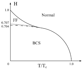
Figure 1: Qualitative sketch of the phase diagram of an $s$-wave superconductor under a Zeeman field, including the possibility of Fulde-Ferrell state. Solid line shows the phase transition between the superconducting state and the normal spin polarized state; dash-dotted line indicates the phase transition between the usual BCS state and the FF state; dotted line gives the Clogston-Chandrasekhar critical field.

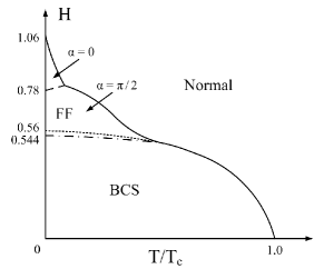
Figure 2: Qualitative sketch of the phase diagram of a $d$-wave superconductor under a Zeeman field, including the possibility of Fulde-Ferrell state. The curves have the same meaning as in Fig. 1, except that the dashed line is the phase boundary separating FF states with q along the antinodal direction and the nodal direction. Here, $\alpha$ is the angle between q and the antinodal direction.

The finite momentum of the order parameter leads to a nonzero supercurrent in the ground state. However, the supercurrent is expected to be compensated by the backflow of the quasiparticle current, and therefore, we have a zero total current. FF1964 Here we demonstrate that the total current is indeed zero for the self-consistent mean-field ground state. The total current operator can be written as

$$\mathbf{J}=\frac{e}{m}\sum_{\mathbf{k}}((\mathbf{k+q})c_{\mathbf{k+q}\uparrow}^{\dagger}c_{\mathbf{k+q}\uparrow}-(\mathbf{k-q})c_{\mathbf{-k+q}\downarrow}^{\dagger}c_{\mathbf{-k+q}\downarrow})$$ (11)

and in the superconducting state, its expectation value is

$$\langle\mathbf{J}\rangle=-\frac{e}{m}\sum_{\mathbf{k}}\left\{\begin{array}[]{ll}2\mathbf{q}|v_{\mathbf{k}}|^{2},&E_{\mathbf{k},\pm 1}>0\\ \mathbf{q+k},&E_{\mathbf{k}+}<0\\ \mathbf{q-k},&E_{\mathbf{k}-}<0\,.\end{array}\right\}.$$ (12)

By differentiate Eq. (10) at fixed $\Delta$ we can verify that

$$\langle\mathbf{J}\rangle=-e\frac{\partial}{\partial\mathbf{q}}\langle\mathcal{H}-\mu N\rangle\,.$$

Since $\langle\mathcal{H}-\mu N\rangle$ is minimized in the ${\bf q},\Delta$ space, the current must be zero.

The electron DOS can be evaluated using

$$\rho(E)=\sum_{\mathbf{k},E_{\mathbf{k}\pm}>0}|u_{\mathbf{k}}|^{2}\big{(}\delta(E-E_{\mathbf{k}+})+\delta(E-E_{\mathbf{k}-})\big{)}{}$$

$${}+\sum_{\mathbf{k},E_{\mathbf{k}+}<0}\big{(}|v_{\mathbf{k}}|^{2}\delta(E+E_{\mathbf{k}+})+|u_{\mathbf{k}}|^{2}\delta(E-E_{\mathbf{k}-})\big{)}$$

$${}+\sum_{\mathbf{k},E_{\mathbf{k}-}<0}\big{(}|u_{\mathbf{k}}|^{2}\delta(E-E_{\mathbf{k}+})+|v_{\mathbf{k}}|^{2}\delta(E+E_{\mathbf{k}-})\big{)}.$$

Within the approximation of $\xi_{\mathbf{k}}^{(s)}\approx\xi_{\mathbf{k}}$ and $\xi_{\mathbf{k}}^{(a)}\approx qv_{F}\cos(\theta_{\mathbf{k}}-\theta_{\mathbf{q}})$, it can be seen that for an arbitrary state k, there is always another state $\mathbf{k^{\prime}}$ with $\xi_{\mathbf{k^{\prime}}}=-\xi_{\mathbf{k}}$, so that both states have the same energy, and their weighting factors in Eq. II add up to unity. Thus, Eq. (II) can be simplified to

$$\rho(E) = \frac{\rho_{n}(0)}{4\pi}\int_{0}^{2\pi}d\theta\,\int_{0}^{\hbar\omega_{c}}d\xi\,\big{(}\delta(E-|E_{\mathbf{k}+}|)$$

$${}+\delta(E-|E_{\mathbf{k}-}|)\big{)},$$

where $\rho_{n}(0)$ is the DOS of the normal state at the Fermi level. Finally, we obtain

$$\frac{\rho_{e}(E)}{\rho_{n}(0)}=\frac{1}{2\pi}\int_{0}^{2\pi}d\theta\,\tilde{\rho}_{e}(E,\theta),$$ (14)

where

$$\tilde{\rho}_{e}(E,\theta)=\frac{1}{2}\Big{(}\frac{|\epsilon_{+}|}{\sqrt{\epsilon_{+}^{2}-|\Delta(\mathbf{k}_{F})|^{2}}}+\frac{|\epsilon_{-}|}{\sqrt{\epsilon_{-}^{2}-|\Delta(\mathbf{k}_{F})|^{2}}}\Big{)}\,,$$

with $\epsilon_{\sigma}=E-\sigma(\mu_{0}B+qv_{F}\cos(\theta_{\mathbf{k}}-\theta_{\mathbf{q}}))$. The result is presented in Fig. 3.

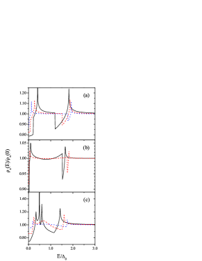
Figure 3: Representative electron density of states for various Zeeman fields and both $s$- and $d$-wave superconductors. (a) $s$-wave: solid, $H=0.704$, $Q=0.804$; dash, $H=0.8$, $Q=0.892$; dot, $H=0.9$, $Q=0.952$. (b) $d$-wave with q along the antinodal direction: solid, $H=0.78$, $Q=0.808$; dash, $H=0.88$, $Q=0.9$. (c) $d$-wave with q along the nodal direction: solid, $H=0.544$, $Q=0.608$; dash, $H=0.68$, $Q=0.816$; dot, $H=0.776$, $Q=0.94$.

III The conductance characteristics

In the presence of a normal metal/superconductor interface, to study the QPs, one needs to solve the Bogoliubov-de Gennes (BdG) equations. deGennes From the mean field Hamiltonian (1), we obtain

$$Eu_{\sigma}(\mathbf{x}) = (\hat{h}_{0}+\sigma\mu_{0}B)u_{\sigma}(\mathbf{x})$$ (15a)

$$+\int d\mathbf{x^{\prime}}\,\Delta(\mathbf{s,r})v_{\sigma}(\mathbf{x^{\prime}}),$$

$$Ev_{\sigma}(\mathbf{x}) = -(\hat{h}_{0}+\sigma\mu_{0}B)v_{\sigma}(\mathbf{x})$$ (15b)

$$+\int d\mathbf{x^{\prime}}\,\Delta^{\ast}(\mathbf{s,r})u_{\sigma}(\mathbf{x^{\prime}}),$$

where $\mathbf{s=x-x^{\prime}}$, $\mathbf{r=(x+x^{\prime})}/2$, $\hat{h}_{0}=-\nabla^{2}/2m+U\delta(x)-\mu$ and $\Delta(\mathbf{s,r})=\int d\mathbf{k}\,e^{i\mathbf{k\cdot s}}\tilde{\Delta}(\mathbf{k,r})e^{i2\mathbf{q\cdot r}}$. Here, q is determined by minimizing the ground-state energy [Eq. (10)]. To avoid accommodating super/normal current conversion at the N/S interface, which may require a nontrivial modification of the order parameter structure near the interface, we assume that q is parallel to the N/S interface at $x=0$; this choice makes theoretical analysis simpler and comparison to experiments easier. Neglecting the proximity effect at the N/S interface, we have $\tilde{\Delta}(\mathbf{k,r})=\Delta(\mathbf{k})\Theta(x)$, where $\Theta(x)$ is the step function, and $\Delta(\mathbf{k})$ is the pairing potential in the bulk superconductor. In the WKB approximation, the BdG equations have the special solutions of the form,

$$\Big{(}\begin{array}[]{c}u_{\sigma}\\ v_{\sigma}\end{array}\Big{)}=e^{i\mathbf{k}_{F}\cdot\mathbf{x}}\Big{(}\begin{array}[]{c}e^{i\mathbf{q\cdot x}}\tilde{u}_{\sigma}\\ e^{-i\mathbf{q\cdot x}}\tilde{u}_{\sigma}\end{array}\Big{)}\,,$$ (16)

where $\tilde{u}_{\sigma}$ and $\tilde{v}_{\sigma}$ obey the Andreev equations

$$\epsilon\tilde{u}_{\sigma} = -\frac{i(\mathbf{k}_{F}+\mathbf{q})}{m}\cdot\nabla\tilde{u}_{\sigma}+\Delta(\mathbf{k}_{F})\Theta(x)\tilde{v}_{\sigma},$$ (17a)

$$\epsilon\tilde{v}_{\sigma} = \frac{i(\mathbf{k}_{F}-\mathbf{q})}{m}\cdot\nabla\tilde{v}_{\sigma}+\Delta^{\ast}(\mathbf{k}_{F})\Theta(x)\tilde{u}_{\sigma},$$ (17b)

where $\epsilon=E-\sigma\mu_{0}B-\mathbf{q}\cdot\mathbf{k}_{F}/m$. The eigenenergy $E$ is symmetric about $E=\sigma\mu_{0}B+\mathbf{q}\cdot\mathbf{k}_{F}/m$ instead of zero as in Ref. BTK, . These equations are similar to those of Ref. ZTH2004, , where the authors studied conductance characteristics in the presence of a supercurrent along the junction (note that the $q/\Delta^{0}$ in Ref. ZTH2004, is equal to $Q/2$ of this work). Following the method of Blonder-Tinkham-Klapwijk BTK ; tanaka ; ZTH2004 , the normalized tunneling conductance at zero temperature is given by $G=G_{ns}/G_{nn}$, where $G_{ns}$ and $G_{nn}$ are the tunneling conductances in the superconducting and normal states, respectively. Since the QPs of the two spin species are uncoupled, the conductance will simply be the average over the two spin components:

$$G_{ns}=\frac{1}{2}(G_{ns}^{+}+G_{ns}^{-}),$$

and the same for $G_{nn}$. For simplicity, we will drop the spin index when there is no ambiguity. The conductances of each spin species are given by

$$G_{ns}=-\frac{e^{2}}{\pi}\int_{-\pi/2}^{\pi/2}d\theta\,(1+|a(-E,\theta)|^{2}-|b(E,\theta)|^{2}),$$ (18)

$$G_{nn}=-\frac{e^{2}}{\pi}\int_{-\pi/2}^{\pi/2}d\theta\,(1-|b(+\infty,\theta)|^{2}),$$ (19)

where

$$a(E,\theta)=\frac{\cos^{2}\theta}{\eta_{+}(\cos^{2}\theta+z^{2})-\eta_{-}z^{2}},$$ (20a)

$$b(E,\theta)=-\frac{z(z+i\cos\theta)(\eta_{+}-\eta_{-})}{\eta_{+}(\cos^{2}\theta+z^{2})-\eta_{-}z^{2}},$$ (20b)

$$\eta_{\pm}=\frac{\epsilon\pm\sqrt{\epsilon^{2}-|\Delta(\theta_{\pm})|^{2}}}{\Delta^{\ast}(\theta_{\pm})},$$ (20c)

$$\epsilon=E-\sigma\mu_{0}B-\frac{qk_{Fy}}{m}.$$ (20d)

Here, $a(E,\theta)$ and $b(E,\theta)$ are the Andreev and normal reflection coefficients, respectively; $\theta_{\pm}=\theta\pm\alpha$, $\theta$ is the angle between $\mathbf{k}_{F}$ and the $+x$ axis, $\alpha$ is the angle between the antinodal direction and the $+x$ axis for $d$-wave, and zero for $s$-wave, $z=mU/k_{F}$ is a dimensionless barrier-strength parameter. We give the normalized tunneling conductance of the FF states in both $s$- and $d$-wave superconductors with the arrangement of q parallel to the N/S interface in Figs. 4–6 , and also show the spin splitting effect of the tunneling conductance at a large $z=5.0$ in Fig. 7. In Fig. 8, we give the conductance of the competing uniform BCS states at the critical fields for both pair types of superconductors. Note that the Zeeman splitting for the $s$-wave case shown in Fig. 8(a) reproduces the well-known results reviewed in Ref. meservey, and the $z=0$ results given in Ref. melin, .

We start our discussion with an $s$-wave superconductor or a $d$-wave superconductor with (100) contact, where there are no ABSs; thus the conductances are determined by the bulk quasiparticles. We note that, in the arrangement considered here, due to the effect of pair momentum, the conductance curves at large $z$ seem to no longer coincide with the corresponding electron DOS for either case. [Compare Figs 4(c), 5(c), and 6(c) with Figs. 3 (a), (b), and (c).] At first sight, this appears to be against our intuitive understanding of what the NSJ conductance at high-barrier limit (tunneling limit) is supposed to be measuring; we now resolve this issue below.

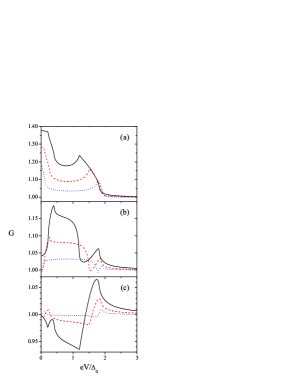
Figure 4: The normalized conductance vs voltage for normal-metal/$s$-wave FF superconductor junction: (a) $z=0$, (b) $z=0.5$, (c) $z=5.0$. Solid, $H=0.704$, $Q=0.804$; dash, $H=0.8$, $Q=0.892$; dot, $H=0.9$, $Q=0.952$.

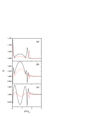
Figure 5: Same as Fig. 4 except it is now for normal-metal/$d$-wave FF superconductor junction with (100) contact. Solid, $H=0.78$, $Q=0.808$; dash, $H=0.88$, $Q=0.9$.

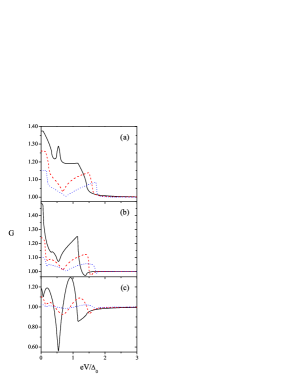
Figure 6: Same as Fig. 4 except it is now for normal-metal/$d$-wave FF superconductor junction with (110) contact. Solid, $H=0.544$, $Q=0.608$; dash, $H=0.68$, $Q=0.816$; dot, $H=0.776$, $Q=0.94$.

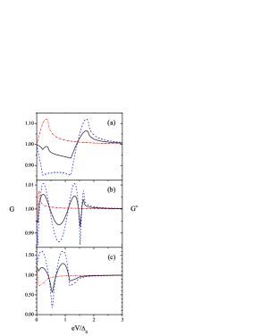
Figure 7: The normalized conductance $G$ (solid line) and its two spin components $G^{\pm}$ (dashed line for spin-up, dash-dotted line for spin-down) at a large $z=5.0$. (a) $s$-wave with $H=0.704$; (b) $d$-wave with q along antinodal direction and $H=0.78$; (c) $d$-wave with q along nodal direction and $H=0.544$.

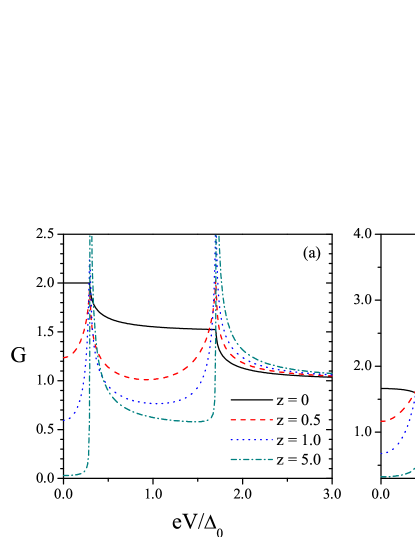
Figure 8: The normalized conductance vs voltage for the competing uniform BCS states at the critical fields with different barrier intensities $z$. (a) $s$-wave superconductor with $H=0.704$; (b) $d$-wave superconductor with $H=0.544$ and (110) contact.

In the arrangement of NSJs considered here, the applied voltage and the measured current are both along a fixed direction in the conducting plane that is normal to the N/S interface. Thus we realize that the junction conductance in the high-barrier-strength limit is actually measuring a $\cos^{2}\theta$-weighted DOS. That is, the QPs of various momenta $\bf k$ on the 2D Fermi surface (i.e., circle) do not all make equal contributions to the junction conductance, but should be weighted by $\cos^{2}\theta$ where $\theta$ is the angle between $\bf k$ and the current direction $x$. The weighted DOS [$\rho_{w}(E)$] measured in the high-$z$-limit junction conductance is therefore:

$$\frac{\rho_{w}(E)}{\rho_{n}(0)}=\frac{1}{\pi}\int_{0}^{2\pi}d\theta\,\tilde{\rho}_{e}(E,\theta)|\cos\theta|^{2}.$$ (21)

In the uniform BCS state (without involving ABSs), such weighted average simply returns to the original DOS, i.e., Eq. (21) is the same as Eq. (14) in the cases studied here. This is because the order parameter is isotropic over the momentum space for an $s$-wave superconductor, while for an N/($d$-wave superconductor) junction with (100) contact, the order parameter is symmetric about $\theta=\pm\pi/4$ so that the partial DOS of a fixed direction is also symmetric about the same line. Because the $\cos^{2}\theta$ weighting factor adds up to be 1 for two angles that are symmetric about this line, we thus have the weighted DOS by high-$z$ junction conductance to be again the same as the un-weighted DOS. tanaka However, the situation is very different in the FF state, because this kind of symmetry is broken by the pair momentum which causes a $\theta$-dependent energy shift, thus the two kinds of DOS are no longer the same. This is illustrated in Fig. 9. It is clear from this figure that the high-$z$ junction conductance measures the $\cos^{2}\theta$-weighted DOS, and not the un-weighted DOS in general. (The slight discrepancy between the tunneling conductance and the weighted DOS is because $z=5.0$ is still not high enough.)

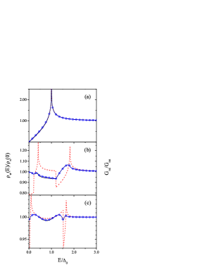
Figure 9: Comparison of the high-$z$(=5.0) junction conductance $G_{ns}$ (circles with a thin dotted line through them) with the un-weighted (dashed line) and $\cos^{2}\theta$-weighted (solid line) DOS for (a) an N/($d$-wave BCS superconductor) junction with (100) contact; (b) an N/($s$-wave FF superconductor) junction, at $H=704$; and (c) an N/($d$-wave FF superconductor) junction with (100) contact and $\bf q$ along (010), at $H=0.78$.

The most prominent features of the high-$z$ junction conductance of an N/($d$-wave FF superconductor) with (110) contact are due to the ABSs, which are the main focus of the present work. To interpret these features we need to understand how the pair momentum affects the spectra of the ABSs, which is the subject of the next section.

IV Andreev bound states in the d-wave Fulde-Ferrell superconductor with (110) junction

As has been reviewed in the introduction, for an N/($d$-wave superconductor) junction with (110) contact, a ZBCP is expected due to the formation of the “zero energy Andreev bound states” (or “midgap states”) at the junction interface. Thus for an N/($d$-wave superconductor in an FF state) junction with (110) contact and q along ($1\bar{1}0$), we need to understand the effects of $\mu_{0}B$ and q on the spectra of ABSs before we can understand the conductance characteristics for this junction.

In the limit of $z\to\infty$ we can consider a simple model with an FF superconductor in the region $x\geq 0$, and vacuum or an insulator in the region $x<0$, with q parallel to the N/S interface. In the superconductor region, from Eq. (17), we can find the solutions of bound states (which decays to zero as $x\rightarrow+\infty$) to be of the form,

$$\Big{(}\begin{array}[]{c}\tilde{u}_{\sigma\pm}\\ \tilde{v}_{\sigma\pm}\end{array}\Big{)}=e^{-\gamma x}\Big{(}\begin{array}[]{c}\hat{u}_{\sigma\pm}\\ \hat{v}_{\sigma\pm}\end{array}\Big{)}\,,$$

where

$$\gamma=m\sqrt{|\Delta|^{2}-\epsilon^{2}}/|k_{Fx}|,$$

$$\hat{u}_{\sigma\pm}/\hat{v}_{\sigma\pm}=\Delta/(\epsilon\mp i\sqrt{|\Delta|^{2}-\epsilon^{2}})\,,$$

and $\epsilon=E-\sigma\mu_{0}B-qk_{Fy}/m$ ($k_{Fx}=k_{F}\cos\theta$, $k_{Fy}=k_{F}\sin\theta$). In order to satisfy the vanishing wave-function boundary condition at $x=0$, we need to first superpose the above solutions of opposite $k_{x}$:

$$\psi_{\sigma}(\mathbf{x})=Ae^{i|k_{x}|x-\gamma x}\left(\begin{array}[]{c}e^{iqy}\hat{u}_{\sigma+}\\ e^{-iqy}\hat{v}_{\sigma+}\end{array}\right){}$$

$${}+Be^{-i|k_{x}|x-\gamma x}\left(\begin{array}[]{c}e^{iqy}\hat{u}_{\sigma-}\\ e^{-iqy}\hat{v}_{\sigma-}\end{array}\right);$$

imposing the vanishing boundary condition at $x=0$ then yields

$$\frac{\hat{u}_{\sigma+}}{\hat{v}_{\sigma+}}=\frac{\hat{u}_{\sigma-}}{\hat{v}_{\sigma-}}.$$ (24)

For an $s$-wave superconductor, and for a $d$-wave superconductor with (100) contact, Eq. (24) yields no ABSs solutions. For a $d$-wave superconductor with (110) contact, we obtain one solution for each $-k_{F}<k_{Fy}<k_{F}$ at $\epsilon=0$ or

$$E=\sigma\mu_{0}B+qk_{Fy}/m.$$ (25)

We see that the energies of the ABSs are first split by the Zeeman energy to $\sigma\mu_{0}B$ and then, shifted by an amount proportional to both the pair momentum q and the sine of the incident angle $\theta$ (which ranges between $-90^{\circ}$ and $+90^{\circ}$); the combined results of them will lead to a splitting, shifting, and broadening of the ZBCP, which we now analyze. With (110) contact, the order parameter is proportional to $\sin 2\theta$, which vanishes at $\theta=0$, and $\pm 90^{\circ}$, implying that near these special values there are either no ABSs, or their contributions to conductance will be very weak because these are very loosely bound states; the dominant contributions come from ABSs with $\theta$ around $\pm\pi/4$ (or around gap maxima); the energy shift of these states due to pair momenta are in opposite direction when the sign of $\theta$ are different. Thus for sufficiently large $q$, which is the case here, the junction conductance at positive bias should exhibit two peaks, one on each side of $\mu_{0}B$, and a dip at the Zeeman field energy $E=\mu_{0}B$. (The conductance has a symmetry about zero bias in the approximation adopted here, so we do not need to consider negative bias.) For the two peaks, the one on the right side ($E_{p+}$) arises from $0<\theta<\pi/2$, whereas the one on the left side ($E_{p-}$) arises from $-\pi/2<\theta<0$. If only spin-up QPs are considered, the two peaks are of equal strength and equal distance from the dip as illustrated in the dashed line of Fig. 7(c). When the contributions from the QPs of both spin species are summed up, the two peaks will not be symmetric about the dip ($E_{p-}$ will be shifted slightly to the right, but the influence on $E_{p+}$ and the dip is negligible), and a weak peak at zero bias emerges (see Fig. 7(c)). To locate the position of the peak $E_{p+}$, we first notice from Eqs. 18–20 that the bias voltage difference between the peak and the dip, $\delta E_{p}=|E_{p+}-\mu_{0}B|$, should be a function of $qv_{F}$ in the high-$z$ limit and vanishes when the pair momentum is zero. Numerically, therefore we can consider a simplified situation where there exists the pair momentum without Zeeman field (such in Ref. ZTH2004, ) and calculate this difference as a function of the pair momentum. The result is shown in Fig. 10. By fitting the data to a straight line through the origin, we obtain

$$E_{p+}\approx\mu_{0}B+\frac{2}{3}qv_{F}\,.$$ (26)

Thus, by measuring the bias voltages of the peak and the dip in the high-$z$ junction conductance with (110) contact, and in particular the difference between them, we can obtain a good estimate of q. We note that without this pair momentum, we would have all ABSs at energies $E=\sigma\mu_{0}B$, which would have given rise to one sharp peak only at $eV=\mu_{0}B$ in the same conductance plot, as shown in Fig. 8(b). Therefore we conclude that the signature of the FF state is clearly revealed in the junction conductance characteristics, especially at high $z$, but the conductance behaviors at low $z$ for all three cases studied here are also quite novel, since they are quite different from the corresponding results for uniform $s$- or $d$-wave superconductors.

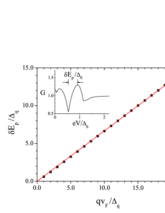
Figure 10: The bias voltage difference of the tunneling conductance peak ($E=E_{p+}$) and the dip ($E=\mu_{0}B$) at large $z$(=20), $\delta E_{p}=|E_{p+}-\mu_{0}B|$, as a function of $qv_{F}$ (both in unit of $\Delta_{q}$) for $d$-wave superconductor with (110) contact. The value range of $qv_{F}/\Delta_{q}$ is extended to 0–20, while the physical range is about 1.5–7.7. Solid line is the linear fit of the numerical data, and its slope is $0.667\pm 0.001$. The inset is an illustration of the voltage difference measured in the experiment.

V Summary and Discussion

In this paper we have studied the conductance characteristics of a junction between a normal metal and a superconductor in the Fulde-Ferrell (FF) state, using the Blonder-Tinkham-Klapwijk formalism. We have studied both $s$- and $d$-wave cases, and for the latter case, we considered junctions along both the nodal [(110)] and antinodal [(100)] directions.

The conductance characteristics of a micro-constriction is presumably easiest to understand in the high tunneling-barrier limit, when the conductance should give information about DOS of the superconductor. In the FF phase, the Zeeman field should split the contributions to the conductance by the spin-up and -down QPs, i.e., shifting their contributions by the Zeeman energy in opposite directions. In addition, for QPs of either spin species, their contributions should be shifted by an amount proportional to the pair momentum, with a proportionality constant depending on the cosine of the angle between its kinetic momentum and the pair momentum. This proportionality constant can range from a negative maximum to a positive maximum. Thus we found the effect of q to be a broadening rather than a shift. One would expect similar effects to occur on the contributions by the ABSs, resulting in the shift and broadening of the ZBCP. Thus, in the high-barrier-limit, one might (naively) expect the tunneling spectrum of $d$-wave superconductor with (110) contact to be composed of broadened ZBCP’s centered around $\pm\mu_{0}B$. In our numerical results, we find instead that the high-barrier-limit tunneling conductance of $d$-wave superconductors with (110) contact has a dip at the Zeeman energy, with one round peak on each side of it, and also another weak peak at exactly zero energy. This is quite different from the situation of the BCS state in the presence of a Zeeman field, in which case one expects the sharp ZBCP to be shifted to $\pm\mu_{0}B$, as well as the naive expectation above. The dip and the two round peaks can be understood as due to the fact that the q values appearing here are so large that they are already beyond the critical value obtained in Ref. ZTH2004, , which studied directly the current effect on the conductance characteristics in the absence of a Zeeman field. For such large q values, their effect on the ZBCP in the high-barrier-limit tunneling conductance is to split the ZBCP into two round peaks with a center dip. It is worth noting that such high values of q are not accessible through direct application of a supercurrent. The weak peak at zero energy turns out to be the result of summing up spin-up and -down contributions. Furthermore, numerical analysis shows that the bias voltage difference between the dip and the round peak on its right side is proportional to the pair momentum and thus gives us a simple way to estimate the pair momentum for $d$-wave superconductor with (110) contact.

For $s$-wave superconductor and $d$-wave superconductor with (100) contact, there is no ABS and the conductance is due to contributions from bulk quasiparticles exclusively. In these cases we have also found conductance features in the FF superconductors that are very different from the BCS superconductors. We found that because of the energy shift due to the pair momentum (which breaks the spatial symmetries in the original system), the conductance in the high barrier limit is no longer the same as the electron DOS; instead, it reflects a directionally-weighted DOS. In principle, by comparing the conductance and the bulk DOS maki2004a ; vorontsov ; mizushima ; wang that are measured by other means (such as tunneling along the $c$-direction instead of an in-plane direction discussed here), one can also distinguish between BCS and FF states.

The FF state studied here is the simplest version of the general Fulde-Ferrell-Larkin-Ovchinnikov (FFLO) superconductors. Its simplicity allows for a fairly straightforward calculation of the conductance characteristics through micro-constriction, note1 as well as an understanding of the results. Study of the conductance characteristics for general FFLO states is currently under way and will be reported elsewhere.

- (1) P. Fulde and R. A. Ferrell, Phys. Rev. 135, A550 (1964).
- (2) A. I. Larkin and Y. N. Ovchinnikov, Sov. Phys. JETP 20, 762 (1965).
- (3) K. Gloos, R. Modler, H. Schimanski, C. D. Bredl, C. Geibel, F. Steglich, A. I. Buzdin, N. Sato, and T. Komatsubara, Phys. Rev. Lett. 70, 501 (1993).
- (4) M. Tachiki, S. Takahashi, P. Gegenwart, M. Weiden, M. Lang, C. Geibel, F. Steglich, R. Modler, C. Paulsen, and Y. Onuki, Z. Phys. B: Condens. Matter 100, 369 (1996).
- (5) R. Modler, P. Gegenwart, M. Lang, M. Deppe, M. Weiden, T. Lühmann, C. Geibel, F. Steglich, C. Paulsen, J. L. Tholence, N. Sato, T. Komatsubara, Y. Onuki, M. Tachiki, and S. Takahashi, Phys. Rev. Lett. 76, 1292 (1996).
- (6) P. Gegenwart, M. Deppe, M. Koppen, F. Kromer, M. Lang, R. Modler, M. Weiden, C. Geibel, F. Steglich, T. Fukase, and N. Toyota, Ann. Phys. (Leipzig) 5, 307 (1996).
- (7) J. L. O’Brien, H. Nakagawa, A. S. Dzurak, R. G. Clark, B. E. Kane, N. E. Lumpkin, R. P. Starrett, N. Muira, E. E. Mitchell, J. D. Goettee, D. G. Rickel, and J. S. Brooks, Phys. Rev. B 61, 1584 (2000).
- (8) J. Singleton, J. A. Symington, M.-S. Nam, A. Ardavan, M. Kurmoo, and P. Day, J. Phys.: Condens. Matter 12, L641 (2000).
- (9) D. J. Singh and I. I. Mazin, Phys. Rev. Lett. 88, 187004 (2002).
- (10) M. A. Tanatar, T. Ishiguro, H. Tanaka, and H. Kobayashi, Phys. Rev. B 66, 134503 (2002).
- (11) M. Krawiec, B. L. Györffy, and J. F. Annett, Phys. Rev. B 70, 134519 (2004).
- (12) H. A. Radovan, N. A. Fortune, T. P. Murphy, S. T. Hannahs, E. C. Palm, S. W. Tozer, and D. Hall, Nature (London) 425, 51 (2003).
- (13) A. Bianchi, R. Movshovich, C. Capan, P. G. Pagliuso, and J. L. Sarrao, Phys. Rev. Lett. 91, 187004 (2003).
- (14) C. Capan, A. Bianchi, R. Movshovich, A. D. Christianson, A. Malinowski, M. F. Hundley, A. Lacerda, P. G. Pagliuso, and J. L. Sarrao, Phys. Rev. B 70, 134513 (2004).
- (15) T. Watanabe, Y. Kasahara, K. Izawa, T. Sakakibara, Y. Matsuda, C. J. van der Beek, T. Hanaguri, H. Shishido, R. Settai, and Y. Onuki, Phys. Rev. B 70, 020506 (2004).
- (16) C. Martin, C. C. Agosta, S. W. Tozer, H. A. Radovan, E. C. Palm, T. P. Murphy, and J. L. Sarrao, Phys. Rev. B 71, 020503 (2005).
- (17) K. Kakuyanagi, M. Saitoh, K. Kumagai, S. Takashima, M. Nohara, H. Takagi, and Y. Matsuda, Phys. Rev. Lett. 94, 047602 (2005).
- (18) R. Movshovich, A. Bianchi, C. Capan, P. G. Pagliuso, and J. L. Sarrao, Physica B 359, 416 (2005).
- (19) For a review, see R. Casalbuoni and G. Nardulli, Rev. Mod. Phys. 76, 263 (2004).
- (20) W. V. Liu and F. Wilczek, Phys. Rev. Lett. 90, 047002 (2003); T. Mizushima, K. Machida, and M. Ichioka., Phys. Rev. Lett. 94, 060404 (2005); K. Yang, cond-mat/0504691; A. Sedrakian, J. Mur-Petit, A. Polls, and H. Müther, Phys. Rev. A 72, 013613 (2005); C.-H. Pao, S.-T. Wu, and S.-K. Yip, cond-mat/0506437; D. T. Son and M. A. Stephanov, cond-mat/0507586; D. E. Sheehy and L. Radzihovsky, cond-mat/0508430; K. Yang, cond-mat/0508484.
- (21) K. Yang and D. F. Agterberg, Phys. Rev. Lett. 84, 4970 (2000).
- (22) G. E. Blonder, M. Tinkham, and T. M. Klapwijk, Phys. Rev. B 25, 4515 (1982).
- (23) A. F. Andreev, Zh. Eksp. Teor. Fiz. 46, 1823 (1964) [Sov. Phys. JETP 19, 1228 (1964)].
- (24) G. Deutscher, Rev. Mod. Phys. 77, 109 (2005).
- (25) C.-R. Hu, Phys. Rev. Lett 72, 1526 (1994).
- (26) Y. Tanaka and S. Kashiwaya, Phys. Rev. Lett. 74, 3451 (1995).
- (27) J. Yang and C.-R. Hu, Phys. Rev. B 50, 16766 (1994).
- (28) J. H. Xu, J. H. Miller, Jr., and C. S. Ting, Phys. Rev. B 53, 3604 (1996).
- (29) S. Kashiwaya and Y. Tanaka, Rep. Prog. Phys. 63, 1641 (2000).
- (30) T. Löfwander, V. S. Shumeiko, and G. Wendin, Supercond. Sci. Technol. 14, R53 (2001).
- (31) L. Alff, H. Takashima, S. Kashiwaya, N. Terada, H. Ihara, Y. Tanaka, M. Koyanagi, and K. Kajimura, Phys. Rev. B 55, 14757 (1997).
- (32) M. Fogelström, D. Rainer, and J. A. Sauls, Phys. Rev. Lett. 79, 281 (1997).
- (33) J. Y. T. Wei, N.-C. Yeh, D. F. Garrigus, and M. Strasik, Phys. Rev. Lett. 81, 2542 (1998).
- (34) F. Laube, G. Goll, H. v. Löhneysen, M. Fogelström, and F. Lichtenberg, Phys. Rev. Lett. 84, 1595 (2000).
- (35) Z. Q. Mao, K. D. Nelson, R. Jin, Y. Liu, and Y. Maeno Phys. Rev. Lett. 87, 037003 (2001).
- (36) A. Biswas, P. Fournier, M. M. Qazilbash, V. N. Smolyaninova, H. Balci, and R. L. Greene, Phys. Rev. Lett. 88, 207004 (2002).
- (37) P. M. C. Rourke, M. A. Tanatar, C. S. Turel, J. Berdeklis, C. Petrovic, and J. Y. T. Wei, Phys. Rev. Lett. 94, 107005 (2005).
- (38) D. J. Van Harlingen, Rev. Mod. Phys. 67, 515 (1995).
- (39) C. C. Tsuei and J. R. Kirtley, Rev. Mod. Phys. 72, 969 (2000).
- (40) In general the FF state with a single momentum for the order parameter may not be the lowest energy mean-field state of the system. However it has the advantage of being the simplest version of the more general FFLO states, and in particular the Blonder-Tinkham-Klapwijk equations for conductance can be solved analytically in closed form. It thus provides a natural starting point, and we expect the qualitative features of our results to be robust.
- (41) Note that the subscript k in the new creation operators defined in Eqs. (4) and (7) is only an index. The new QPs generated by these creation operators actually have momentum in the order of . (They are not momentum eigenstates to the accuracy of .)
- (42) H. Shimahara, Phys. Rev. B 50, 12760 (1994).
- (43) K. Maki and H. Won, Czech. J. Phys. 46, 1035 (1996).
- (44) K. Yang and S. L. Sondhi, Phys. Rev. B 57, 8566 (1998).
- (45) A. M. Clogston, Phys. Rev. Lett. 9, 266 (1962); B. S. Chandrasekhar, Appl. Phys. Lett. 1, 7 (1962).
- (46) A. B. Vorontsov, J. A. Sauls, and M. J. Graf, Phys. Rev. B 72, 184501 (2005). This work focuses on the bulk properties of LO type of states.
- (47) P. G. de Gennes, Superconductivity of metals and alloys (Perseus Books, 1999).
- (48) D. Zhang, C. S. Ting, and C.-R. Hu, Phys. Rev. B 70, 172508 (2004).
- (49) R. Meservey and P. M. Tedrow, Phys. Rep. 238, 173 (1994).
- (50) R. Mélin, Europhys. Lett. 51, 202 (2000).
- (51) H. Won, K. Maki, S. Haas, N. Oeschler, F. Weickert, and P. Gegenwart, Phys. Rev. B 69, 180504 (2004).
- (52) T. Mizushima, K. Machida, and M. Ichioka, Phys. Rev. Lett. 95, 117003 (2005).
- (53) Q. Wang, H. Y. Chen, C.-R. Hu, and C. S. Ting, Phys. Rev. Lett. 96, 117006 (2006).