Quantum chaotic patterns in the E$\otimes(b_{1}+b_{2})$ Jahn-Teller model

Abstract

We study statistical properties of excited levels of the E$\otimes(b_{1}+b_{2})$ Jahn-Teller model. The multitude of avoided crossings of energy levels is generally claimed to be a testimony of quantum chaos. We found that apart from two limiting cases ($E\otimes e$ and Holstein model) the distribution of nearest-neighbor spacings is rather stable as to the change of parameters and different from the Wigner one. This limiting distribution assumably shows scaling $\sim\sqrt{S}$ at small $S$ and resembles the semi-Poisson law $P(S)=4S\exp(-2S)$ at $S\geq 1$. The latter is believed to be universal and characteristic, e.g., at the transition between metal and insulator phases.

Phonon spectra of two-level electron systems – two phonon E$\times$e Jahn-Teller (JT) model with rotation symmetry Wagner:1992 and one-phonon exciton models Kong:1990 ; Graham:1984 ; Eidson:1986 ; Esser:1994 ; Sonnek:1994 ; Herfort:2001 show up remarkable features: multiple avoided level crossings (MAC) and localized (“exotic”) excited states at certain quantum numbers. These phenomena are typical for chaotic spectra (e.g., in complex nuclei) usually associated with underlying non-integrable Hamiltonians Eckhardt:1988 ; Nakamura:book:1993 ; Brody:1981 .

The reflection symmetric two-level Hamiltonians contain a hidden nonlinearity due to the phonon assistance of the tunneling term which reveals explicitly after the elimination of the electron degrees of freedom Wagner:1992 ; Shore:1973 ; Majernikova:2002 ; Wagner:1984 ; Majernikova:2003 . Semiclassical approaches to the phonon dynamics handle this nonlinearity in different ways. One or another decoupling method results in losing different amounts of the quantum information, and hence to controversial conclusions about possible classical chaotic behavior Graham:1984 .

The adiabatic approach to the quantum E$\times$e JT model [rotation symmetric version with two vibron (boson) modes, one symmetric and the other antisymmetric against the reflection] applies in a limited range of validity for the strong electron-phonon coupling Wagner:1992 ; Wagner:1984 . Namely, the rotational momentum $\hat{J}$ even in the ground state ($|j|=\frac{1}{2}$) mediates the coupling between levels and brings in the nonlinearity due to the reflection symmetry Wagner:1992 ; Majernikova:2002 ; Shore:1973 ; Wagner:1984 ; Majernikova:2003 . Consequently, excited spectra especially at big $|j|$ are marked by a high density of avoided level crossings Wagner:1992 . The source of both MAC and localization is the interplay of the quantum coupling of levels and nonlinearity. The asymmetry of the interaction constants $\alpha\neq\beta$ in E$\otimes(b_{1}+b_{2})$ JT model bears an additional source of the quantum non-integrability.

Figure 1: Complex behavior of energy levels of the nonsymmetric JT model as function of $\beta$ - avoided crossings, crossings and clusterings of levels.

Recently, Yamasaki et al.Nakamura:2003 first investigated the E$\otimes$e JT model in terms of a search for possible quantum chaotic patterns. The semiclassical decoupling was performed according to the lines of the adiabatic approach. The principal attention was paid however to an explicit nonlinear term OBrien:1964 respecting the trigonal bulk symmetry. In the previous work Majernikova:2005 we investigated the quantum E$\otimes$e JT model numerically and analytically in several limiting cases. We showed that an accurate account of the hidden nonlinearity can lead to nontrivial patterns similar to those produced in a system of two nonlinearly coupled oscillators. Our numerical analysis showed the presence of the chaotic motion domain at intermediate values of energy, which reflected in MAC in the quantum spectrum. Appropriate patterns also revealed from the statistical analysis of the nearest neighbor spacing distribution (NNS) and the distribution of the “level curvatures” (second derivatives of energies with respect to the coupling parameter $\alpha$).

In the present paper we investigate the generalized model assuming $\alpha\neq\beta$ [E$\otimes(b_{1}+b_{2})$ model]. The local spinless double degenerate electron level linearly coupled to two intramolecular vibron (phonon) modes is described by the Hamiltonian

$$\hat{H}=(b_{1}^{{\dagger}}b_{1}+b_{2}^{{\dagger}}b_{2}+1)I+\alpha(b_{1}^{{\dagger}}+b_{1})\sigma_{z}-\beta(b_{2}^{{\dagger}}+b_{2})\sigma_{x},$$ (1)

where $\sigma_{x}$, $\sigma_{z}$ are $2\times 2$ Pauli matrices, $I$ is a unit matrix and the pseudospin notation refers to the two-level electron system. The operators $b_{i}$, $b_{i}^{{\dagger}}$ satisfy boson commutation rules $[b_{i},b_{j}^{{\dagger}}]=\delta_{ij}$. The interaction term $\propto\alpha$ removes the electron degeneracy and the term $\propto\beta$ mediates the phonon-assisted tunnelling.

The Hamiltonian (1) has SU(2) symmetry and commutes with the reflection (parity) operator

$$\hat{R}=R_{ph}\sigma_{x},\quad R_{ph}=\exp(i\pi b_{1}^{{\dagger}}b_{1}),$$ (2)

with $R_{ph}\hat{Q}_{1}=-\hat{Q}_{1}R_{ph}$, $\hat{Q}_{i}\equiv b_{i}^{{\dagger}}+b_{i}$; thus the eigenstates of the problem are chosen to have a definite parity $p=\pm 1$. The phase plane $(\alpha,\beta)$ includes two limiting effectively one-parameter models of higher symmetry: (i) the rotation symmetric limit $\alpha=\beta$, i.e. $E\otimes e$ Jahn-Teller case investigated previously Majernikova:2005 and (ii) the one-phonon (Holstein) model of either $\beta=0$ or $\alpha=0$. In the latter cases the wave functions are coherent (displaced) Fock states $\exp(\gamma(b_{i}^{{\dagger}}-b_{i}))|n\rangle$.

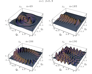
Figure 2: (Color online) Examples of wave functions in the plane $(Q_{1}\otimes Q_{2})$ for $\alpha=1$,$\beta=0.9$. Pronounced exotic states close to either displaced Fock states or “radial” states of the symmetric problem are shown. The extended (delocalized) state $n=190$ is shown for comparison.

For arbitrary $(\alpha,\beta)$ the Hamiltonian (1) can be exactly diagonalized in the electron subspace using the Fulton-Gouterman (FG) unitary operator Shore:1973

$$U=\frac{1}{\sqrt{2}}\left(\matrix{1\ ,\ R_{ph}\cr 1\ ,\ -R_{ph}}\right)$$ (3)

In the radial coordinates $\hat{Q}_{1}\rightarrow r\cos\phi$ and $\hat{Q}_{2}\rightarrow r\sin\phi$ the FG transformed Hamiltonian (1) for $p=+1$ is written as Majernikova:2005

$$\tilde{H}\equiv\hat{U}\hat{H}\hat{U}^{-1}=-\frac{1}{2r}\frac{\partial}{\partial r}\left(r\frac{\partial}{\partial r}\right)+\frac{1}{2}r^{2}-\frac{1}{2r^{2}}\frac{\partial^{2}}{\partial\phi^{2}}+$$

$$\sqrt{2}\alpha r\left(\cos\phi I-\sin\phi R_{ph}\sigma_{z}\right)+\sqrt{2}(\alpha-\beta)r\sin\phi R_{ph}\sigma_{z}$$ (4)

[here the reflection (2) acts as $R_{ph}(r,\phi)f(r,\phi)=f(r,\pi-\phi)$]. Investigation of E$\otimes$e case $\alpha=\beta$ in terms of rotational quantum numbers [eigenvalues of conserved angular momentum $\hat{J}=i(b_{1}b_{2}^{+}-b_{1}^{+}b_{2})-1/2\sigma_{y}$] has a long history, dating back to the paper in Long:1958 . The spectrum separates into irreducible representations, each characterizing by the quantum number $|j|=\frac{1}{2},\frac{3}{2},\dots$. The whole matrix is block-diagonal, and switching the term $\propto(\alpha-\beta)$ causes a complex interference of the levels in different blocks. The complicated structure of the energy levels is exemplified in Fig. 1 where we show 40 subsequent excited energy levels for $\alpha=2$ and varying $\beta$. The level avoidings are accompanied by level degeneracies (crossings). As in the symmetric case, there is a number of excited wave functions showing anomalous localization (Fig. 2) called ”exotic states” Wagner:1992 . One can recognize two distinct types of the ”exotic” states which are remnants of said limiting models with higher symmetry: in Fig.2 the state $n=185$ reminds us of the coherent state for $\beta=0$ while the states $n=69$ and $186$ with their markedly radial structure exemplify wave functions typical for the case $\alpha=\beta$.

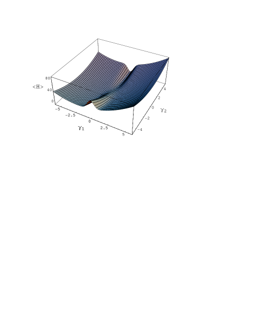
Figure 3: (Color online) Effective potential built on coherent states of both phonons. Its minima visualize complex interplay of effective quantum oscillators.

Far from the rotation symmetry it is more convenient to perform the transformation (3) in the space $\hat{Q}_{1}\times\hat{Q}_{2}$:

$$\tilde{H}_{FG}=\sum_{i=1,2}b_{i}^{{\dagger}}b_{i}+1+\alpha(b_{1}^{{\dagger}}+b_{1})-p\beta(b_{2}^{{\dagger}}+b_{2})R_{ph}\,.$$ (5)

The elimination of electron degrees of freedom reveals the nonlinearity hidden in the initial Hamiltonian (1) [terms with $R_{ph}$ in (4) or (5]. Hamiltonian (5) differs from that of exciton (dimer) by the phonon-2 assistance in the tunneling term $\beta(b_{2}^{{\dagger}}+b_{2})R_{ph}$ which accounts for Rabi oscillations by the virtual emission and absorption of the phonon-$1$. These oscillations are essentially the origin of the nonlinearity of the reflection symmetric model and of its quantum nature. Namely, a consecutively classical version of the model would require to set $R_{ph}\equiv\pm 1$ dropping the nonlinear term. Thus the equivalence between the models (1) and (5) is lost and the classical analog of the model (1) with $\beta\neq 0$ is self-controversial.

Averaging the diagonalized Hamiltonian (5) over the trial wave function chosen as a combination of coherent states $\exp[i\sum\limits_{k=1,2}R_{ph}(\gamma_{k}\hat{P}_{k}+\pi_{k}\hat{Q}_{k})]|0\rangle$ maps it onto a Husimi form Takahashi:1989 for two oscillators nonlinearly coupled in variables $\gamma_{i},\pi_{i}$. The “effective potential” (Husimi representation of the Hamiltonian operator) built on the coherent states in terms of the classical coordinates $\gamma_{1},\gamma_{2}$ (Fig. 3) was used for a variational treatment of the ground state problem Majernikova:2003 . We showed that the parameter space ($\alpha,\beta$) is separated onto two regions: the region $\alpha>\beta$ of the dominating self-trapping or ”heavy polaron” with large $\gamma_{1}\sim-\alpha$ and small $\gamma_{2}\sim\beta\exp(-2\gamma_{1}^{2})$ and that ($\alpha<\beta$) of the dominating tunneling between electron levels or ”light polaron” solution of small $\gamma_{1}$ and large $\gamma_{2}$. Quantum fluctuations cause mixing at the border between them and thus broaden the transition region. The potential in Fig. 3 visualizes the complex interplay of two oscillator potential wells resulting in the emerging of the third very narrow local minimum (at $\gamma_{1}\simeq 0$ and $\gamma_{2}>0$) responsible for the appearance of the light polaron (for more detailed discussion on this point see Majernikova:2002 ; Majernikova:2003 ). This heuristic visualization can be a guide for understanding phenomena in the excited spectrum as well. Excited states will follow the structure of either dominating self-trapping ($\alpha$) or tunneling ($\beta$) interactions.

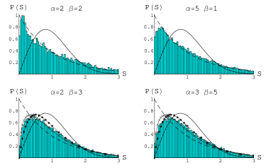
Figure 4: (Color online) Nearest-neighbor distributions of levels (unfolded and scaled to $\langle S\rangle=1$) for different values of $\alpha$, $\beta$. The curves on the histograms represent Poisson (long dashed), Wigner (full), semi-Poisson (stars) and $\sqrt{S}$ (crosses) distributions.

The level spacing distributions are considered as leading characteristics to distinguish between quantum integrability and chaos, the latter being described by the Wigner surmise (WD) $P_{W}(S)=(\pi/2)S\exp(-\pi S^{2}/4)$, and the former by the Poisson statistics (PD) $P_{P}(S)=\exp(-S)$ Gaspard:1990 ; Mehta:1960 ; Brody:1981 . Since long ago the Wigner surmise was conjectured as a limiting case for quantum chaotic behavior and supported from the point of view of random matrix theory (RMT; it is an exact conjecture for the 2$\times$2 RMT version, and a rather close approximation to the exactly solvable case of random matrices of infinite dimensions Mehta:1960 ). The PD is associated with the superposition of the multitude of uncorrelated levels: the falling exponential is a limiting case of a big number of independent level sequences, irrespectively to the level distributions inside each sequence Rosenzweig:60 . An adequate random-matrix model for our case of broken symmetry requires separately treating block and interblock elements Leitner:93 ; Leitner:94 yielding complicated statistical predictions as to the resulting superposition. Numerous interpolation formulas describing the intermediate situations between the complete integrability and chaos were considered Leitner:93 ; Brody:1981 . A simple interpolation based on the information theory considerations was suggested Robnik:87 in the form of the superposition of WD and PD: $P(S)\sim(\pi/2)S\exp(-\mu S-\nu S^{2})$. The accommodation constants $\mu$ and $\nu$ had to be chosen to ensure the normalization with $\langle S\rangle=1$ conditions and yielding some a priori given variance $\sigma^{2}$, thus giving a one-parameter interpolation because the variance monotonically changes from $(4/\pi-1)$ (WD) to $1$ (PD). Later on the theoretical background for this form of interpolation was enhanced on the base of the stochastic reformulation of the level statistics problem Hasegawa:88 . The semi-Poisson distribution (sPD) $P_{sP}(S)=4S\exp(-2S)$ with the dispersion exactly $0.5$ pertains to this class. Recently it was introduced to mimic new seemingly universal properties in certain classes of systems, in particular, being characteristics of the “critical quantum chaos” Evangelou:00 , therefore it is worthy to probe it as third reference point.

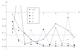
Figure 5: Standard deviations $\sigma^{2}=\langle S^{2}\rangle-1$ of the NNS distributions. Grid lines correspond to semi-Poisson (0.5) and $\sqrt{S}$ ($\frac{2}{3}$) values.

Figures 4 and 5 give the presentation of NNS statistics of JT system with varying $\alpha$ and $\beta$. The level spacings were unfolded according to the common procedure in order to exclude the secular changes of level density and to ensure $\langle S\rangle=1$. Figure 4 gives examples of NNS distributions for sample values of $\alpha$ and $\beta$. Figure 5 presents the standard deviations $\sigma^{2}\equiv\langle S^{2}\rangle-\langle S\rangle^{2}$ as functions of $(\alpha,\beta)$. In the vicinity of either $\alpha=\beta$, or $\alpha\gg\beta$, $\alpha\ll\beta$, the distribution functions $P(S)$ follow rather Poisson statistics (Fig. 4, first row), but small deviations of parameters from these cases abruptly bring the distributions away from it. Figure 5, however, reveals an interesting opposite universality for the parameters far from the one-parametric cases (that is supposedly in the most chaotic domain). The distribution functions seem to tend to a well-defined limit, but this limiting case does not resemble the Wigner surmise as one would expect. The standard deviation of all curves has lower boundary equal to $0.5$ (in Fig. 5 it is markedly seen for the curves corresponding to $\alpha\geq 2$ in the domains approximately $0.4\alpha\leq\beta\leq 2.5\alpha$ but apart from $\beta\simeq\alpha$). Note also in passing a remarkable mirror symmetry of interchange $\alpha\leftrightarrow\beta$: the corresponding level statistics are identical to a high degree of accuracy (the interchanged models however are not equivalent, and, for example, the wavefunctions of the ground state for $\alpha>\beta$ and $\alpha<\beta$ differ essentially Majernikova:2002 ; Majernikova:2003 ).

Thus, the concurrence of two phonon modes of the Hamiltonian and the existence of two symmetry-changing limits bring into being a new limiting distribution which can be considered as a ”most quantum chaotic” one for this system. We cannot conclude whether this hypothetic distribution is universal in the sense that it can encounter elsewhere. In the scope of the present paper we only try to mimic it discovering its possible universal properties. Natural suggestion is to compare it with the semi-Poisson distribution sharing the same $\sigma^{2}=0.5$ (Fig.4, second row). Quantitatively, a coefficient of deviation from universal limits of $P_{W}(S)$ and $P_{P}(S)$ can be introduced in the form Shklovskii:93 $\eta=\int_{0}^{S_{0}}[P(S)-P_{W}(S)]dS/\int_{0}^{S_{0}}[P_{P}(S)-P_{W}(S)]dS$ which gives the weight of the distribution left to the point $S_{0}\simeq 0.4729$ of the intersection of WD and PD and ranges from 0 (WD) to 1 (PD). For sPD $\eta_{sp}\simeq 0.3858$. The graphs of $\eta$ similar to that of Fig.5 again show the existence of a lower boundary $\eta\simeq 4.7>\eta_{sp}$. Hence, the sPD turns out to be much a better fit than WD, especially at $S\geq 1$. A systematic shift of the mass of the distribution to the left with respect to sPD is markedly observed in Fig.4. This shift is accounted for the nonlinear level repulsion of the actual distributions. At small $S\ll 1$ they scale as $P\sim S^{\delta}$. The actual repulsion index (Brody parameter) $\delta$ for ”chaotic sets” of $(\alpha,\beta)$ varies between $\sim 0.3$ and $0.5$, meanwhile the class of WD and sPD assumes a linear repulsion $P(S)\sim S$. Seeking for universal properties of a limiting distribution we use the maximum value $\delta=0.5$ and suggest another trial form $P_{sq}(S)\equiv(3\sqrt{3}/\sqrt{2\pi})\sqrt{S}\exp(-3S/2)$. The coefficient in the exponent is chosen to ensure $\langle S\rangle=1$ and to conform with the behavior of sPD at large $S$. Samples in Fig.4 (second row) show that $P_{sq}$-distribution reasonably fits actual distributions for small $S$ in the chaotic domain, although the latter have a tendency to shift slightly to the right. Therefore, the NNS distributions far from the $E\otimes e$ and Holstein limits appear to be confined between two suggested fitting formulas (note corresponding grid lines in Fig.5). The standard $\chi^{2}$ reliability test however shows significant deviations between actual distributions and both sPD and $P_{sq}$ indicating that neither of the reference distributions is a good fit in the strictly statistical sense.

The sPD was recently suggested to describe a narrow intermediate region between insulating and conducting regimes exemplified by the Anderson localization model Evangelou:00 , the mentioned opposite cases being described by correspondingly Poisson and Wigner statistics. At present a plausible analytical support (in the sense of RMT approaches) for this new distribution and for its universal character is lacking. It was found numerically Shklovskii:93 that the width of this intermediate domain strongly depends on the length $L$ of the system (its number of sites): for a system of infinite length one would get sPD in the narrow region of the Anderson parameter around $W_{cr}$, meanwhile for short lengths the width of the intermediate domain widens (in Shklovskii:93 the lengths of the order of $\simeq 5-10$ were checked). Jahn-Teller systems from this point of view can be considered as systems with $L=2$ (two electronic levels regarded as pseudo-sites); thus it is to expect that the ”transition domain” for such a system is rather large and plain in the parameter space, from whence there follows the applicability of sPD for almost all reasonable values of parameters $\alpha,\beta$. From the same point of view the systematic shift of the distribution to the left of sPD indicates that the generalized JT system is always closer to the ”insulator” phase meaning the dominance of ”heavy” polarons localized on one electronic level rather than the ”light” ones. It is not surprising since heavy polarons are associated with the broad well of the effective potential (Fig.3) which has a higher density of states than the narrow one responsible for light polarons. On the other hand, the empirically suggested second reference distribution is of Brody type Brody:1981 with the scaling $P\sim\sqrt{S}$ at small $S$. The Brody parameter can be related Meyer:1984 to the fraction of chaotic motion areas in the semiclassical picture. The present work gives merely a sketch of these possible relations, whose quantitative examination would be a challenge for the future study.

We acknowledge financial support from Project No. 202/06/0396 of the Grant Agency of the Czech Republic. Partial support is acknowledged from Project No. 2/6073/26 of the Grant Agency VEGA, Bratislava.

References

- (1) H. Eiermann and M. Wagner, J.Chem.Phys. 96, 4509 (1992).
- (2) A. Köngeter and M. Wagner, J.Chem.Phys. 92, 4003 (1990).
- (3) R. Graham M. Höhnerbach, Z. Phys. B: Condens.Matter 57, 233 (1984); Phys.Lett. 101A, 61 (1984).
- (4) J. Eidson and R. F. Fox, Phys. Rev. A 34, 3288 (1986); R. F. Fox and J. Eidson, Phys. Rev. A 34, 482 (1986); 36, 4321 (1987).
- (5) R. Blumel and B. Esser, Phys. Rev. Lett. 72, 3658 (1994); B. Esser and H. Schanz, Z. Phys. B:Condens. Matter 96, 553, (1995); H. Schanz and B. Esser, ibid. 101, 299 (1996); H. Schanz and B. Esser, Phys. Rev. A 55, 3375 (1997).
- (6) M. Sonnek et al., Phys. Rev. B 49, 15637 (1994).
- (7) U. Herfort and M. Wagner, J. Phys.: Condens. Matter 13, 3297 (2001).
- (8) B. Eckhardt, Phys. Rep. 163, 205 (1988).
- (9) K. Nakamura, Quantum Chaos – A New Paradigm of Nonlinear Dynamics (Cambridge University Press, Cambridge, 1993).
- (10) T. A. Brody et al., Rev. Mod. Phys. 53, 385 (1981).
- (11) H. B. Shore and L. M. Sander, Phys. Rev. B 7, 4537 (1973).
- (12) E. Majerníková et al., Phys. Rev. B 65, 174305 (2002).
- (13) Y. E. Perlin and M. Wagner, in The Dynamical Jahn-Teller Effect in Localized Systems, edited by Y. Perlin and M. Wagner (Elsevier Science Publishers, New York, 1984), p.1.
- (14) E. Majerníková and S. Shpyrko, J. Phys.: Condens. Matter 15, 2137 (2003).
- (15) H. Yamasaki et al., Phys. Rev. E 68, 046201 (2003).
- (16) M. C. M. O’Brien, Proc. Roy. Soc. London,Ser.A A281, 323 (1964).
- (17) E. Majerníková and S. Shpyrko, Phys. Rev. E 73 No 6 (in press); cond-mat/0509687.
- (18) H. C. Longuet-Higgins et al., Proc. Roy. Soc. London, Ser.A A244, 1 (1958).
- (19) K. Takahashi, Prog. Theor. Phys. Suppl, 98, 109 (1989).
- (20) M.L.Mehta, Nucl.Phys. 18, 395 (1960); M. L. Mehta and M. Gaudin, ibid. 18, 420 (1960); M. Gaudin, ibid. 25, 447 (1961).
- (21) P. Gaspard et al., Phys. Rev. A 42, 4015 (1990).
- (22) N. Rosenzweig and C. E. Porter, Phys. Rev. 120, 1968 (1960).
- (23) D. M. Leitner, Phys. Rev. E 48, 2536 (1993).
- (24) D. M. Leitner et al., Phys. Rev. Lett. 73, 2970 (1994); E. Haller et al., Phys. Rev. Lett. 52, 1665 (1984).
- (25) M. Robnik, J.Phys.A 20, L495 (1987).
- (26) H. Hasegawa et al., Phys. Rev. A 38, 395 (1988).
- (27) S. N. Evangelou and J.-L. Pichard, Phys. Rev. Lett. 84, 1643 (2000); S. N. Evangelou and D. E. Katsanos, Phys. Lett. A334, 331 (2005); E. B. Bogomolny et al., Phys. Rev. E 59, R1315 (1999).
- (28) B. I. Shklovskii et al., Phys. Rev. B 47, 11487 (1993).
- (29) H.-D. Meyer et al., J. Phys. A 17, L831 (1984); A. Shudo, Prog. Theor. Phys. Suppl. 98, 173 (1989).