Soliton ratchets in homogeneous nonlinear Klein-Gordon systems

Abstract

We study in detail the ratchet-like dynamics of topological solitons in homogeneous nonlinear Klein-Gordon systems driven by a bi-harmonic force. By using a collective coordinate approach with two degrees of freedom, namely the center of the soliton, $X(t)$, and its width, $l(t)$, we show, first, that energy is inhomogeneously pumped into the system, generating as result a directed motion; and, second, that the breaking of the time shift symmetry gives rise to a resonance mechanism that takes place whenever the width $l(t)$ oscillates with at least one frequency of the external ac force. In addition, we show that for the appearance of soliton ratchets, it is also neccesary to break the time-reversal symmetry. We analyze in detail the effects of dissipation in the system, calculating the average velocity of the soliton as a function of the ac force and the damping. We find current reversal phenomena depending on the parameter choice and discuss the important role played by the phases of the ac force. Our analytical calculations are confirmed by numerical simulations of the full partial differential equations of the sine-Gordon and $\phi^{4}$ systems, which are seen to exhibit the same qualitative behavior. Our results show features similar to those obtained in recent experimental work on dissipation induced symmetry breaking.

LEAD PARAGRAPH

Ratchet, or rectification, phenomena in nonlinear nonequilibrium systems are receiving a great deal of attention in the past few years. A typical example of a ratchet occurs when point-like particles are driven by deterministic or non-white stochastic forces: Under certain conditions related to the breaking of symmetries, unidirectional motion can take place although the applied force has zero average in time. The broken symmetries can be spatial, by introducing an asymmetric potential, or temporal, by using asymmetric periodic forces. This effect has found many applications in the design of devices for rectification or separation of different particles. Recently, ratchet dynamics is being studied in the context of solitons, trying to understand whether the fact that solitons, or nonlinear coherent excitations in general, are extended objects, allows for similar rectification phenomena. In nonlinear Klein-Gordon systems, it has been shown that ratchet-like behavior can be observed when driven by asymmetric periodic forces. However, the phenomenon is different from that seen in point-like particles as the deformations of the soliton play a crucial role. In this paper we describe in detail these phenomena, analyze the mathematical conditions for its existence, explain the underlying mechanism originating the net motion, and study the highly non-trivial effects of dissipation on the motion. Our results may be related to recent observations of rectification in Josephson junctions and optical lattices.

I Introduction

Ratchet or rectification phenomena, the subject of an intense research effort during the last decade, appear in very many different fields ranging from nanodevices to molecular biology Hanggi1 ; Astumian ; Ajdari ; Reimann ; Linke ; Hanggi2 ; doering . Generally speaking, the appearance of ratchet-like behavior requires two ingredients: Departure from thermal equilibrium, either by using correlated stochastic forces or deterministic forces, and breaking of spatial and/or temporal symmetries Reimann ; Hanggi2 ; asym ; save ; Borromeo ; Marchesoni ; maskk ; Morales . Many applications of the ratchet theoretical framework deal with the scenario of spatial symmetry breaking, beginning with the proposal for nonequilibrium rectifiers in Hanggi1 . However, in other problems, breaking the temporal symmetry may be much more feasible; this is the case, for instance, of optical lattices schia or Josephson junctions Zapata ; JJ1 ; JJ2 (see also kk for related work on Josephson ratchets in the dissipative quantum regime) when driven by an appropriate bi-harmonic force. In this context, the ratio of the frequencies of a bi-harmonic force is related with the breaking of the temporal-shift symmetry, (given by $f(t)=-f(t+T/2)$ with $T$ being the period) whereas suitable choices for the driving phases and damping optical2 lead to time-reversal symmetry breaking ricardo . This mechanism to obtain directed motion from a zero-mean force has been first proposed for particle (zero-dimensional) systems Reimann ; asym ; referee-flach , and it has recently been extended to extended systems, both classical flach ; Salerno-mixing ; Marchesoni ; maskk and quantum ones Goychuk .

A very relevant system, mostly because its character of paradigmatic of phenomena arising in connection with topological solitons and its many applications, is the damped and driven sine-Gordon (sG) model Scott :

$$\phi_{tt}-\phi_{xx}+\sin(\phi)=-\beta\phi_{t}+f(t).$$ (1)

In Salerno-mixing the symmetry considerations above were studied in the context of Eq. (1) by choosing

$$f(t)=\epsilon_{1}\sin(\delta t+\delta_{0})+\epsilon_{2}\sin(m\delta t+\delta_{0}+\theta^{\prime})=\epsilon_{1}\sin(\delta t+\theta_{1})+\epsilon_{2}\sin(m\delta t+\theta_{2}),$$ (2)

where $m$ is an integer number and $\epsilon_{1}$ ($\epsilon_{2}$) is the amplitude of the harmonic component with frequency $\delta$ ($m\delta$) and phase $\theta_{1}$ ($\theta_{2}$). We note that in the equation above $\theta_{1}=\delta_{0}$ y $\theta^{\prime}=\theta_{2}-\theta_{1}$, being $\theta^{\prime}$ the relative phase, and therefore the results presented here can be understood as well in terms of relative phases. The reason for including two harmonics is that, as can be seen immediately from the previous symmetry analysis, in the case of a single harmonic the directed motion of sG kinks is not possible, something advanced by a different reasoning some years ago niurka5 and experimentally confirmed in goldo . Thus, the main result in Salerno-mixing was the finding that, if $f(t)$ breaks the shift symmetry and if the total topological charge in the system is nonzero, a directed current (meaning a preferential motion of the kink in one direction) could be observed whose direction and magnitude depend on the driving parameters and damping coefficient.

Subsequently, in a recent paper morales , we advanced a first explanation of the mechanisms underlying the observations in Salerno-mixing : Directed motion of solitons arises because of a resonance phenomenon involving the oscillations of the soliton width, $l(t)$, with at least one of the frequencies of the ac force. In terms of the symmetry picture we are discussing here, we note that it is precisely the breaking of the shift symmetry the reason for the appearance of the resonance, which means that the shift symmetry and the resonance conditions are equivalent. In the present work we will extend our preliminary results in morales in several directions. First, we will show that net motion of the soliton is only possible if, in addition to the aforementioned resonance condition on the frequencies, the time-reversal symmetry is also broken by the action of ac force and damping. As will be seen below, this in turn implies that the energy introduced by the biharmonic force is inhomogeneously pumped into the system, giving rise to the observed unidirectional motion. Second, we will carry out a detailed study of the ratchet dynamics of solitons governed by Eq. (1), including not only the cases $m=2$, our main focus in morales , but also $m=4$, which we compare to the previous one. Third, in order to show the generality of our results, we will present an analysis of the motion of the $\phi^{4}$ kink, whose dynamics is given by

$$\phi_{tt}-\phi_{xx}+\phi^{3}-\phi=-\beta\phi_{t}+f(t).$$ (3)

Finally, we will extend our previous work to analyze in depth the influence of dissipation in the directional motion. We will focus on the way that damping affects the phase values for which there is no soliton motion, and we will discuss the existence of values of the dissipation coefficient that lead to optimal soliton mobility. Interestingly, our results are reminiscent of the experimental findings in optical2 , where similar effects due to dissipation are found.

The presentation of the above results is organized as follows: In the next Section we analyze twp nonlinear Klein-Gordon systems, specifically the sine-Gordon and $\phi^{4}$ models, by means of a collective coordinate (CC) approach, obtaining the analytical and approximate expressions for the average of the velocity of the center of the soliton for $m=2$ and $m=4$. In Section III we verify our analytical results by means of numerical simulations. Section IV is devoted to the discussion of the most relevant effects of dissipation. To conclude the paper, in the last section we recapitulate the results of Sections III–V, make the connection with the experiments and summarize our main findings.

II Collective coordinate approach

II.1 Collective coordinate equations

Our aim in this section is to obtain an approximate expression for the average velocity of the center of the kink (as $\phi^{4}$ kinks are not solitons, strictly speaking, we will refer to these excitations of both models as kink from now on). To this end, we will use one of the different CC approaches (see siam for a review). We introduce two variables, namely the center of the kink, $X(t)$, and its width, $l(t)$, through Rice’s Ansatz rice , which amounts to specifying the kink solution as

$$\phi_{0}(x,t)=4\,{\rm arctan}\left[\exp\left(\frac{x-X(t)}{l(t)}\right)\right],$$ (4)

for sG and

$$\phi_{0}(x,t)=\tanh\left[\frac{x-X(t)}{l(t)}\right],$$ (5)

for $\phi^{4}$. Using the above expressions, and the variations of the energy and the momentum (two conserved quantities of the unperturbed systems Eqs. (1) and (3)) it can be shown (see niurka2 for details) that the two collective variables obey the following two ordinary differential equations:

$$\frac{dP}{dt}=-\beta P-qf(t),$$ (6)

$$\dot{l}^{2}-2l\ddot{l}-2\beta l\dot{l}=\Omega_{R}^{2}l^{2}\left[1+\frac{P^{2}}{M_{0}^{2}}\right]-\frac{1}{\alpha},$$ (7)

where $P(t)\equiv M_{0}l_{0}\dot{X}/l(t)$, $\Omega_{R}=1/(\sqrt{\alpha}l_{0})$ is Rice’s frequency, and the parameters $M_{0}$, $q$, $\alpha$ and $l_{0}$ take different values according to the model, sG or $\phi^{4}$ (see Table 1).

Parameters	sine-Gordon	$\phi^{4}$
$q$	$2\pi$	$2$
$M_{0}$	$8$	$2\sqrt{2}/3$
$l_{0}$	$1$	$\sqrt{2}$
$\alpha$	$\pi^{2}/12$	$(\pi^{2}-6)/12$

Table 1: Parameters corresponding to the two nonlinear Klein-Gordon models we work with, the sine-Gordon and $\phi^{4}$ models. $q$ is the topological charge, $M_{0}$ and $l_{0}$ are the mass and the width of the kink at rest.

The quantity $P(t)$ deserves some discussion on in its own. To begin with, it represents the momentum of the kink: Indeed, the expression for $P(t)$ can be obtained as well by substituting Rice’s Ansatz into the definition of the momentum $P(t)=-\textstyle\int_{-\infty}^{+\infty}dx\,\ \phi_{t}\phi_{x}$. The same equations can be obtained using a projection technique with a Generalized Traveling Wave Ansatz (GTWA) (see details in niurka3 ). In addition, it has been shown recently comment that Eq. (6) for the momentum, obtained here within the framework of the Rice approximation, is an exact equation of motion, irrespective of the choice for the Ansatz. Hence, its solution is also exact and not an approximation.

Let us now proceed with the analysis of Eqs. (6) and (7). After transients have elapsed and become negligible, ($t\gg 1/\beta$) the solution for $P(t)$ is essentially given by

$$\ P(t)=-\sqrt{\epsilon}[a_{1}\sin(\delta t+\theta_{1}-\chi_{1})+a_{2}\sin(m\delta t+\theta_{2}-\chi_{m})],$$ (8)

where $\epsilon\equiv\displaystyle\mbox{min}(\epsilon_{1},\epsilon_{2})$ is a rescaling parameter, and

$$\displaystyle\chi_{1} = \arctan\left(\frac{\delta}{\beta}\right),\quad\chi_{m}=\arctan\left(\frac{m\delta}{\beta}\right),$$ (9)

$$\displaystyle a_{1} = \frac{q}{\sqrt{\beta^{2}+\delta^{2}}}\frac{\epsilon_{1}}{\sqrt{\epsilon}},\quad{\rm and}\quad\displaystyle a_{2}=\frac{q}{\sqrt{\beta^{2}+m^{2}\delta^{2}}}\frac{\epsilon_{2}}{\sqrt{\epsilon}}.$$ (10)

We can now turn to Eq. (7), which is nothing but a parametrically driven oscillator: it is clear that $l(t)$ is indirectly driven by the harmonic forces with frequencies $\delta$ and $m\,\delta$, due to the term $P^{2}$ on the r.h.s of Eq. (7). To solve (approximately) this equation, we expand $l(t)$ in powers of $\epsilon$ around the unperturbed kink width $l_{0}$:

$$l(t)=l_{0}+\epsilon l_{1}(t)+\epsilon^{2}l_{2}(t)+...\,\,\ .$$ (11)

Substituting Eq. (11) into Eq. (7) we find a hierarchy of equations for different orders of powers in $\epsilon$. The first three equations for $l_{i}(t)$ are given by:

$$\ddot{l}_{1}(t)+\beta\dot{l}_{1}(t)+\Omega_{R}^{2}l_{1}(t) = -\frac{\Omega_{R}^{2}}{2\epsilon M_{0}^{2}}P^{2}(t)l_{0},$$ (12)

$$\ddot{l}_{2}(t)+\beta\dot{l}_{2}(t)+\Omega_{R}^{2}l_{2}(t) = -\frac{\Omega_{R}^{2}}{2\epsilon M_{0}^{2}}P^{2}(t)l_{1}+\frac{\dot{l}_{1}^{2}}{2l_{0}}+\frac{\Omega_{R}^{2}l_{1}^{2}}{2l_{0}}$$ (13)

$$\ddot{l}_{3}(t)+\beta\dot{l}_{3}(t)+\Omega_{R}^{2}l_{3}(t) = -\frac{\Omega_{R}^{2}}{2\epsilon M_{0}^{2}}P^{2}(t)l_{2}+\frac{\dot{l}_{1}\dot{l}_{2}}{l_{0}}+\frac{\Omega_{R}^{2}l_{1}l_{2}}{l_{0}}-\frac{\dot{l}_{1}^{2}l_{1}}{2l_{0}^{2}}-\frac{\Omega_{R}^{2}l_{1}^{3}}{2l_{0}^{2}}.$$ (14)

These equations are linear and therefore we can begin by solving the first one, Eq. (12), by substituting the expression for the momentum, Eq. (8), into the r.h.s of (12). With this, the equation for $l_{1}$ becomes

$$\ddot{l}_{1}(t)+\beta\dot{l}_{1}(t)\Omega_{R}^{2}l_{1}(t) = A_{1}+A_{2}\cos(2\delta t+2\theta_{1}-2\chi_{1})+A_{3}\cos(2m\delta t+2\theta_{2}-2\chi_{m})+$$ (15)

$$+ A_{4}\Big{\{}\cos[(m-1)\delta t+\theta_{2}-\theta_{1}-(\chi_{m}-\chi_{1})]-\cos[(m+1)\delta t+\theta_{1}+\theta_{2}-(\chi_{m}+\chi_{1})]\Big{\}},$$

where

$$A_{1} = -A_{2}-A_{3},$$ (16)

$$A_{2} = \frac{\Omega_{R}a_{1}^{2}}{4\sqrt{\alpha}M_{0}^{2}},$$ (17)

$$A_{3} = \frac{\Omega_{R}a_{2}^{2}}{4\sqrt{\alpha}M_{0}^{2}},$$ (18)

$$A_{4} = -\frac{\Omega_{R}}{2\sqrt{\alpha}M_{0}^{2}}a_{1}a_{2}.$$ (19)

It is important to notice on the r.h.s of Eq. (15) the presence of harmonics with frequencies $2\delta$, $2m\delta$ and $(m\pm 1)\delta$. As a consequence, all these frequencies appear in the expression for $l_{1}(t)$ and they remain after a transient time $t\gg 1/\beta$, i.e., asymptotically we have

$$l_{1}(t)= \frac{A_{1}}{\Omega_{R}^{2}}+\frac{A_{2}\sin(2\delta t+2\theta_{1}-2\chi_{1}+\tilde{\theta}_{2})}{\sqrt{(\Omega_{R}^{2}-4\delta^{2})^{2}+4\beta^{2}\delta^{2}}}+\frac{A_{3}\sin(2m\delta t+2\theta_{2}-2\chi_{m}+\tilde{\theta}_{2m})}{\sqrt{(\Omega_{R}^{2}-4m^{2}\delta^{2})^{2}+4m^{2}\beta^{2}\delta^{2}}}$$ (20)

$$+\frac{A_{4}\sin[(m-1)\delta t+\theta_{2}-\theta_{1}-(\chi_{m}-\chi_{1})+\tilde{\theta}_{m-1}]}{\sqrt{(\Omega_{R}^{2}-(m-1)^{2}\delta^{2})^{2}+\beta^{2}(m-1)^{2}\delta^{2}}}$$

$$-\frac{A_{4}\sin[(m+1)\delta t+\theta_{1}+\theta_{2}-(\chi_{m}+\chi_{1})+\tilde{\theta}_{m+1}]}{\sqrt{(\Omega_{R}^{2}-(m+1)^{2}\delta^{2})^{2}+\beta^{2}(m+1)^{2}\delta^{2}}},$$

where

$$\tilde{\theta}_{m}=\arctan\left(\frac{\Omega_{R}^{2}-m^{2}\delta^{2}}{m\beta\delta}\right).$$

From the r.h.s of Eqs. (13) and (14), the same reasoning as above leads one to find the harmonics corresponding to the second and third order corrections $l_{2}(t)$ and $l_{3}(t)$. We do not include the explicit expressions for these corrections for the sake of brevity, but in Table 2 we collect all these values for $m=2,3,4$.

$2^{nd}$ harmonic($\delta$)	$l_{1}$	$l_{2}$
m	$2\delta$, $2m\delta$, $(m\pm 1)\delta$	$2\delta$, $4\delta$, $4m\delta$, $(m\pm 1)\delta$,
		$2(m\pm 1)\delta$, $(m\pm 3)\delta$, $(3m\pm 1)\delta$
2	$\delta$, $2\delta$, $3\delta$, $4\delta$	$\delta$, $2\delta$, $3\delta$, $4\delta$, $5\delta$, $6\delta$, $7\delta$, $8\delta$
3	$2\delta$, $4\delta$, $6\delta$	$2\delta$, $4\delta$, $6\delta$, $8\delta$, $10\delta$, $12\delta$
4	$2\delta$, $3\delta$, $5\delta$, $8\delta$	$\delta$, $2\delta$, $3\delta$, $4\delta$, $5\delta$, $7\delta$,
		$9\delta$, $10\delta$, $11\delta$, $13\delta$, $16\delta$

Table 2: Harmonic content of the first contributions to the perturbative expansion of $l(t)$. Notice that $\delta$ and $m\delta$ are the frequencies of the ac force (they appear in the momentum equation as well).

II.2 Velocity of the kink center

Having found the exact expression for $P(t)$ and the first terms in the perturbative expansion for $l(t)$, we can now calculate the average velocity over one period $T=2\pi/\delta$. To this end, we recall the previously defined expression for the momentum, $P(t)=M_{0}l_{0}\dot{X}/l(t)$. After transients have elapsed, which means after a time essentially given by the inverse of the dissipation coefficient, the mean velocity of the kink can be expressed in terms of the CC as

$$\langle\dot{X}(t)\rangle=\frac{1}{T}\int_{0}^{T}\frac{P(t)l(t)}{M_{0}l_{0}}dt.$$ (21)

Taking into account the expansion (11), this expression can be written as

$$\langle\dot{X}(t)\rangle = \frac{1}{T}\int_{0}^{T}\frac{P(t)(l_{0}+\epsilon l_{1}(t)+\epsilon^{2}l_{2}(t)+...)}{M_{0}l_{0}}dt$$ (22)

$$= \langle\dot{X}_{0}(t)\rangle+\epsilon\langle\dot{X}_{1}(t)\rangle+\epsilon^{2}\langle\dot{X}_{2}(t)\rangle+...$$

Therefore, as already stated, the mean velocity can be analytically (and approximately) calculated taking into account the exact solution for the momentum (8) and the first terms of the expansion for the width of the kink. At order $O(\epsilon^{0})$, $\langle\dot{X}_{0}(t)\rangle\sim\langle P(t)\rangle=0$ since the average of the momentum is zero [see Eq. (8)]. Accordingly, the net motion of the kink can only arise from the contribution of higher order terms; hence, we proceed by computing the integral defining $\epsilon\langle\dot{X}_{1}(t)\rangle$. Inserting Eqs. (8) and (20) in (22), straightforward calculations show for $m=2$ that

$$\epsilon\langle\dot{X}_{1}\rangle = \frac{q^{3}\Omega_{R}^{2}\epsilon_{1}^{2}\epsilon_{2}}{8M_{0}^{3}(\beta^{2}+\delta^{2})\sqrt{\beta^{2}+4\delta^{2}}}\left(\frac{2\cos[2\theta_{1}-\theta_{2}+(\chi_{2}-2\chi_{1})-\tilde{\theta}_{1}]}{\sqrt{(\Omega_{R}^{2}-\delta^{2})^{2}+\beta^{2}\delta^{2}}}\right.$$ (23)

$$\left.-\frac{\cos[2\theta_{1}-\theta_{2}+(\chi_{2}-2\chi_{1})+\tilde{\theta}_{2}]}{\sqrt{(\Omega_{R}^{2}-4\delta^{2})^{2}+4\beta^{2}\delta^{2}}}\right).$$

It is important to recall that for the CC approach to be valid, we must require that the kink shape is not very much distorted, and hence that $\epsilon_{i}\ll 1$ and $\delta\ll 1$. Moreover, we would like to stress that expression (23) is valid only for any finite but nonzero value of $\beta$, since we have obtained it for $t>>1/\beta$.

We can recast Eq. (23) in a simpler form to make more transparent the dependencies on the different parameters, as follows:

$$\epsilon\langle\dot{X}_{1}\rangle = \epsilon_{1}^{2}\,\epsilon_{2}\,\Gamma_{1}(\beta,\delta)\sin[\theta_{2}-2\theta_{1}+\Phi_{1}(\beta,\delta)],$$ (24)

where we have introduced an amplitude, $\Gamma_{1}$, whose specific form is not needed and is therefore omitted for brevity, and a phase,

$$\Phi_{1}(\beta,\delta)=2\chi_{1}-\chi_{2}-\arctan\left[\frac{2\beta\delta[(\Omega_{R}^{2}-4\delta^{2})^{2}+3\beta^{2}\delta^{2}-(\Omega_{R}^{2}-\delta^{2})^{2}]}{2(\Omega_{R}^{2}-\delta^{2})[(\Omega_{R}^{2}-4\delta^{2})^{2}+4\beta^{2}\delta^{2}]+(\Omega_{R}^{2}-4\delta^{2})[(\Omega_{R}^{2}-\delta^{2})^{2}+\beta^{2}\delta^{2}]}\right],$$ (25)

which are only functions of the dissipation coefficient and the frequencies of the ac force. We note here that a similar expression, albeit starting from a less general Ansatz, has been obtained in Salerno-mixing . In this new form, it is apparent that the averaged velocity is a sinusoidal function of $\theta_{1}$ and $\theta_{2}$, and it is proporcional to $\epsilon_{1}^{2}\,\epsilon_{2}$. It is interesting to note that the same dependence on amplitudes and phases is also found in other systems, in principle unrelated with the ratchet dynamics of solitons we are discussing here (see ricardo and references therein). On the other hand, from the experimental viewpoint, it is worth noting that, in the limit $\delta\ll\beta$, we find $\langle V\rangle\sim\sin(2\theta_{1}-\theta_{2})$, in agreement with the experiments on JJ reported in JJ2 .

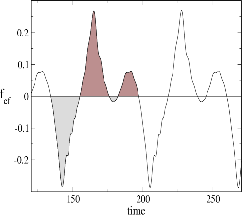
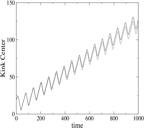
Figure 1: a) Effective driving force in the sG model as a function of time. b) Trajectory of the center of the soliton; dashed line: CC result obtained by numerically integrating Eqs. (6) and (7); solid line: simulations of the full sG equation. Parameters used in both figures are $\delta=0.1$, $m=2$, $\beta=0.05$, $\theta_{2}=-2.5$, $\theta_{1}=0$, $\epsilon_{1}=\epsilon_{2}=0.2.$

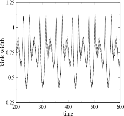
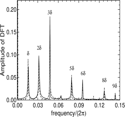
Figure 2: Ratchet dynamics in the sG model for $m=2$. Left panel: Width of the kink vs time. Right panel: Discrete Fourier Transform (DFT) of the width of the kink. In both panels the dashed lines represent the numerical solution of Eqs. (6-7) and the solid lines the computed width from the numerical simulation of Eq. (1). Parameters are $\epsilon_{1}=\epsilon_{2}=0.2$, $\beta=0.05$, $\delta=0.1$, $\theta_{1}=-2.5$ $\theta_{2}=\pi/2-2.5$.

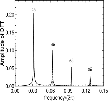
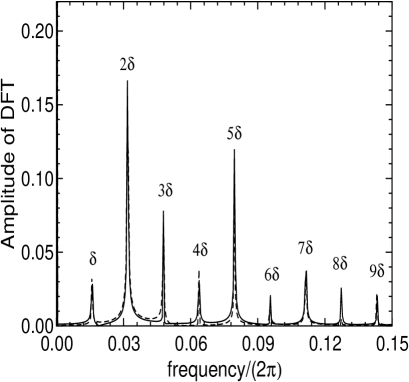
Figure 3: Discrete Fourier Transform of the kink width. Left panel: $m=3$ (no net motion); Right panel: $m=4$ (ratchet motion of the kink takes place). Solid line: amplitude measured in simulations. Dashed line: amplitude as obtained by numerical integration of the CC equations (6)-(7). The parameters of the ac force and the dissipation coefficient are the same as in Fig. 2.

Proceeding with the analysis of the average velocity of the kink, from Eq. (24) it is obvious that net motion (i.e., with nonzero average velocity) is only possible if

$$2\theta_{1}-\theta_{2}-\Phi_{1}\neq n\pi,n=0,1,...$$ (26)

In this form, this condition, as will be shown below (and was pointed out in optical2 ), arises from the breaking of the time-reversal symmetry by the biharmonic force. Indeed, $\Phi_{1}$ is related with the difference of phases between the harmonics with frequencies $\delta$ and $m\delta$ in the functions $P(t)$ and $l_{1}(t)$. Thus, our first resonance criterion reads that the ratchet effect appears when $l(t)$ oscillates with at least one of the frequencies of $P(t)$; in addition, the difference of phases between the harmonics must be appropriate for the appeareance of net motion. In others words, fixing all the parameters of the ac force and damping except one of the two phases of the ac force, one can find a critical value of that phase that suppresses directed motion of kinks. The values at which the velocity vanishes are important, since for a force with a given frequency and damping, they indicate the phases at which the velocity of the kink is reversed. On the other hand, the changes in the phases are related with the breaking of the time-reversal symmetry of the system denisov .

Let us now turn to the case $m=4$, a value for which the appearance of the ratchet effect is also predicted Salerno-mixing . In analogous manner to the preceding calculations, one can show that $\epsilon\langle\dot{X}_{1}\rangle$ is zero. Therefore, the frequencies in $l(t)$ that contribute to the net motion must appear in higher order corrections (see Table 2), namely $\epsilon^{2}\langle\dot{X}_{2}\rangle$. After cumbersome calculations we find

$$\epsilon^{2}\langle\dot{X}_{2}\rangle = \frac{q^{5}\Omega_{R}^{4}\epsilon_{1}^{4}\epsilon_{2}}{32M_{0}^{5}(\beta^{2}+\delta^{2})^{2}\sqrt{(}\beta^{2}+16\delta^{2})}\,\ \mbox{x}$$ (27)

$$\left\{\frac{\sin(4\theta_{1}-\theta_{2}+\chi_{4}-4\chi_{1}+\tilde{\theta}_{2}-\tilde{\theta}_{1})}{\sqrt{(\Omega_{R}^{2}-\delta^{2})^{2}+\beta^{2}\delta^{2}}\sqrt{(\Omega_{R}^{2}-4\delta^{2})^{2}+4\beta^{2}\delta^{2}}}\right.$$

$$\left.+\frac{(6\delta^{2}+\Omega_{R}^{2})\cos(4\theta_{1}-\theta_{2}+\chi_{4}-4\chi_{1}-\tilde{\theta}_{3}+\tilde{\theta}_{2}-\tilde{\theta}_{1})}{\sqrt{(\Omega_{R}^{2}-\delta^{2})^{2}+\beta^{2}\delta^{2}}\sqrt{(\Omega_{R}^{2}-4\delta^{2})^{2}+4\beta^{2}\delta^{2}}\sqrt{(\Omega_{R}^{2}-9\delta^{2})^{2}+9\beta^{2}\delta^{2}}}\right.$$

$$\left.-\frac{\sin(4\theta_{1}-\theta_{2}+\chi_{4}-4\chi_{1}-\tilde{\theta}_{3}-\tilde{\theta}_{1})}{\sqrt{(\Omega_{R}^{2}-\delta^{2})^{2}+\beta^{2}\delta^{2}}\sqrt{(\Omega_{R}^{2}-9\delta^{2})^{2}+9\beta^{2}\delta^{2}}}\right.$$

$$\left.-\frac{\sin(4\theta_{1}-\theta_{2}+\chi_{4}-4\chi_{1}+\tilde{\theta}_{2}+\tilde{\theta}_{4})}{2\sqrt{(\Omega_{R}^{2}-4\delta^{2})^{2}+4\beta^{2}\delta^{2}}\sqrt{(\Omega_{R}^{2}-16\delta^{2})^{2}+16\beta^{2}\delta^{2}}}\right.$$

$$-\frac{(4\delta^{2}-\Omega_{R}^{2})\cos(4\theta_{1}-\theta_{2}+\chi_{4}-4\chi_{1}+2\tilde{\theta}_{2}+\tilde{\theta}_{4})}{4[(\Omega_{R}^{2}-4\delta^{2})^{2}+4\beta^{2}\delta^{2}]\sqrt{(\Omega_{R}^{2}-16\delta^{2})^{2}+16\beta^{2}\delta^{2}}}\Bigg{\}},$$

which can be rewritten as

$$\epsilon^{2}\langle\dot{X}_{2}\rangle = \epsilon_{1}^{4}\epsilon_{2}\Gamma_{2}(\beta,\delta)\sin[\theta_{2}-4\theta_{1}+\Phi_{2}(\beta,\delta)],$$ (28)

where again the amplitude, $\Gamma_{2}$, and the phase, $\Phi_{2}$, are functions of the dissipation and the frequencies of the ac force. As for the mobility condition, which for the $m=2$ case was given by Eq. (26), a similar expression can be derived for the case $m=4$ by imposing that the sine function vanishes in Eq. (28).

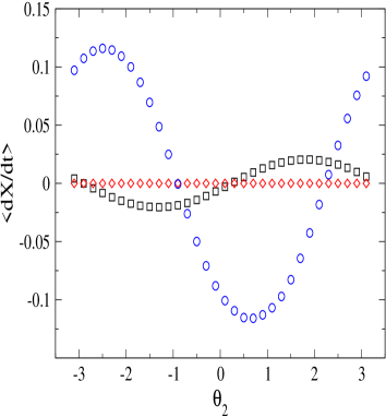
Figure 4: Dependence of the average velocity of a sG kink on the phase, $\theta_{2}$, for different values of $m$. $m=2$ (blue circles); $m=3$ (red diamonds) and $m=4$ (black squares). Parameters are $\epsilon_{1}=\epsilon_{2}=0.2$, $\beta=0.05$, $\delta=0.1$, $\theta_{1}=0$.

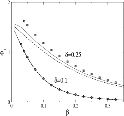
Figure 5: Dependence of the function $\Phi_{1}=-\theta_{2}^{c}$ on the dissipation coefficient for $m=2$ and $\beta\geq 0.01$. In the simulations as well as in the CC, we find $\theta_{2}^{c}$ as the value of the phase between $-\pi$ and 0 for which the motion is suppressed. Solid line: CC result; dashed line: Eq. (25); symbols: numerical simulations of the full sine-Gordon equation. Parameters are $\epsilon_{1}=\epsilon_{2}=0.2$ and $\theta_{1}=0$.

For the case $m=3$, the shift-symmetry is not broken and therefore ratchet motion can not take place. Indeed, the calculation of the average velocity based on the CC approach gives zero for all orders of the expansion. For this case the frequencies of the ac force (or the momentum) are odd harmonics of $\delta$ ($\delta$ and $3\delta$), whereas only even harmonics of $\delta$ are found in the kink width oscillations ($2n\delta$, $n\in N$). The complete selection rules for $m=2,3,4$ appear in Table 2, where for a given $m$ one identifies the harmonics corresponding to the oscillations of the width of the kink. Resonances take then place when at least one of these harmonics coincides with one of the two harmonics of the ac force. We can verify that if this condition is fullfiled, the shift symmetry is broken and viceversa. In the simplest case, $m=1$, for which the driving consists only of a single harmonic, the ratchet effect is also absent. Looking at Eq. (8) it is immediately realized that only terms with frequency $2\delta$ appear in the equation (7), so that the resonance condition is not achieved in agreement with previous results niurka2 . This discussion in terms of resonant frequencies can be extended, in an analogous but cumbersome calculation, to any positive integer number of the frequency of the second harmonic, i.e., for higher integer values of $m$. Finally, an interesting remark is that the resonance condition can also be interpreted as a synchronization between the ac force and the oscillations of the width of the kink, i.e., directional transport occurs whenever the ac force is locked to the oscillations of the width salerno2 .

II.3 Mechanism for directional motion

In the previous subsection we have established the conditions for net motion of the kink to take place. We argued that the fact that the width of the kink is a dynamical variable is not a sufficient condition for the existence of directed motion and, on the contrary, net motion can arise only when, first, at least one of the two harmonics of the ac driven force appears in the oscillations of the width of the kink (which is equivalent to breaking the shift symmetry) and, second, when the time-reversal symmetry is broken. However, these two conditions, albeit simply stated, do not allow for a physical or intuitive understanding of the mechanisms at work in the system. In order to shed light on those mechanisms, it is convenient to write Eq. (6) as

$$\ddot{X}+\beta\dot{X}-\frac{\dot{X}\dot{l}}{l}=-\frac{ql(t)f(t)}{M_{0}l_{0}}.$$ (29)

Cast in this form, it is easy to realize the existence of an effective driving force, given by

$$f_{ef}=-\frac{\textstyle ql(t)f(t)}{\textstyle M_{0}l_{0}}$$ (30)

whose amplitude is modulated by the oscillations of the width. The consequence is that, while the average of the external ac force is always zero, the average of this effective force term vanishes when the harmonics of the external driving force $f(t)$ do not match those in the oscillations of the width or when they oscillate with at least one common frequency but with appropriate critical phases. Such a nonzero effective driving force is in fact the same as having a dc force acting on the kink. This means that the energy is inhomogeneously pumped into the system flach2 , through a process that is modulated by the kink width oscillations.

On the other hand, Eq. (29) has a term $\dot{X}\dot{l}/l$ that describes the energy transfer from the traslational mode to the internal mode. Instead of analyzing which portion of energy delivered by the ac force is used for the dynamics of the internal mode, we find it more illuminating to study how different this transfer is in the two halves of one period. To this end, Fig. 1(a) presents the effective force for the case $m=2$ for certain parameters. The difference between the brown and grey areas divided by the period represents the average of the effective force in one period. The computation shows that $\langle f_{ef}\rangle=0.0055$. Consequently, the center of the kink should move in the positive direction and, indeed, as is depicted in Fig. 1(b), such motion takes place. In addition, the mean velocity is $\langle v\rangle=0.108$, the kink moves with constant velocity on average, and hence the average acceleration is zero. One can check that $\beta\,\langle v\rangle=0.0054$ in close agreement with the result found above for the effective force. We also computed the average of the coupling term which gives $\langle\dot{X}\dot{l}/l\rangle=-0.0001$. This tells us that, on average, the coupling term is equivalent to a friction force but also that its value is much smaller compared to the average of the driving force. Hence, most of the net force is used in the traslational motion.

III Numerical simulation results

The analytical results of the previous section were derived within the CC approach, which amounts to consider that perturbations affect only the $X$ and $l$ variables of the kink but not its shape, i.e., phonons have been neglected. Therefore, we expect that the results will be valid for small amplitudes and frequencies of the ac force, and also not too small damping coefficient. In any event, they must be compared to numerical simulations of the full partial differential equations (1) and (3). To this end, we have integrated numerically both equations, using the Strauss Vázquez scheme vaz as well as a fourth-order Runge-Kutta method, choosing a total length of $L=100,300$, with steps $\Delta t=0.01$, $\Delta x=0.1$. We have used aperiodic boundary conditions with a kink at rest as initial condition. In the following we will monitor the dynamics induced by the ratchet effect through the dependence of the average velocity on the phases of the bi-harmonic force and the dissipation coefficient, which in turn requires the computation of the center and the width of the kink from the simulations of the full equations.

For the numerical calculation of the center and width of the kink we have improved the procedure suggested in buscar , taking into account the oscillations of the ground state due to the action of the ac driving. In particular, for the sG kink (and for the $\phi^{4}$ kink, changing parameters as indicated), this method reduces to searching, for a given and fixed time, in the discrete lattice, those points $x_{n}$ and $x_{n+1}$ such that $\phi_{n}\leq\pi+\phi_{\mbox{vac}}(t)$ and $\phi_{n+1}\geq\pi+\phi_{\mbox{vac}}(t)$, where $\phi_{n}=\phi(x_{n},t)$, $\phi_{\mbox{vac}}(t)=\phi(x\to\pm\infty,t)$ represents the oscillations of the background field. In this case this function can be computed as $\phi_{N}-2\pi$ ($\phi_{N}-1$ for $\phi^{4}$) where $N=L/\Delta x$, $L$ being the total length of the numerically simulated system. Subsequently we estimate, by using a linear interpolation method with two points $(x_{n},\phi_{n})$ and $(x_{n+1},\phi_{n+1})$, the corresponding point $\tilde{x}_{n}$ (it will be our computed center of the kink $X(t)$) where $\phi=\pi+\phi_{\mbox{vac}}$ ($\phi=\phi_{\mbox{vac}}$ for $\phi^{4}$). Second, in order to compute the width of the kink, we look for the value of $l(t)$ that minimizes the expression

$$\sum_{k=1}^{N}\left|\phi_{k}-\left(\phi_{0}\left[\frac{\textstyle k\,\Delta x-\tilde{x}_{n}}{\textstyle l(t)}\right]+\phi_{\mbox{vac}}\right)\right|^{2},$$ (31)

where $\phi_{0}$ is defined by using (4) (or (5) in the case of the $\phi^{4}$ system) and $k=1,2...n...N$.

In the following subsections, we will present the numerical analysis in two parts according to the two models we deal with, namely sG and $\phi^{4}$. In each system we will analyze the ratchet dynamics of the kink for $m=2,4$ and the zero average velocity for $m=3$.

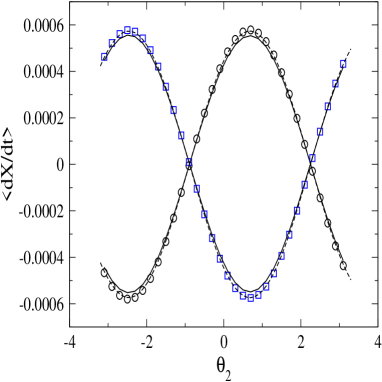
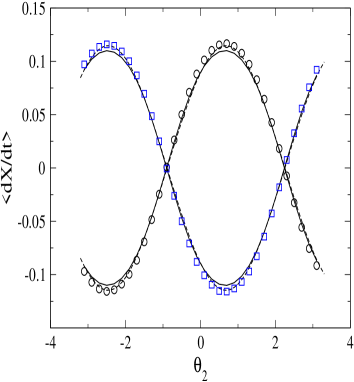
Figure 6: Dependence of the average velocity on $\theta_{2}$ for $m=2$. Left panel: Parameters are $\epsilon_{1}=\epsilon_{2}=0.02$. Right panel: $\epsilon_{1}=\epsilon_{2}=0.2$. Other parameters are $\beta=0.05$, $\delta=0.1$. In both panels two values for $\theta_{1}$ are considered: blue squares are the results of the numerical simulations for $\theta_{1}=0$, and black circles correspond to $\theta_{1}=\pi/2$. Solid lines correspond to the numerical solution of the CC Eqs. (6)-(7). In the left (right) panel dashed lines correspond to $\epsilon\langle\dot{X}_{1}\rangle$ ($\epsilon\langle\dot{X}_{1}\rangle/5$), obtained from Eq. (23).

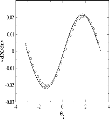
Figure 7: Dependence of the average velocity on $\theta_{2}$ for $m=4$. Circles correspond to numerical simulations; solid line to the numerical solution of CC Eqs. (6)-(7), and dashed line stands for $\epsilon^{2}\langle\dot{X}_{2}\rangle/9$. Parameters are $\epsilon_{1}=\epsilon_{2}=0.2$, $\theta_{1}=0$, $\delta=0.1$ and $\beta=0.05$.

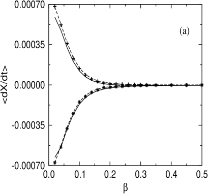
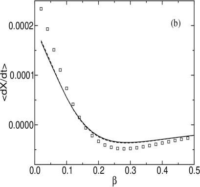
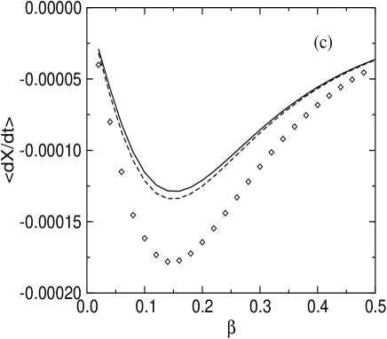
Figure 8: Average velocity of a sG kink as a function of the dissipation for $\beta\geq 0.02$. Panel (a): $\epsilon_{1}=\epsilon_{2}=0.02$, $\delta=0.1$, $\theta_{1}=\pi/2$; Numerical simulations: $\theta_{2}=\pi$ ($\ast$); $\theta_{2}=0$ (+). Panel (b): $\epsilon_{1}=0.04$, $\epsilon_{2}=0.026$, $\delta=0.25$, $\theta_{1}=-\pi/2$, $\theta_{2}=-\pi/2+0.8$; Numerical simulations: ($\square$). Panel (c): $\epsilon_{1}=0.04$, $\epsilon_{2}=0.026$, $\delta=0.25$, $\theta_{1}=-\pi/2$, $\theta_{2}=-\pi/2$; Numerical simulations: ($\lozenge$). In each figure the solid line shows $\langle V\rangle$ obtained from the numerical solution of Eqs. (6)-(7), and the dashed line is $\langle V\rangle$ calculated from Eq. (23).

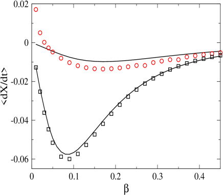
Figure 9: Average velocity of a sG kink as a function of the dissipation for $0.01\leq\beta\leq 0.45$ and for two different frequencies: $\delta=0.1$ (squares); $\delta=0.25$ (circles). The other parameters are $\epsilon_{1}=0.2$, $\epsilon_{2}=0.12$, $\theta_{1}=-\pi/2$, $\theta_{2}=-\pi/2$. In both cases the solid lines show the results obtained from the numerical solution of Eqs. (6)-(7).

III.1 Sine-Gordon model

Our first comparison between the CC analyisis and the numerical simulations is presented in Fig. 1(b), where the time evolution of the center of the kink is presented. As can be seen from the plot, the agreement between our analytical approximation and the numerical results is excellent, even for long times, suggesting that we can be confident that the CC approach captures the ratchet dynamics of the system. Nevertheless, to complete the analysis and fully confirm our analytical predictions, it is crucial to understand how the width of the kink evolves when it is driven by the bi-harmonic external force. The evolution in time of the width of the kink as obtained from the numerical simulations of the full sG equation and from the CC equations are compared in the left panel of Fig. 2. Once again, we observe an excellent agreement between simulations and the CC framework. In order to validate our predictions about the resonance criterion, we proceed to the determination of the Fourier components for the oscillations of the width of the kink (see right panel of Fig. 2). The Discrete Fourier Transform (DFT) shows an excelent agreement between the numerical simulations of Eq. (1) and the numerical solutions of Eqs. (6-7), confirming the resonance criterion. For instance, we can observe that, for $m=2$, the spectrum of $l(t)$ contains the frequencies $\delta$ and $2\delta$, the same frequencies of the bi-harmonic external force. Consequently, one could expect a net motion of the soliton, as was pointed out in Table 2 and as the numerical simulations show. To further confirm the resonance criterion, we analyze the spectrum of $l(t)$ for $m=3,4$, plotted in Fig. 3. For $m=3$ neither $\delta$ nor $3\delta$ appear in the spectrum, thus confirming our predictions (see Table 2): We observe only the presence of even harmonics, and hence we expect an oscillatory motion of the center of the kink similar to that obtained for a force with only one harmonic component niurka5 . Conversely, for $m=4$ we observe the appearance of frequencies $\delta$ and $4\delta$. Therefore, the occurrence of a net motion is also expected as in case of $m=2$ and is indeed confirmed by the simulations (not shown).

Having verified our resonance criterion for the ocurrence of ratchet phenomena, we now turn to discussing how the average velocity depends on the parameters of the ac force and damping. In Fig. 4 we plot the average velocity of the kink, computed from the numerical simulations of the full PDE, for $m=2,3$, and $4$ versus the phase of the second harmonic $\theta_{2}$ [see Eq. (2)]. In this plot, the predictions for the existence or not of motion for different values of $m$ are confirmed. Notice the sinusoidal dependence of the mean velocity on the phase, as predicted by the expressions (23) and (27). Another relevant feature of Fig. 4 is the difference of the mean velocity between the cases $m=2$ and $m=4$. In principle, net motion can occur for any even value of $m$; however, we observe that the maximum of the velocity decreases when $m$ is increased. This can be understood from Eqs. (24) and (28), which predict that $\langle V\rangle\sim\epsilon_{1}^{2}\epsilon_{2}$ for $m=2$ and $\langle V\rangle\sim\epsilon_{1}^{4}\epsilon_{2}$ for $m=4$. For greater values of $m$, $\langle V\rangle\sim\epsilon_{1}^{m}\epsilon_{2}$ ricardo , so if $\epsilon_{1}$ and $\epsilon_{2}$ are small enough, the velocity goes to zero as $m$ is increased. Furthermore, the amplitudes of the peaks of the DFTs corresponding to the frequencies $\delta$ and $2\delta$ for $m=2$ are greater than their counterparts for $m=4$, $\delta$ and $4\delta$ (see right panel of Figs. 2 and 3). In this figure we also notice that there are some values of the phase $\theta_{2}$ for which there is no net motion: For example, for $m=2$, these values are approximately given by $\theta_{2}^{c}=-0.9+n\pi$ ($n=0,1,...$). We will refer to those values of the phase for which there is no net motion as critical values. For $m=2$, the whole set of critical phase values as a function of dissipation and frequencies is provided by the expression $\theta_{2}^{c}=-\Phi_{1}(\beta,\delta)+n\pi$. These correspond to those values of the phase for which the condition (26) is not fulfilled.

The dependence of $\Phi_{1}(\beta,\delta)$ on the dissipation coefficient and the frequency of the ac force is shown in Fig. 5. The figure shows that for the largest value of the frequency, the agreeement between the CC theory and the simulations of the full partial differential equation is only qualitative. The reason for this lies in the fact that, when the harmonics of the ac force contain the frequencies $\delta$ and $2\delta$, the width of the kink is excited with frequencies $2\delta$ and $4\delta$, respectively (because of the term $P^{2}$ in (7), see also previous studies niurka2 ; niurka3 ). If we chose $\delta=0.25$, $l(t)$ will oscillate with $2\delta=0.5$, $4\delta=1$, or even higher frequencies, which are inside the phonon band, which lies above unit frequency. Therefore, for large enough amplitude of the force and small dissipation, strong excitation of phonons is expected (even kink-antinkinks can appear) and correspondingly the failure of our CC approach, since it does not take into account the phonon contribution to the motion. This is yet another reason why simulations for very low values of the dissipation coefficient (and hence with larger phonon production) are not considered in the plot.

Let us now concentrate on the $m=2$ case and compare the average velocities as a function of $\theta_{2}$, computed from the direct numerical simulations of Eq. (1) and from the numerical solution of the CC equations (6)-(7). In Fig. 6 we observe an excellent agreement between these two average velocities. In the left panel, overimposed to these values, we show also the approximate values of $\langle V\rangle$ obtained from Eq. (23). In the right panel, the amplitudes of the two harmonics have been increased by one order of magnitude; this leads to noticeable phonon production in the simulations and consequently to a quantitative disagreement between the simulations and the CC approach, and therefore a factor $1/5$ has been introduced in order to adjust the values of $\langle V\rangle$ obtained from Eq. (23) to the results of the numerical simulations and the numerical solution of CC equations (as is obvious, the qualitative agreement is perfect and in particular for the critical phase values the agreement is quantitative). For the case $m=4$ the situation is the same: There is good agreement between the results of the CC equations and the simulations, although once again the analytical expression $\langle V\rangle$ fits only qualitatively to the numerical results (see Fig. 7).

One important point, relevant in experimental contexts, is the prediction of the CC theory about the dependence of the mean velocity on the dissipation coefficient. According to the standard behavior of point particles under friction, one would expect a monotonic decreasing of the average velocity to zero as a function of the damping. However, the existence of an optimal damping for the occurrence of net motion, and the appeareance of current reversal upon varying the damping (see Salerno-mixing , salerno2 ), show a richer and more complex behaviour in the case of the soliton ratchets we are discussing, depending on the parameters of the ac force. These phenomena, expected also from Eqs. (23) and (27), are shown in Fig. 8, where for the first sets of parameters (Fig. 8a) we observe that the velocity drastically decreases to zero as $\beta$ is increased. Notice that in this case the time-reversal symmetry of the ac force is broken in the optimal way ricardo by the given phases. In Fig. 8c, when the phases are chosen in a manner such that the time reversal symmetry $f(t)=f(-t)$ is fulfilled in the absence of dissipation, an optimal value of $\beta$ for the transport is observed. In this case, when the dissipation coefficient increases starting from $\beta=0$, the time-reversal symmetry begins to break, and therefore an increase of the average velocity is expected. On the other hand, increasing the damping tends to suppress any motion. Hence, in between these two opposite mechanisms an optimal value of the damping must appear ricardo . Between these two limit cases, we can see the appeareance of current reversal (see Fig. 8b) as was pointed out in Salerno-mixing .

From Fig. 8 we can see that the best agreement between CC theory and numerical simulations is obtained for small values of the frequencies of the ac force. Indeed, in Fig. 8c, for $\delta=0.25$, due to the phonon contribution (see the discussion above), we observe only a qualitative agreement between the numerical simulations and the CC theory. This disagremeent is even clearer in Fig. 9, where we take large values of the amplitudes of the ac force and compare the mobility of the kink for $\delta=0.1$ and $\delta=0.25$. We can observe that for the largest value of frequency together with the smallest values of $\beta$ the results from the theory do not fit quantitatively the values obtained from the numerical simulations. Furthermore, we even observe current reversal in the results of the numerical simulations, contrary to the predictions of the CC theory. As we explained above, this disagreement arises from the large production of phonons for this value of the frequency, unaccounted for in the CC approach.

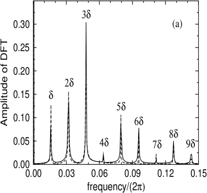
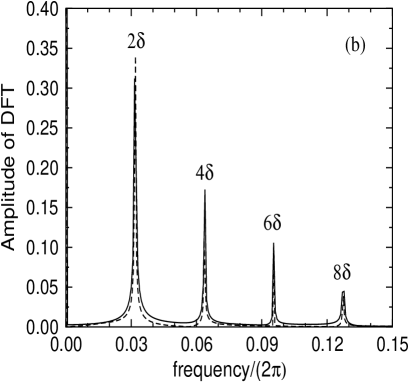
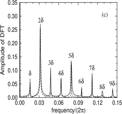
Figure 10: Discrete Fourier Transform of the width of a $\phi^{4}$ kink. (a): $m=2$; (b): $m=3$; (c): $m=4$. Solid line: Simulations of Eq. (3). Dashed line: numerical integration of the CC equations.

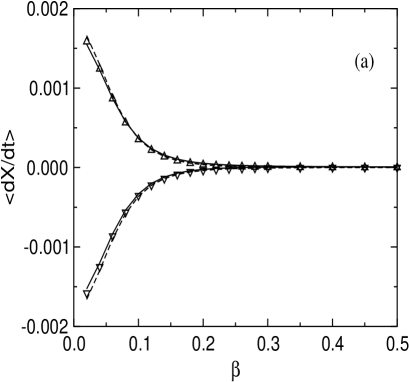
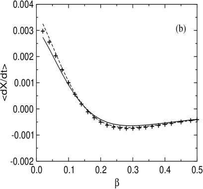
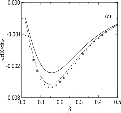
Figure 11: Average velocity of a $\phi^{4}$ kink as a function of the dissipation for $\beta\geq 0.02$. (a): $\epsilon_{1}=\epsilon_{2}=0.02$, $\delta=0.1$, $\theta_{1}=\pi/2$. Numerical simulations: $\theta_{2}=\pi$ ($\triangledown$); $\theta_{2}=0$ ($\vartriangle$). (b): $\epsilon_{1}=0.04$, $\epsilon_{2}=0.026$, $\delta=0.25$, $\theta_{1}=-\pi/2$, $\theta_{2}=-\pi/2+0.8$. Numerical simulations: (+). (c): $\epsilon_{1}=0.04$, $\epsilon_{2}=0.026$, $\delta=0.25$, $\theta_{1}=-\pi/2$, $\theta_{2}=-\pi/2$; Numerical simulations: ($\times$). In all cases the solid lines show results obtained from the numerical solution of Eqs. (6)-(7) and the dashed lines are the values obtained from Eq. (23).

III.2 $\phi^{4}$ model

After describing in the previous subsection the ratchet dynamics of kinks in the sG equation, here we focus our attention on the $\phi^{4}$ model. This is important in order to ascertain to what extent does the phenomenology found depend on the unperturbed equation being integrable, or on the structure of the sG soliton (which, for instance, does not have internal modes modosinternos , whereas the $\phi^{4}$ model does have one). In view of this, we carried out numerical simulations of the $\phi^{4}$ model, to compare with the analytical CC results in Sec. II. As we will now summarize, the phenomenology of directed motion of kinks in the $\phi^{4}$ model is the same as in the sG model.

To begin with, we can observe in Fig. 10 that our first resonance criterion on the synchronization between the oscillations of $l(t)$ and $f(t)$ does also apply for the $\phi^{4}$ model. As we can see, for even value of $m$ ($m=2,4$) there are resonant frequencies, while in case of $m=3$ the frequencies of the ac force $\delta$ and $3\,\delta$ never appear in the spectrum of the width of the kink. Correspondingly, in our numerical simulations we have found unidirectional motion only in cases of $m=2,m=4$, in contrast to $m=3$ where an oscillatory motion of the center of the kink takes place (not shown). The sinusoidal dependence of the average velocity on the phases is found as well as in the sG equation. The other feature we focused on, namely dissipation effects, agrees with the previous picture as well: In Fig. 11 we observe, as in the sG case, that changing the damping we can decrease the average of the velocity, rectify the motion, or optimize it. In this respect, another interesting issue is the comparison between the observed mobility of the kink between the sG and $\phi^{4}$ models. From Eq. (29), it can be noticed that, if we consider the first approximation of $l(t)$, the center of the kink will feel an ac force with the amplitudes of the two harmonics modulated by the factor $\lambda=q/M_{0}$, which in sG is $\lambda_{sG}=0.785$ and in $\phi^{4}$, $\lambda_{\phi 4}=2.121$. Therefore, for the same values of $\epsilon_{i}$ in both systems, the effective amplitude of the ac force that the center of the kink experiences in $\phi^{4}$ is greater than in sG, $\lambda_{sG}\epsilon^{sG}_{i}<\lambda_{\phi 4}\epsilon^{\phi 4}_{i}$. Therefore, from the CC analysis we expect higher mobility for the $\phi^{4}$ model, which is in good agreement with the numerical simulations as is shown in Figs.  8 and 11. We thus conclude that the existence of net motion of kinks (topological excitations) is a generic phenomenon, both in terms of the criterion for its appearance and its main characteristics, and not a specific feature of the sG equation.

IV Conclusions

In this paper we have investigated in detail the behavior of topological excitations when driven by ac forces in homogeneous systems. We have focused on the nonlinear Klein-Gordon family of models as a paradigmatic example, and specifically on the sG and $\phi^{4}$ equations as examples of integrable and non-integrable models, respectively. By means of an analytical technique of the CC class, we have shown that two conditions must be fulfilled in order to observe unidirectional motion of the kinks: First, the shift symmetry must be broken, and second the time-reversal symmetry must be broken as well. In the absence of dissipation, the first symmetry may be violated by a bi-harmonic force containing even and odd harmonics of the frequency. We have devoted a large part of our work to characterize the case in which the force is composed of the first and second harmonics [$m=2$ in Eq. (2)], and we have found that the velocity of the net motion depends on the relative phase between the two harmonic forces in a sinusoidal manner. The values of the phase for which the velocity vanishes (critical phase values) are precisely those for which, loosely speaking, the breaking of the time-reversal symmetry by the ac force is compensated by the breaking of the time-reversal symmetry due to the damping. Numerical simulations for the two models considered are in very good agreement with the analytical results, qualitatively in terms of the velocity value, and quantitatively as far as the critical phase values are concerned. We have also studied the cases of the third ($m=3$) and fourth ($m=4$) harmonics, finding, respectively, no motion (because the shift symmetry is not broken) and motion slower than in the previous case. Indeed, as we have seen, in general the efficiency of the driving diminishes when the second harmonic force is a higher harmonic. In all cases, the arguments in terms of shift symmetry breaking forces can be equivalently presented as existence or not of resonant behavior between the frequencies present in the driving and those in the time evolution of the width of the kink.

In addition to the breaking of the time-reversal symmetry of the ac force, we have also studied another form of time-reversal symmetry violation, namely by introducing dissipation in the models. In the presence of dissipation, we have observed three different types of behavior depending on the parameters of the driving: A monotonically decreasing velocity of the kink with increasing dissipation, the appearance of an optimum value of the dissipation with a maximum in the velocity, and even reversals of the directed motion for some values of the dissipation. In all three cases, the CC theory describes correctly the phenomena as observed in the simulation, except when the dissipation is very small, allowing for a non-negligible excitation of phonons in the system that breaks down the basic assumption of the CC theory.

The conclusions we have just summarized acquire greater relevance when compared to different types of experimental results schia ; JJ2 ; optical2 . In the absence of dissipation schia , experiments in optical lattices with biharmonic driving find a sinusoidal dependence on the relative phase similar to the one reported here. When dissipation is present in Josephson junctions JJ2 , the same sinusoidal dependence is again found, and optimal driving parameters appear. Finally, recent work on dissipation effects on optical lattices optical2 exhibits several of the features we have just discussed, such as the dependence of the critical phase on the damping, and the overall sinusoidal dependence. Although the motion of cold atoms is essentially based on a one-particle description the dissipation in the system is caused by ground state transitions, which manifests the presence of an internal dynamics. The role of this internal dynamics for the ratchet mechanism in cold atoms has been put forward in Mennerat . In this regard the role of the internal mode in our CC approach could shed light on the effect of the interband transitions and their disipative effects in the ratchet transport of cold atoms. We thus see that our results are very generic, in so far as they apply to a large family of theoretical models, both integrable and non-integrable, and they capture the essential ingredients of experiments in different fields ricardo . Therefore, the main conclusion of our work is that we have correctly identified the mechanism for the appearance of directed motion due to zero-mean forces through the breaking of symmetries, and we have provided a physical interpretation of this mechanism in terms of the coupling between excitation modes of the system. We hope that this work encourages further experimental work to check the remaining features discussed.

- (1) P. Hänggi and R. Bartussek, in Nonlinear Physics of Complex Systems — Current Status and Future Trends, edited by J. Parisi, S. C. Müller, and W. Zimmermann (Lecture Notes in Physics no. 476, Springer, Berlin, 1996).
- (2) R.D. Astumian and P. Hänggi, Physics Today 55 (11), 32 (2002).
- (3) F. Jülicher, A. Ajdari, and J. Prost, Rev. Mod. Phys. 69, 1269 (1997).
- (4) P. Reimann, Phys. Rep. 361, 57 (2002).
- (5) H. Linke, editor, Ratchets and Brownian Motors: Basics, Experiments and Applications, Appl. Phys. A 75 (special issue).
- (6) P. Hänggi, F. Marchesoni, and F. Nori, Ann. Phys. (Leipzig) 14, 51 (2005).
- (7) C. R. Doering, Nuovo Cimento Soc. Ital. Fis., D 17, 685 (1995).
- (8) A. Ajdari, D. Mukamel, L. Peliti, and J. Prost, J. Phys. I France 4, 1551 (1994).
- (9) S. Flach, O. Yevtushenko, and Y. Zolotaryuk, Phys. Rev. Lett. 84, 2358 (2000).
- (10) S. Savel’ev, F. Marchesoni, P. Hänggi, and F. Nori, Europhys. Lett. 67, 179 (2004); Phys. Rev. E 70, 066109 (2004).
- (11) M. Borromeo, P. Hänggi and F. Marchesoni, J. Phys. Condens. Matter 17, S3709 (2005).
- (12) F. Marchesoni, Phys. Rev. Lett. 77, 2364 (1996).
- (13) S. I. Denisov, E. S. Denisova, and P. Hanggi, Phys. Rev. E 71, 016104 (2005).
- (14) L. Morales-Molina, F.G. Mertens and A. Sánchez, Eur. Phys. J. B 37, 79 (2004); Phys. Rev. E 72, 016612 (2005).
- (15) M. Schiavoni, L. Sánchez-Palencia, F. Renzoni, and G. Grynberg., Phys. Rev. Lett. 90, 094101 (2003).
- (16) I. Zapata, J. Luczka, F. Sols and P. Hänggi, Phys. Rev. Lett. 77, 2292 (1996).
- (17) E. Goldobin, A. Sterck, and D. Koelle Phys. Rev. E 63, 031111 (2001).
- (18) A. V. Ustinov, C. Coqui, A. Kemp, Y. Zolotaryuk, and M. Salerno, Phys. Rev. Lett. 93, 087001 (2004).
- (19) P. Reimann, M. Grifoni, and P. Hänggi, Phys. Rev. Lett. 79, 10 (1997); M. Grifoni, M. S. Ferreira, J. Peguiron, and J. B. Majer, Phys. Rev. Lett. 89, 146801 (2002); J. B. Majer, J. Peguiron, M. Grifoni, M. Tusveld, and J. E. Mooij, Phys. Rev. Lett. 90, 056802 (2003); A. Sterck, R. Kleiner, and D. Koelle, Phys. Rev. Lett. 95, 177006 (2005).
- (20) R. Gommers, S. Bergamini, and F. Renzoni, Phys. Rev. Lett. 95, 073003 (2005).
- (21) R. Chacón and N. R. Quintero, arXiv:physics/0503125 (2005).
- (22) S. Flach, Y. Zolotaryuk, A.E. Miroshnichenko, and M.V. Fistul, Phys. Rev. Lett. 88, 184101 (2002).
- (23) M. Salerno and Y. Zolotaryuk, Phys. Rev. E 65, 056603 (2002).
- (24) I. Goychuk and P. Hänggi, J. Phys. Chem. B 105, 6642 (2001).
- (25) A. C. Scott, Nonlinear Science (Oxford University, Oxford, 1999).
- (26) N.R. Quintero, A. Sánchez, Phys. Lett. A 247, 161 (1998); Eur. Phys. J. B 6, 133 (1998).
- (27) E. Goldobin, B. A. Malomed, and A. V. Ustinov, Phys. Rev. E 65, 056613 (2002).
- (28) L. Morales-Molina, N.R. Quintero, F.G. Mertens, and A. Sánchez, Phys. Rev. Lett. 91, 234102 (2003).
- (29) A. Sánchez and A. R. Bishop, SIAM Rev. 40, 579 (1998).
- (30) M.J. Rice and E.J. Mele, Solid State Commun. 35, 487 (1980); M.J. Rice, Phys. Rev. B 28, 3587 (1983).
- (31) N.R. Quintero, A. Sánchez, and F.G. Mertens, Phys. Rev. E 62, 5695 (2000).
- (32) N.R. Quintero, A. Sánchez, and F.G. Mertens, Phys. Rev. Lett. 84, 871 (2000).
- (33) N.R. Quintero, B. Sánchez-Rey, and J. Casado-Pascual, Phys. Rev. E 71, 058601 (2005).
- (34) S. Denisov, et al. Phys. Rev. E 66, 041104 (2002).
- (35) M. Salerno and N.R. Quintero, Phys. Rev. E. 65, 025602, (2002); N.R. Quintero, B. Sánchez-Rey, and M. Salerno, Phys. Rev. E 72, 016610 (2005).
- (36) S. Denisov, S. Flach, and A. Gorbach, Europhys. Lett. 72, 183 (2005).
- (37) W. A. Strauss and L. Vázquez, J. Comput. Phys. 35, 61 (1990).
- (38) N. R. Quintero, A. Sánchez, and F. G. Mertens. Eur. Phys. J. B 19, 107 (2001).
- (39) N.R. Quintero, A. Sánchez, and F.G. Mertens, Phys. Rev. E 62, R60 (2000).
- (40) C. Mennerat-Robilliard, D. Lucas, S. Guibal, J. Tabosa, C. Jurczak, J.-Y. Courtois, and G. Grynberg, Phys. Rev. Lett. 82, 851 (1999).