Asymptotic analysis of the model for distribution of high-tax payers

Abstract

The z-transform technique is used to investigate the model for distribution of high-tax payers, which is proposed by two of the authors (K. Y and S. M) and othersKyamamoto ; Kyamamoto2 ; Kyamamoto3 . Our analysis shows an asymptotic power-law of this model with the exponent -5/2 when a total “mass” has a certain critical value. Below the critical value, the system exhibits an ordinary critical behavior, and scaling relations hold. Above the threshold, numerical simulations show that a power-law distribution coexists with a huge “monopolized” member. It is argued that these behaviors are observed universally in conserved aggregation processes, by analizing an extended model.

Key words: power-law distribution, high income model, asymptotic analysis

1. Introduction

Some years ago, two of the authors (K. Y and S. M) et al Kyamamoto ; Kyamamoto2 ; Kyamamoto3 proposed a simple model for distribution of high-tax payers. They considered a 2-body interaction system where the winner takes all competing money when the competition occurs. Their model is regarded as a simple aggregation system, which is widely discovered in various systems in nature and, naturally, has been attracted considerable interest by many researchersley ; Schmelzer . Their simulation gives the universal power-law distribution, and shows a good fit with the date in Japan and the United States’ CEO’s. However they could not succeed in theoretical derivation of obtained results.

We analyze their model mathematically, and derive an asymptotic expression of the probability distribution functions. In the model, the total number of units (mass) is conserved, and plays a role of a control parameter. The distribution function obeys the power-law at a certain critical value. Below the critical value, the system exhibits an ordinary critical behavior, and scaling relations hold. Above the threshold, numerical simulations show that a power-law distribution coexists with a huge “monopolized” member. These bahaviors are agreed with the phase transision of the non-conserved process discussed by Krapivsky and RenderRedner and Majumdar et alMajum .

2. Model and Analysis

The model introduced by Yamamoto et al, is defined by the following competition processes and conservation conditions:

C1. The system consists of N homogeneous members. The number N is fixed.

C2. The system holds $S$ units as resource money. Each member holds one unit as a minimum amount. The total amount $S$ is conserved.

P1. Two members, who are picked at random from the whole membership transact an economic activity competitively. The winner collects the whole of the competing money and the loser loses all one’s money. In order to keep the number of active members constant, one unit is added to the loser.

P2. To preserve the total resource money, one unit is reduced from a member who is picked at random and has resource money more than or equal to 2 units.

We analyze this model by using the z-transform technique and calculate the probability distribution function $P(X)$ that an arbitrarily chosen member holds X units of resource money. At steady-states, the equations for $P(X)$ read

$$(1-P(1))(1-P(1))+\frac{P(2)}{1-P(1)}= (P(1))^{2}\;\;(X=1),$$ (1)

$$\sum_{i+j=X}P(i)P(j)+\frac{P(X+1)}{1-P(1)}=2P(X) +\frac{P(X)}{1-P(1)}\;\;(X\geq 2).$$ (2)

Note that $\sum_{X}P(X)=1$ for normalization. For the analysis of the equation of this kind, it is useful to consider the z-transform $\phi(z)$ of $P(X)$:

$$\phi(z)=\sum_{X=0}^{\infty}P(X)z^{-X}.$$ (3)

Here it is defined that $P(0)=0$. From the normalization condition, $\phi(z)$ must satisfy $\phi(1)=1$. Taking the z-transform of Eq.(2) and Eq.(1), we get the basic equations in z-space as,

$$\{1-P(1)\}\phi^{2}(z)+\{z-3+2P(1)\}\phi(z)-P(1)+\frac{1}{z}=0.$$ (4)

We can now analyze $P(1)$ by differentiation Eq.(4) with respect to $z$. Differentiating once and substituting $z=1$, we simply get the identity. Next differentiation leads to the equation about $\phi^{\prime}=\phi^{\prime}(1)$,

$$\{1-P(1)\}\phi^{\prime 2}+\phi^{\prime}+1=0.$$ (5)

Note that $-\phi^{\prime}(1)=\sum XP(X)=S/N$ is the average of resource units, and is conserved in processes. We employ $-\phi^{\prime}$ as the control parameter of the system. Once $-\phi^{\prime}$ is given, $P(1)$ can be determined via Eq.(5). Fig.  1 shows $P(1)$ versus $-\phi^{\prime}$. It becomes evident that $1\geq P(1)\geq\frac{3}{4}$, and generally $P(1)$ corresponds to two values $\phi_{A}$ and $\phi_{B}$ of $-\phi^{\prime}$, in the region A: $1\leq\phi_{A}\leq 2$ and B: $2<\phi_{B}$.

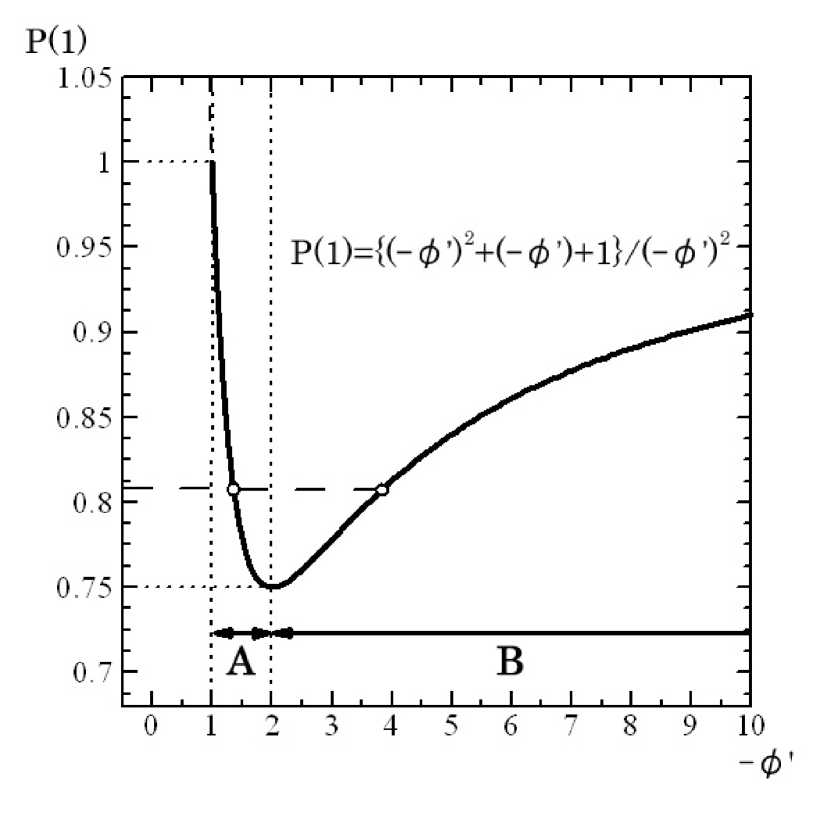
Figure 1: Value of $P(1)$ versus the control parameter $-\phi^{\prime}$. $P(1)=1$ means that all the member have one unit.

Note that from the definition of the system, each member should have at least one unit thus $-\phi^{\prime}=1$ is the minimum value.

First, we treat the case where $-\phi^{\prime}=2$ and Eq.(5) has a repeated root, i.e., $P(1)=3/4$. Substituting $P(1)=3/4$ to (4), we have the solution of the quadratic equation

$$\phi(z)=3-2z\pm 2z(1-\frac{1}{z})^{\frac{3}{2}}.$$ (6)

The singularity of $\phi(z)$ near $z\sim 1$ is,

$$\phi(z)|_{z\sim 1}\sim 1\pm 2(1-\frac{1}{z})^{\frac{3}{2}},$$ (7)

Then the asymptotic behavior of $P(X)$ at large $X$ is given by

$$P(X)\sim\frac{1}{X^{\sigma}},\;\;\;\sigma=\frac{5}{2}.$$ (8)

This power-law exponent coincides with numerical results of  Kyamamoto .

Next we discuss the behavior of the system with the control parameter $-\phi^{\prime}\neq 2$. The original equations (1), (2) can be solved sequentially if once $P(1)$ is given. In Fig. 2, numerical solutions of Eq.(1) and (2) are plotted for several values of $P(1)$.

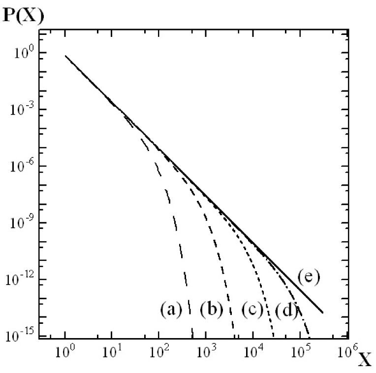
Figure 2: Solutions of $P(X)$ with different values of $P(1)$. (a) $P(1)=0.76$, (b) $P(1)=0.751$, (c) $P(1)=0.7501$, (d) $P(1)=0.75001$, (e) $P(1)=0.75$.

With the values $\phi_{A}$ of $-\phi^{\prime}$ in the region A of Fig. 1, our simulation results agree with these sequential solutions. We conclude that in this region the system has stable steady states, and the solutions of basic equations (1) and (2) represent these stable states.

The behavior of these solutions, which is shown in Fig. 2, is very similar to the ones of ordinary critical phenomena. For arguing this behavior, let $P(1)=\frac{3}{4}+\epsilon$, then analyze the reverse z-transform,

$$\begin{split}P(X)&=\frac{1}{2\pi i}\oint z^{X-1}\phi(z)dz\\ &=\frac{1}{2\pi i}\oint z^{X-1}(z-1)\sqrt{1-\frac{1-4\epsilon}{z}},\end{split}$$ (9)

in the limit $\epsilon\rightarrow 0$. The most singular part of (9) is given by,

$$\begin{split}P(X)&\sim\frac{1}{2\pi i}\oint e^{X\{(z-1)-\frac{(z-1)^{2}}{2}+\cdots\}}(z-1)\sqrt{z-1+4\epsilon}dz\\ &\sim\frac{1}{2\pi i}\oint e^{X\epsilon\alpha}\epsilon\alpha\sqrt{\epsilon\alpha+4\epsilon}\cdot\epsilon d\alpha\\ &\sim X^{-\frac{5}{2}}\Psi(\epsilon X),\end{split}$$ (10)

where the scaling function $\Psi(Y)$ is expressed as,

$$\Psi(Y)=\frac{(Y)^{\frac{5}{2}}}{2\pi i}\oint e^{\alpha Y}\alpha\sqrt{\alpha+4}d\alpha.$$ (11)

We find that ordinary scaling relations hold.

The behavior of $P(X)$ is completely different when the control parameter $-\phi^{\prime}$ is larger than $2$. Fig. 3 shows the simulation result for $N=100000$ and $-\phi^{\prime}=202$. The part of units, about $2\times N$ units, obey the power-law with the exponent $-5/2$, and the rest of them coagulates eventually to one “monopolized” member, represented by the arrow in Fig. 3. Thus this member has almost $m_{R}=(-\phi^{\prime}-2)\times N$ units.

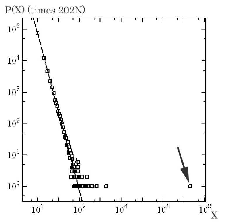
Figure 3: Simulation result for $N=100000$ and $-\phi^{\prime}=202$.

We have also done simulations with different values of $-\phi^{\prime}$ in the range from $3$ to $1002$. In all these simulations $P(X)$ behaves like Figs. 3.

The behavior described above is substantially the same as that of the model reported by Majumdar et alMajum , though thier model is different from the present model for it does not preserve the total mass strictly.

3. Extended Model

Now we argue that systems which exhibit those behaviors are not limited to this particular process. To the end ,we examine the model extended as follows. (i) In the competition process P1, $n$ units are added to the loser. (ii) In the procedure P2, $m$ member with $X\geq 2$ are picked at random and one unit is reduced from each of these member. The case $n=m=1$ corresponds to the original model.

Similarly to the original model, the equations for $P(X)$ at steady state read

$$\frac{mP(2)}{1-P(1)}=2P(1)\qquad(X=1),$$ (12)

$$\sum_{i+j=n}P(i)P(j)+(1-P(n))(1-P(n))+\frac{mP(n+1)}{1-P(1)}=(P(n))^{2}+\frac{mP(n)}{1-P(1)}\qquad(X=n),$$ (13)

$$\sum_{i+j=X}P(i)P(j)+\frac{mP(X+1)}{1-P(1)}=2P(X)+\frac{mP(X)}{1-P(1)}\qquad(X\neq n,X\geq 2).$$ (14)

In z-space, these equations are rewritten as

$$A\phi^{2}(z)+\{m(z-1)-2A\}\phi(z)+m(1-A)\left(\frac{1}{z}-1\right)+\frac{A}{z^{n}}=0,$$ (16)

and the solution of (16) is

$$\phi(z)=\frac{1}{2A}\left(-\{m(z-1)-2A\}\pm\sqrt{D(z)}\right),$$ (17)

$$D(z)=\{m(z-1)-2A\}^{2}-4A\left\{m(1-A)\left(\frac{1}{z}-1\right)+\frac{A}{z^{n}}\right\}.$$ (18)

First we treat the case $n\neq m$. In this case the total amount $S$ of units varies, thus the situation is quite different from the original model. However, the analysis described above is still applicable.

When $n\neq m$, the discriminant $D(z)$ is

$$D(z)=(z-1)f(z),\qquad f(1)\neq 0.$$ (19)

The singularity of $\phi(z)$ near $z\sim 1$ is $\phi(z)|_{z\sim 1}\sim 1\pm\{(n-m)(z-1)\}^{1/2}$. It gives a familiar power-law distribution (for example, see ley ; takayasu ),

$$P(X)\sim\frac{1}{X^{\sigma}},\;\;\;\sigma=\frac{3}{2}.$$ (20)

When $n<m$, the total amount $S$ eventually vanishes. However if we take $S$ large enough, our simulation shows the temporal power-law distribution with the exponent $-3/2$. Also in the case $n>m$, the range of the power-law distribution with the exponent $-3/2$ continually extends like $\sqrt{t}$ as the time $t$ goes on.

In the case $n=m$, $-\phi^{\prime}(1)=-\phi^{\prime}$ can be used as the control parameter, as the original model, since $S$ is conserved. When $-\phi^{\prime}=2$,

$$P(1)=1-A=\frac{1}{2(n-1)}\left\{2n-\sqrt{2n^{2}-2n+4}\right\},$$ (21)

and

$$D(z)=(z-1)^{3}g(z),\qquad g(1)\neq 0.$$ (22)

Thus, the asymptotic behavior of $P(X)$ at large $X$ is given by

$$P(X)\sim\frac{1}{X^{\sigma}},\;\;\;\sigma=\frac{5}{2}.$$ (23)

It is just the same exponent as the original model. Also our simulations show that the behavior when $-\phi^{\prime}\neq 2$ is essentially the same as the original.

4. Discussion

These models show drastic change of behavior as the control parameter $-\phi^{\prime}$ varies. When $-\phi^{\prime}>2$, once the “monopolized” member appears our simulation shows this member does not exchange with other members after that. It is practically stable, so we believe that this transition is not only the normal static phase-transition, but also the dynamic “ergodic-nonergodic” transition.

Our analysis described above shows that the exponent of “power-law” part does not change in two models. Furthermore, it can be shown analytically that the exponent of the power-law depends only on conservation conditions when the kernel is constant. These studies suggest strongly that the behavior described above is observed universally in conserved aggregation processes. We believe this analysis gives clues for classification of these conserved aggregation processes.

We thank Prof. S. Redner for pointing out references Redner and Majum to us.

References

- (1) P. L. Krapivsky and S. Render, Phys. Rev. E 54, 3553 (1996).
- (2) F. Leyvraz, Phys. Rep. 383, 95 (2003).
- (3) Satya N. Majumdar, Supriya Krishnamurthy, and Mustansir Barma, Phys. Rev. Lett. 81, 3691 (1998).
- (4) J. Schmelzer, G. Röpke and R. Mahnke, Aggregation Phenomena in Complex Systems. Wiley-Vch (1999).
- (5) H. Takayasu, I. Nishikawa and H. Tasaki, Phys. Rev. A 37, 3110 (1988).
- (6) K. Yamamoto, S. Miyazima, R. K. Koshal, M. Koshal and Y. Yamada, Japan J. Indust. Appl. Math. 20, 147-154 (2003).
- (7) K. Yamamoto, S. Miyazima, R. K. Koshal, Y. Yamada, Physica A 314, 743-748 (2002).
- (8) K. Yamamoto, S. Miyazima, H. Yamamoto, T. Ohtsuki and A. Fujihara, Practical Fruits of Econophysics, Springer, 349 (2006).