Conductance Phases in Aharonov-Bohm Ring Quantum Dots

Abstract

The regimes of growing phases (for electron numbers $N\approx 0-8$) that pass into regions of self-returning phases (for $N>8$), found recently in quantum dot conductances by the Weizmann group are accounted for by an elementary Green function formalism, appropriate to an equi-spaced ladder structure (with at least three rungs) of electronic levels in the quantum dot. The key features of the theory are physically a dissipation rate that increases linearly with the level number (and tentatively linked to coupling to longitudinal optical phonons) and a set of Fano-like meta-stable levels, which disturb the unitarity, and mathematically the change over of the position of the complex transmission amplitude-zeros from the upper-half in the complex gap-voltage plane to the lower half of that plane. The two regimes are identified with (respectively) the Blaschke-term and the Kramers-Kronig integral term in the theory of complex variables.

PACS numbers: 03.65.Vf

Keywords: Quantum dots, Aharonov-Bohm effect, Green function, Hilbert Transform.

1 Two Phase Regimes

Following a theoretical prediction in [2], a pioneering experimental determination of the phase evolution in quantum dots subject to the Aharonov-Bohm effect was made by the Heiblum-led Weizmann group, as e.g. in [3]-[7]. The same group has recently come up with an interesting development and a physical description [8], which throw fresh light on their results (previous and recent). They showed (cf. their figures 4-6) that as the gate voltage ($V_{p}$ in their notation) increases and more electrons are entering the quantum dot, the phase of the conductance evolves in the following manner:

Initially, for a number of electrons N in the quantum dot up to 8 ($N\leq 8$) the phases corresponding to each N increase in a stepwise fashion, following which, as $N>8$, the phases return continuously to their original value (make a phase lapse).

Other manifestations of the absence of ”phase rigidity” (meaning, the discontinuous switch of phases between $0$ and $\pm\pi$ , connected to unitarity) in the phase-coherent transport across quantum dots were observed in [9].

On the theoretical front, the unexpected phase-behavior of the experiments have resulted in numerous theoretical efforts, several of which included investigation of the Kondo-effect (e.g., [10]). Other works were directed at an analysis of the results in terms of the Landauer-Büttiker formalism of conductivity, which then led to consideration of the transmission amplitude $t^{QD}(U)$ as function of the gap voltage U [11]-[15]. The complicated geometry of the experiments necessitated the inclusion in the theory of several channels and the couplings between these [16], as well as a detailed analysis of the phase that was being observed [17]. A qualitative effect of changes in both the transmission probability and the phase was theoretically found when the signs were changed in some dot-lead coupling matrix elements[18]. More recently, the ingoing-outcoming coupling asymmetry was studied more comprehensively, again in a two level system [19]. A selective choice of the experimental phase-conductance results obtained in [6, 7] was matched with use of the Friedel sum rule in [20], without accounting for the transition between the phase-growth and the phase lapse regimes.

Quantum dot-ring transmission is theoretically related to transmission in quantum wave-guides [12, 13]. The latter was studied in [21]-[23], which noted the existence of pole-zero pairs in the transmission amplitude (as function of the incident wave energy), and especially the changes that occurred with resonant attachments (stubs) to the wave guide. An interesting finding was made in [22], that in wave-guides some geometric changes (like attaching stubs) are formally equivalent to coupling between discrete and a continuum of states (the Fano-effect [24]). For Aharonov-Bohm interferometric devices including quantum dots the interrelation between geometry and Fano-states was formulated in [25], and recent experiments were interpreted in terms of the Fano-effect [9]. We stress here this theoretical equivalence, since many previous explanations of the anomalous phase-behavior in quantum dots concentrated on the geometrical aspect, whereas in the following theory the breakdown of unitarity is traced to decay of conducting levels and to the meta-stability electronic states lying above the quantum dot well. The essential modification that this paper makes in the previous treatments of the Fano-effect is thus that the higher-lying states are assumed to possess a short life time, so that the imaginary part dominates the energy denominator. (Under this assumption it makes no difference whether the higher lying states form a continuum or are discrete, as we propose for simplicity.) Establishing the causes of the meta-stability of the high lying states and of the level-dependent decay rate in the lower lying states is not a primary aim of this work, which is largely phenomenological. Certain considerations indicate that both are due to coupling to longitudinal optical (LO) phonons and this speculative idea is described in section 5.

Though apparently far removed from the physics of quantum dots, it turns out the the question of zeros and poles of the transmission amplitude or of a Greens function (the equivalence between which was demonstrated in [23]) plays an important role in the explanation of the phase behavior. This was heralded in several previous works (e.g., [26]), but the present theory does this in a more comprehensive form, namely by use of Hilbert transform (in section 3) and through a compact representation of the transmission amplitude (in section 4) .

Though the simple theory presented below is implemented by ad hoc assignment of some parameter values and needs to be amplified to fill in several physical details, it seems that it contains the answer to the question: What lies behind the strange phase behavior? A view expressed in [8] is that the so far available theories are short of providing an answer [27]. Earlier experimental data of [5] for returning phases were rather precisely correlated with the observed conductivities by the present authors, using a parameter-free method which was the precursor of the present work [28]. In the Conclusion section of this work, we summarize the differences between the here proposed theory and those of other researchers.

2 Electron Transmission Amplitude

The properties of the quantum dot (spin-less) electron transmission function can be best understood in terms of the theory of Hackenbroich and Weidenmuller [11]. For the sake of completeness we repeat here their end result.

2.1 System Hamiltonian

The system under consideration is composed of three sub-systems:

1. The leads.

2. The Aharanov-Bohm system not containing the dot.

3. The quantum dot.

The entire Hamiltonian of the system can be described by:

$$H=H_{0}+H_{T}$$ (1)

$H_{0}$ describes the totally disconnected system and is given by:

$$H_{0}=\sum_{akr}\epsilon_{ak}^{r}c_{ak}^{r{\dagger}}c_{ak}^{r}+\sum_{i}\epsilon_{i}d_{i}^{{\dagger}}d_{i}+\sum_{j}E_{j}q_{j}^{{\dagger}}q_{j}+U_{ES}$$ (2)

$r$ denotes the leads, $a$ runs over the channels in each lead, $k$ over the longitudinal wave numbers, and $\epsilon_{ak}^{r}$ is the corresponding energy. The energies of the single particle states within the rings and within the dot are labelled by $\epsilon_{i}$ and $E_{j}$ respectively. $E_{j}$ is assumed to depend parametrically on $U$. In the formal theory to follow, $U$ is a complex quantity, whose real part $ReU$ is identified with the experimentally manipulated plunger voltage $V_{p}$. $U_{ES}$ is the electrostatic charging energy of the dot.

The coupling Hamiltonian $H_{T}$ has the form:

$$H_{T}=\sum_{akir}W_{ai}^{r}(k)c_{ak}^{r{\dagger}}d_{i}+\sum_{ijp}V_{ij}^{p}q_{i}^{{\dagger}}d_{j}+H.C.$$ (3)

$W$ describes the coupling between ring and leads, $V$ describe the much smaller coupling between ring and dot. $p=L,R$ labels either side of the dot. In actuality, we should allow for more exit channels than just the two ($L$ and $R$) for the dot, corresponding to the experimental arrangements in, e.g., [8]. We shall account for these by including them in the postulated ”high lying” energy levels (see below in equation (11) and recall the discussion on the equivalence between stub and Fano-states effects in our opening section).

The transmission amplitude $t_{ab}(E)$ through the ring for an electron entering the ring via channel $b$ in lead two, and leaving it via channel $a$ in lead one is derived in [11]. We separate this as

$$t_{ab}=t^{0}_{ab}+t^{QD}_{ab}$$ (4)

into the ring transmission and the transmission $t^{QD}_{ab}$ across the quantum dot and treat first the former.

2.2 Aharonov-Bohm ring transmission

The transmission matrix across the ring is expressed by

$$t^{0}_{ab}=-2i\pi\sum_{ik}W^{1}_{ai}(D^{0})^{-1}_{ik}W^{2*}_{bk}$$ (5)

with the matrix $(D^{0})_{ik}$ defined by:

$$(D^{0})_{ik}=(E-\epsilon_{i})\delta_{ik}+i\pi\sum_{ct}W_{ci}^{t*}W_{ck}^{t}$$ (6)

When the ring is feeded by the lead’s reservoir filled up to the Fermi energy $E_{f}$, one can replace $E$ in equation (6) by $E_{f}$. In the presence of a magnetic field threading the circuit, the ring transmission amplitude will acquire an Aharonov-Bohm phase factor.

2.3 Quantum dot transmission

We now turn our attention to the second term in equation (4) . In the case that repeated zig-zagging of carriers between the leads can be ignored, this is the term whose magnitude and phase are obtained in an Aharonov-Bohm interference measurement [17]. For simplicity, we drop the channel labels $a,b$.

We model the quantum dot as an electronic system having a ladder structure, i.e. $N_{el}$ equi-spaced level, interacting with some dissipative reservoir, say the LO phonons in the dot [31]-[34]. For quantum dots typified by those in the experiments discussed, the number of available levels is of the order of $100$ and their spacing is $40~{}\mu eV$ [14]. We shall subdivide these levels into $N_{lowlying}$ bound states, inside the quantum well and having an equi-spaced ladder structure, and a set of $N_{highlying}$ localized, meta-stable (”almost-bound”) states, above the well [29, 30]. The effect of these levels on the low lying levels is similar to the continua that feature in the Fano-effect. For simplicity, we take the number of these levels ($N_{highlying}$) finite.

We next write the transmission amplitude across the dot within a wide band approximation, as described in [11]. The limitations in applying the Hackenbroich-Weidenmüller approach to the experiments [3]- [8] have been noted in [14] (section 4.3.1). On the other hand, the observed regular peak structures in some of these papers indicate that the following sum of Breit-Wigner terms should form an approximation to the transmission amplitude (at least, close to resonances).

$$t^{QD}(U)=-iG\sum_{n=1}^{N_{el}}\frac{1}{E-E_{f}+U-<n|H_{0}|n>-R(E-E_{f},n)}$$ (7)

$G$ is a single parameter characterizing the scattering across the dot and is equivalent to $2\pi W^{2}$ introduced above, (as before) $E_{f}$ is the Fermi energy in the leads, $U$ is the gap voltage parameter in suitable units whose real part $V_{p}$ is the experimentally manipulated depth of the dot-well (however, we shall occasionally use $U$ also when we mean its real part), $<n|H_{0}|n>=n$ is the electronic level energy in suitable units, $R$ is the complex self-energy of the $n^{\prime}$th dot level, including also the coupling of the electrons to the environment (erstwhile, the phonons and the stubs). Note that $U$ is not the Hubbard repulsion parameter, which will not be explicitly taken into account, except for its presence in the self energy $R$, which will also incorporate off-diagonal terms [18].

For the self-energy $R=R^{\prime}+iR"$ we now introduce our main assumption that its imaginary part scales linearly for low lying levels with the electronic level height

$$R"=-\gamma n~{}~{}(0<\gamma\ll 1)$$ (8)

For higher lying levels we assume that the phonon electron coupling mechanism is so efficient, that $|R^{\prime\prime}|>>|U-<n|H_{0}|n>-R|$. The width of these levels is extremely large, so that the dependence of $U$ on the contribution by those levels to $t^{QD}(U)$ is negligible. (This is different from the usual treatment of the Fano-effect in which the contribution of the continuum is energy dependent [24].)

The $t^{QD}(U)$ terms can thus be dissected to two terms as follows:

$$t^{QD}(U)=t_{h}^{QD}+t_{l}^{QD}(U)$$ (9)

in which we artificially disregard intermediate cases. In the above equation:

$$t_{l}^{QD}(U)=-iG\sum_{n=1}^{N_{lowlying}}\frac{1}{E-E_{f}+U-<n|H_{0}|n>-R(E-E_{f},n)}$$ (10)

and

$$t_{h}^{QD}=G\sum_{n=N_{lowlying}+1}^{N_{highlying}}\frac{1}{R^{\prime\prime}(E-E_{f},n)}$$ (11)

We next use expression equation (9) to calculate $t^{QD}(U)$, the quantum dot transmission coefficient as function of the the gap voltage $U$. Figures 1 and 2 show the results, with the following choice of parameters (having put $E=E_{f}$):

$$N_{lowlying}=34,~{}\frac{t_{h}^{QD}}{G}=1.35,~{}\gamma=.0086,~{}R^{\prime}=-8.5~{}$$ (12)

The figures show clearly the peaked structure of the absolute value of the transmission amplitude (the visibility or scaled $\mid$ conductance $\mid$) at subsequent electron fillings and the radical change of character in the phase-behavior. Due to our chosen fitting of the energy shift parameter ($-8.5$) and of $\gamma=0.0086$ in equation (12) , this change occurs just at the experimental value of [8].

Figure 1: The phase of the transmission amplitude for the parameters given by equation (12)

Figure 2: The absolute value of the transmission amplitude (in arbitrary units) for the parameters given by equation (12)

2.4 Numerical properties of the transmission amplitude

Inserting the numerical parameters from equation (12) into equation (9) we obtain the quantum dot transmission amplitude as

$$t^{QD}(U)/G\approx 1.35-i\sum_{n=1}^{34}\frac{1}{U+8.5-(1-0.0086i)n}$$ (13)

The poles (resonances) occur at such half-integral values of $U$, that $U+8.5$ matches one of the integers $n$ in the denominator. The widths increase with $n$. Across each resonance the phase increases by $\pi$, as usual across Breit-Wigner resonances. However, unlike the latter, there are now also (complex) zeros, passing which either add or subtract $\pi$ to the phase, depending on whether the zero lies in the upper or the lower half $U$-plane. The leading term ($1.35$ in equation (13) ), whose source is the higher lying states, is essential for the existence of the zeros. It turns out that to obtain the zeros around any $U$ (or $n-8.5$), it is necessary to consider two more terms in the sum, one on each side of the resonance. (One neighboring term is insufficient; three or more terms are qualitatively unnecessary. This numerical aspect distinguishes the present approach from several previous ones, e.g. [18], which considered only two resonances. Some exceptions are [17] and [35], which however do not include the fast decaying levels.) It then emerges that, for $U<8.5$ one finds three zeros in the upper half $U$-plane which make up a total $6\pi$ increase over three resonances; whereas, for $U>8.5$ one finds just one zero in the lower half $U$-plane, which leads to a total of $2\pi$ phase change. Merging all the resonances yields the curves shown in figures $1$ and $2$.

3 The General Significance of Complex-Zeros

We now describe the formal basis of the above result, showing that the change of behavior is not accidental, but rather required by simple mathematical properties of the transmission amplitude $t^{QD}(U)$ regarded as a function of the variable $U$:

The underlying reason is that just such behavior of phases is expected for a quantity $t^{QD}(U)$ that has the following properties (in addition to $t^{QD}(U)$ satisfying certain formal, analytical properties [36, 37]):

$t^{QD}(U)$ has zeros in the upper half of the complex $U$-plane for $ReU\leq 8$ and has zeros in the lower half of the $U$-plane for $ReU>8$. [As before, we have identified the real part of U with a scaled gate-voltage $V_{p}$. The gate-voltage $V_{p}$ increases the number $n$ of bound electrons in the quantum dot.]

Why is this so straightforward?

As shown immediately below, the phase evolution can be expressed as a sum of (essentially) two terms: an integral term and the (so called) Blaschke terms. The former shows structure (wiggles) of phase return, but no net gain (i.e. it returns to the starting value) and the latter shows net gains, phase growth (and no structure). Precisely, the Blaschke terms arise from singularities of $\ln t^{QD}(U)$ in the upper-half-plane and the structure in the integral comes from singularities of $\ln t^{QD}(U)$ in the lower half plane (due to continuity). Furthermore, both the wiggles and the gain (in the phase) are tied to maxima in the visibility ($|t^{QD}(U)|$), as in the experiments.

Thus the minimal property required of $t^{QD}(U)$ is that its complex zeros lie in the upper half plane for $Re(U)$ less than $8$ and in the lower half plane for $Re(U)$ larger than $8$. In the sequence we shall build up at least one simple function $t^{QD}(U)$ that has these properties, but there are obviously others, too.

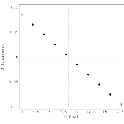
Figure 3: Zeros of $t^{\infty}(U)$ (see equation (18) below) with parameter values $A=1,~{}B=2.5,~{}U_{c}=8.5,~{}\gamma=.01$.

3.1 The Blaschke terms

Let us explain the ”Blaschke-terms”. These arise if the well-known Kramers-Kronig (KK) relations are applied to the logarithm of a regular function $t^{QD}(U)$ of its argument $U$, rather than to $t^{QD}(U)$ itself, as is usual. Then the zeros of $t^{QD}(U)$ add singularities to the KK integrand and these have to be subtracted in a manner that does not affect adversely the conditions that are the basis of the KK relations. As a consequence (for real values of U) one can express the argument (phase) of this function as

$$arg~{}t^{QD}(U)=-\frac{1}{\pi}P\int^{\infty}_{-\infty}\frac{dU^{\prime}}{U^{\prime}-U}ln|t^{QD}(U^{\prime})|+\Phi_{B}(U)$$ (14)

where $P$ represents the principal part of the singular integral and $\Phi_{B}(U)$ is the Blaschke-phase given as the sum of terms

$$\Phi_{B}(U)=-i\sum_{j}ln\frac{U-U^{j}}{U-U^{j*}}$$ (15)

[38]-[39]. Here $U^{j}$ are those zeros of $t^{QD}(U)$ that lie in the upper half of the complex $U$-plane and $U^{j*}$ are their complex conjugates. (Actually, equation (15) can be generalized for poles and branch-points in the upper half-plane by suitably attaching (negative and fractional) weights to each term in the sum, but since we shall find that there are no poles or branch-points in the transmission amplitude for the range of interest, we can disregard these possibilities.)

Now if we look at the integral term, we see that it tends to $0$ for both $U\to-\infty$ and $U\to\infty$ (provided the log-function has no singularities on the real $U$-axis). Therefore, as claimed, this term cannot cause a net gain of the phase, only some structure. Such structure will indeed occur when $|t^{QD}(U)|$ becomes small at some value of $U$. It will have the form of a very sharp peak whenever a zero of $t^{QD}(U)$ will be very close to the real axis. This will occur when $\gamma$ is very small compared to the level spacing, as in equation (12) , for which the level spacing was unity.

A different story are the terms in the Blaschke-phase. Each term will cause a step of $2\pi$ in the phase.

In the enclosed drawings we show $|t^{QD}(U)|$ and $\frac{1}{\pi}arg~{}t^{QD}(U)$ both vs (the real part of) $U$ on the same graph. In the visibility $|t^{QD}(U)|$ one sees the peak structure and in the phase: the initial steps (up to $U=8$), followed (for $U$ above this value) by the rise and lapse of the phases.

4 A Compact Form of the Transmission Amplitude

We now rewrite the preceding expression for the total transmission matrix $t^{QD}(U)$ (making only an approximation that will turn out to have almost no effect on the results) and obtain a compact, closed expression. From this we can deduce the relevant analytic properties of $t^{QD}(U)$ almost by inspection.

Because we expect that for a given value of $U$ only a few (nearly resonant) terms in equation (10) will contribute, we extend the sum in equation (9) to $-\infty$ and $\infty$. The resulting series can be summed to take a simple form

$$\frac{t^{\infty}(U)}{t^{\infty}(U\rightarrow-\infty)}=\frac{1+Ae^{-2\pi i(U-U_{c})/(1-i\gamma)}}{1-B~{}e^{-2\pi i(U-U_{c})/(1-i\gamma)}}$$ (16)

The algebra is based on the result [40]

$$\frac{1}{e^{z}-1}=-\frac{1}{2}+\sum_{n=-\infty}^{\infty}\frac{1}{z-2n\pi i}$$ (17)

from which follows the expansion of $t^{\infty}(U)$ as the series:

$$\frac{t^{\infty}(U)}{t^{\infty}(U\rightarrow-\infty)}=\frac{1}{2}(1-\frac{A}{B})-i(1+\frac{A}{B})\frac{(1-i\gamma)}{2\pi}$$

$$\cdot\sum_{n=-\infty}^{\infty}\frac{1}{U-n-(U_{c}+\frac{\gamma}{2\pi}\ln~{}B)+i(\gamma~{}n+\frac{1}{2\pi}\ln~{}B)}$$ (18)

Recalling now from equation (9) $t^{QD}(U)=t_{h}^{QD}+t_{l}^{QD}(U)$, and noting the expression for $t_{l}^{QD}$ in equation (10) , we can make the following replacements:

$$t_{h}^{QD}=\frac{t^{\infty}(U\rightarrow-\infty)}{2}(1-\frac{A}{B}),\qquad 2\pi G\simeq t^{\infty}(U\rightarrow-\infty)(1+\frac{A}{B})$$

$$R^{\prime}=-U_{c}-\frac{\gamma}{\pi}\ln~{}B,\qquad R"=-\gamma~{}n-\frac{1}{2\pi}\ln~{}B$$ (19)

(In the second equation we have neglected the small and unimportant quantity $-i\gamma$ before the sum.) Equation (19) will lead to the following proportion between $A$ and $B$:

$$\frac{A}{B}=\frac{\pi G-t_{h}^{QD}}{\pi G+t_{h}^{QD}}$$ (20)

The following values of the four parameters ($A,B,U_{c},\gamma$) in the function $t^{QD}(U)$ are compatible with the choices of the parameter in equation (12) .

$$A=1,~{}B=2.5,~{}U_{c}=8.5,~{}\gamma=.0086$$ (21)

The plotted $t^{\infty}(U)$ with these parameters is shown in Fig. 4. The result is virtually identical with that obtained for $t^{QD}(U)$ from the restricted sum in equation (7) , in the gap voltage range of figures 1 and 2. As already noted, the reason is that the contributions to the infinite sum outside the restricted range are negligible. The signal advantage of the compact form in equation (16) , over the partial sum in equation (7) , is that the zeros and poles of the transmission amplitude can be derived from the former considerably simpler. We now obtain these zeros and poles, with the parameters chosen in equation (21) .

4.1 Analysis of zeros and poles

1)  Zeros of equation (16) : These occur when the second term in the numerator is -1, so that

$$U = U_{c}+n+\frac{1}{2}-\frac{\gamma lnA}{2\pi}-i\gamma[(n+\frac{1}{2})+\frac{lnA}{2\gamma\pi}]~{}~{}(n=0~{}or~{}a~{}signed~{}integer)$$ (22)

$$= 8.5+(n+\frac{1}{2})-0.0086i(n+\frac{1}{2})$$

$$= V_{p}(n)+0.0086i[8.5-V_{p}(n)]$$

where in the second line we have inserted the parameter values from equation (21) and in the third line we have written $V_{p}(n)$ for the real part of the $n$’th zero. For a small value of the decay rate $\gamma$ this will be the value of the observed gap voltage at the position of the minimum. It is now apparent that for minima at gap voltages below $8.5$ the zeros will be at positive imaginary parts of $U$, while for gap voltages above $8.5$ the imaginary part will be negative. (This was shown in Fig. 3.)

2) Poles of equation (16) : For these the second term in the denominator must be 1, giving

$$U = U_{c}+m-\frac{\gamma lnB}{2\pi}-i\gamma(m+\frac{lnB}{2\gamma\pi})~{}(m=0~{}or~{}a~{}signed~{}integer)$$ (23)

$$= 8.5+m-0.0086i(m+17)$$

$$= W_{p}(m)-0.0086i[W_{p}(m)+8.5]$$

where again (in the second line) we have substituted the parameters and then have rewritten the equation in terms of the observational gap voltages $W_{p}(n)$ at the maxima. (The small quantity $\frac{\gamma lnB}{2\pi}\approx 0.001$ has been neglected.) It is now clear that the poles lie in the lower half of the $U$-plane for all gap voltages above $-8.5$. Gap voltages below this value are outside the range of interest for the discussion of the experiments.

4.2 Deductions from the compact form

The essential features of this form are that for values of the gate voltage $U$ that are experimentally measured

(1) there are no singularities (i.e., denominator zeros) in the upper complex-$U$ half plane, and

(2) for $ReU>U_{c}$ the zeros of $t^{QD}(U)$ are only in the lower-half of the complex $U$-plane (this is the phase-lapse regime, identified with the integral part in the analytical expression for the phase), whereas for $ReU<U_{c}$ there are zeros in the upper-half of the complex $U$-plane (this is the increasing-phase regime, identified with the Blaschke phase terms). Important in equation (16) are the parameter $U_{c}(=8.5)$ and that $B(=2.5)>A(=1)$. The latter requirement removes the poles from the wrong half-plane and, by equation (20) , translates immediately to the physical requirement that the high lying (Fano-like) states’ transmission amplitude $t^{QD}_{h}$ is real and positive.

Contrasting to our zeros, which are complex, the zeros that were found both in [23] and in [15] were real. In the last work it was indeed pointed out (on p. 106602-4) that the reality was due to the time reversal invariance of the Hamiltonian , tied to an infinitely sharp $\pi$ phase jump, whereas a finite width phase jump could be achieved by inter-level thermal excitation. Alternatively, it could be obtained with a nonzero $\gamma$ due to inelastic electron-phonon interactions, which is the possibility envisaged here, and $B/A>1$ and which, by equation (20) , is contingent to the virtual excitation to meta-stable states.

(At this stage one may want to compare the functions of Table II and the figures in the earlier paper [28] by the present authors, in which the decay parameter $\gamma$ was $0$. A more significant difference is that in the functions of [28] the assumed regions of analyticity were the opposite to that in the present article. The former choice is the natural one if $U$ is identified with a ”time-like” variable, whereas the present choice is the proper one if $U$ is energy or frequency like.)

Figure 4: Visibility amplitude ratio (thick line, arbitrary units) and phase (thin line in radians) as function of gap voltage $ReU$. $|t^{\infty}(U)|$ and arg$~{}t^{\infty}(U)$ are plotted from equation (16) with parameter values $A=1,~{}B=2.5,~{}U_{c}=8.5,~{}\gamma=.0086$.

Changes in some parameters can alter, e.g., the relative magnitudes of the peaks. The slope of the phase-lapse in the figure is proportional to the height of the minima in the visibility above the origin. (This property was first predicted in [28] and rediscovered in several subsequent papers.)

4.3 A remark on the phase-step magnitude

The phase shown in the drawing for the initial (step-up) regime is not the same as in e.g. [5] or [8], in that we predict a net phase gain of $2\pi$ per peak, whereas the experimental phase steps seem (in most cases) to be less than this. If the discrepancy really exists, the present interpretation may have to be withdrawn or be changed in a way not clear to us just now. However, it seems that the experimental phases are not traced quite precisely throughout the step. Thus, when the visibility is near zero, the phase changes may not be properly recorded, but rather sawn together in a continuous fashion so that part of the rise is lost.

5 Speculating on the Decay Mechanism: Electron-LO Phonon Coupling ?

Assuming a ladder-like structure for the low lying electronic levels in the quantum dot, with level separation of unity (when expressed in the units of $U$), our expression for $t^{\infty}(U)$ with $A=0$ can be simply understood as the Green function of broadened regularly spaced electronic states. The pre-exponential factor $B$ and the $i\gamma$ part in the exponent then represent the broadening of low lying levels. Were the former 1 and the latter 0, we would have the Green function for a series of equidistant, infinitely sharp electronic levels. However, our main interest is in the zeros of the numerator. These arise because $A\neq 0$.

The phonon-bottleneck or its absence has long been under consideration for the mechanism of decay of discrete electronic levels in quantum dots [31]-[34]. It is generally supposed that LO phonons in the dot of energy $\hbar\omega_{LO}$ couple to the levels. It has also been noted that when the electron level structure at some rung in the ladder gets into near coincidence with the phonon energy, then a Rabi splitting takes place. The physical meaning of this is that the near-coincidental excited electron-level gets strongly admixed with the ground electronic level in which one LO phonon is excited. As a result, two admixture levels are formed, which are separated by roughly the coupling energy between the electron and the LO phonon. The condition for coincidence to occur at the $n_{R}$ (R for Rabi) electronic level is that

$$n_{R}\Delta\approx\hbar\omega_{LO}$$ (24)

where $\Delta$ is the electronic energy separation.

We speculate that the decay in $t^{QD}(U)$ reflects this resonance condition i.e. $\hbar\omega_{LO}=n_{R}\Delta\approx N_{lowlying}\Delta$, since above the low lying levels commences the LO -phonon decay mechanism. We have not calculated the transmission matrix of the coupled electron-LO optical excitation (constituting a polaron), along the lines of [41]-[44]. With the estimates of [14] that $\Delta=40\mu eV$ (which may be a minimal estimate) and that there are $N_{lowlying}\approx 200$ electronic states up to the brim of the quantum dot well, one obtains $8meV$ for the height of electronic levels, at which the phonon coupling causes an effective admixture. This is about a quarter (of $\hbar\omega_{LO}=36meV$) where we would expect the electron-phonon coupling to be felt in GaAs [34]. Our computations have stopped at $N_{lowlying}=34$, since the experimental range of scanned levels is considerably below this. No observable difference would be felt by extending the sum to $N_{lowlying}$ placed in the hundreds.

6 Conclusion

The two distinct regimes in the electron-transmission phase of an Aharonov-Bohm arrangement containing a quantum dot, already present in earlier experiments in [3]-[7] but recently definitively established in [8], have been explained by a model based on a ladder of electronic levels with increasingly faster decay from higher levels up to a meta-stable continuum (or bunch of Fano-type levels) with very short life-times. The decay mechanism is tentatively surmised as due to LO phonons in the dot. Though a Hamiltonian is postulated, its implementation in the transmission amplitude is phenomenological.

Among the main new features of this work, not present in several previous theories, are the postulate of the large widths of Fano-type states that are above the quantum well, the treatment of geometrical effects (side-arms in the ring) on the same footing as the admixture with meta-stable states to disrupt the unitarity [23], and the finding that at least three particle states are needed to reproduce the observed phase behavior. In formal terms, the two regimes of phases, increasing across the resonance and those returning to former values are identified with zeros (but not the poles!) of the complex transmission lying (respectively) in the lower and upper half planes of the complex energy (or gap voltage) variable. The absence of poles is connected to the meta-stable state, but the zeros do not arise from the usual Fano-form or from cancellation between adjacent resonances.

Acknowledgements

We thank Amnon Aharony, Yuval Gefen and Yuval Oreg for valuable remarks on our work and the first for suggestions.

References

- [1] 9
- [2] Y. Gefen, Y. Imry and M. Ya. Azbel, Phys. Rev. Lett. 52 128 (1984)
- [3] A. Yacobi , M. Heiblum, D. Mahalu and H. Shtrikman, Phys. Rev. Lett. 744047 (1995) A. Yacobi, H. Shtrikman and M. Heiblum, Phys. Rev. B 53 9583 (1996)
- [4] E. Buks, R. Schuster, M. Heiblum, V. Umansky and H. Shtrikman, Phys. Rev. Lett. 77 4664 (1996)
- [5] R. Schuster, E. Buks, M. Heiblum, D. Mahalu, V. Umansky and H. Shtrikman, Nature 385 417 (1997)
- [6] Y. Ji, M. Heilblum, D. Sprinzak, D. Mahalu and H. Shtrikman, Science 290 779 (2000)
- [7] Y. Ji, M. Heilblum and H. Shtrikman, Phys. Rev. Lett. 66 076601 (2002)
- [8] M. Avinun-Kalish, M. Heiblum, O. Zarchin, D. Mahalu and V. Umansky, Nature 436 529 (2005)
- [9] K. Kobayashi, H. Aikawa, S Katsumoto and Y. Iye, Phys. Rev. Lett. 88 256806 (2002); H. Aikawa, K. Kobayashi, A. Sano, S. Katsumoto and Y. Iye, cond-mat /0309084 (3 Sept. 2003)
- [10] Y. Oreg and Y. Gefen , Phys. Rev. B 55 13726 (1997)
- [11] G.Hackenbroich and H.A. Weidenmüller, Phys. Rev. Lett. 76, 110 (1996); Phys. Rev. B 53 16 379 (1996); Europhys. Lett. 38 129 (1997)
- [12] H. Xu and W. Sheng, Phys. Rev. B 57 11903 (1998)
- [13] C.-M. Ryu and Y.S. Cho, Phys. Rev. B 58 3572 (1998)
- [14] G. Hackenbroich, Phys. Rep. 343 463 (2001)
- [15] P.G. Silvestrov and Y. Imry, Phys. Rev. Lett. 85 2565 (2000);Phys. Rev. Lett. 90106602 (2003)
- [16] O. Entin-Wohlman, A. Aharony and V. Kashcheyevs, J. Phys. Soc. Japan (Suppl. A)72 77 (2003)
- [17] A. Aharony, O. Entin-Wohlman, B.I. Halperin and Y. Imry, Phys. Rev. B 66 115311 (2002)
- [18] A. Silva, Y. Oreg and Y. Gefen, Phys. Rev. B 66 195316 (2002)
- [19] D.I. Golosov and Y. Gefen, cond-mat /0601342 (16 January 2006)
- [20] A. Jerez, P. Vitushinsky and M. Lavagna, Phys. Rev. Lett. 95 127203 (2005)
- [21] P.J. Price, Phys. Rev. B 38 1994 (1988); IEEE Trans. Electron. Devices 39520 (1992)
- [22] W. Porod, Z. Shao and C.S. Lent, Phys. Rev. B 48 8495 (1993)
- [23] Z. Shao, W. Porod and C.S. Lent, Phys. Rev. B 49 7453 (1994)
- [24] U. Fano, Phys. Rev. 124 1866 (1961)
- [25] O. Entin-Wohlman, A. Aharony, Y. Imry amd Y. Levinson, J. Low Temp. Phys. 126 1251 (2002)
- [26] P.S. Deo, Physica E 1 301 (1997); Solid State Commun. 107 69 (1998)
- [27] ”Expected ’mesoscopic’ features in the phase, related to the dot’s shape, spin degeneracy or to exchange effects, were never observed. Presently, there is no satisfactory explanation for the observed phase ’universality’.” (Taken from the opening paragraph of [8].)
- [28] R. Englman and A. Yahalom, Phys. Rev. B 61 2716 (2000)
- [29] G. Baym Lectures on Quantum Mechanics (Benjamin, New York, 1969) pp. 104-113
- [30] K. Hirose, Y. Meir and N.S. Wingren, Phys.Rev.Lett. 90 026804 (2003)
- [31] B. Beckelmann and G. Bastard, Phys. Rev. B 42 8947 (1990)
- [32] X.Q. Li, H. Nakayama and Y. Arakawa, Phys. Rev. B 59 5069 (1999)
- [33] T. Inoshita and H. Sasaki, Physica B 227 373 (1996); Phys. Rev. B 56 R4355 (1997)
- [34] T. Stauber, R. Zimmermann and H. Castella, Phys. Rev. B 62 7336 (2000)
- [35] R. Baltin and Y. Gefen, Phys. Rev. Lett. 83 5094 (1999)
- [36] R. A. E. C. Paley and N. Wiener, Fourier Transforms in the Complex Domain (American Physical Society, New York,1934) p.15, Theorem XII
- [37] E.C. Titchmarsh, Introduction to the Theory of Fourier Integrals (Clarendon Press, Oxford, 1948) Chap. V
- [38] N.G. van Kampen, Phys. Rev. 89 1072 (1953)
- [39] L. Mandel and E. Wolf, Coherence and Quantum Optics (University Press, Cambridge, 1995) section 7.3.2
- [40] T.A. MacRobert, Functions of a Complex Variable ( MacMillan, London, 1938) p.128
- [41] L. I. Glazman and R.I. Shekhter, Sov. Pys. LETP, 67 163 (1988)
- [42] A.-P. Jauho, N.S. Wingreen and Y. Meir, Phys. Rev. B 50 5528 (1994)
- [43] O. Entin-Wohlman, Y. Imry and A. Aharony, Phys. Rev. Lett. 91 046802 (2003)
- [44] P. Machnikowski and L. Jacak, Phys. Rev. B 71115309 (2005)