Boundary field induced first order transition in the 2D Ising model: Exact study

Abstract

We present in this article an exact study of a first order transition induced by an inhomogeneous boundary magnetic field in the 2D Ising model. From a previous analysis of the interfacial free energy in the discrete case (J. Phys. A: Math. Gen.38, 2849, 2005) we identify, using an asymptotic expansion in the thermodynamic limit, the line of transition that separates the regime where the interface is localised near the boundary from the one where it is propagating inside the bulk. In particular, the critical line has a strong dependence on the aspect ratio of the lattice.

1 Introduction

The 2D Ising model is certainly one of the most famous statistical models in physics with connections in various fields of research. Despite its apparent simplicity, it contains generic properties for phase transitions. From the interpretation of the Ising model as a lattice gas model, it was used as a simple model for wetting transitions. A number of theoretical and numerical tools have been developed to study such transitions. One of the first steps comes from McCoy and Wu who developed the theory of Toeplitz determinants [1] in order to solve the 2D Ising model with uniform boundary magnetic field (see also [2, 3, 4]. Surface fields can be considered as the effect of boundary impurities or constraints that change the properties of bulk spins. They also can be viewed as a chemical potential difference between the bulk and the wall of the system in a binary mixture. The wall can indeed attract one species more than the other, leading so to an effective field [5]. A major contribution is due to D.B. Abraham in the early 80’s who developed efficient methods [6] based on transfer matrix techniques in order to solve the 2D Ising model with various fixed boundary conditions (the spins are constraint to be up or down on the boundary according to different profiles of the boundary spins). Theses techniques allow the computation of the surface tension energy for different profiles of the boundary conditions. Important questions arise whether the interface between two phases and produced by boundary impurities is diffuse or sharp (see discussion in [7]) and how it diverges with the system size. These questions are closely related in general to the existence of roughening transitions in such systems close to the bulk critical temperature. A generalisation of McCoy and Wu result for the uniform boundary field case is to take two opposite surface fields $H_{1}$ and $H_{2}$ on a Ising strip, where a domain wall propagates in the middle of the strip when the fields have opposite signs [7, 8, 9]. A wetting temperature $T_{\mathrm{w}}(H_{1},H_{2})$ occurs at slightly below the bulk temperature $T_{\mathrm{c}}$ where a well defined interface appears in the middle of the strip. This temperature can also be defined as the transition between diffuse and sharp interfacial regimes. In the particular case of an infinite strip, the width of the strip is only important for the magnetisation profile and for the scaling of the typical length of the interface extension [9, 10, 11, 12], which diverges typically like the inverse of $(T-T_{\mathrm{w}})$ above $T_{\mathrm{w}}$, giving an interface correlation length exponent equal to unity. Technically, a generic way to implement a finite boundary magnetic field from an infinite one is to take the bonds perpendicular to the surface field line a fraction of the bulk bonds. For example if the spins subject to an infinite magnetic field $H_{1}=\pm\infty$ and located along the surface are noted $\sigma_{1,n}$, $n=1\dots L_{y}$, and if the bulk coupling is $J$, taking $J_{0}$ as the coupling between $\sigma_{1,n}$ and $\sigma_{2,n}$ generates on spins $\sigma_{2,n}$ a field proportional to $\pm J_{0}/J$. The value of this field can then be tuned by varying $J_{0}$, and this specificity is discussed in several publications [7, 12, 13]. In these different cases, the way the thermodynamic limit is taken is also important.
The effect of an inhomogeneous magnetic field on one border is therefore an interesting problem because it generates a localised interface whose extension inside the bulk can be studied in the framework of diffusion processes. In particular the interface generated by two opposite magnetic fields of infinite amplitude in the critical Ising model is a typical example of Schramm-Loewner evolutions (SLE) [14]. It is generally restricted to the conditions of infinite strip models, and the typical size of the interface is scaled with the strip width. In this paper we want to focus on another particular geometry that can be treated exactly, where we apply a non homogeneous surface field on a rectangular Ising lattice. We will see that the interfacial free energy can be evaluated in the discrete case and that, in the thermodynamic limit, two dominant and competing terms determine whether the interface stays localised on the surface or is extended inside the bulk, depending on the lattice aspect ratio. This model, even if the perturbation stays on the surface, shows some interesting complexity in the bulk. The techniques used here are based on Grassmann variables [15, 16, 17, 18, 19, 20] and can interestingly be extended to other configurations as well. Experimentally it might be important to take account of the geometry of the system like the ratio of typical length scales to determine the values of the critical field or temperature, as we are going to see in the following.
This article is organised as follow: We summarise in section 2 a previous exact result in the discrete case of the free energy contribution due to a inhomogeneous magnetic field. The analytical expression is however not easy to deal with and is rather obscure from a physical point of view, even if it has the advantage to prevent the use of any cut-off, inherent to continuous models. Simple arguments for the formation of the bulk interface as function of field amplitude are given at zero temperature. An asymptotic method to obtain the thermodynamic limit of the discrete solution is presented in section 3, and show the simple effect of the system size ratio on the transition line. Monte Carlo simulations are also used to confirm the phase diagram. We then conclude and propose briefly the possibility of extensions of our method to other surface effects.

2 The model

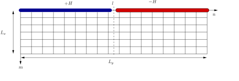
Figure 1: Inhomogeneous field configuration on the lattice. The field is positive for the sites $(m,n)=(1,1)\dots(1,L_{y}/2)$ and negative on the rest of the line. Periodic conditions are imposed along the $y$-direction, and open conditions on the transverse direction.

We consider in this paper a finite 2D Ising system with a non homogeneous magnetic field $h_{n}$ located on one boundary of the system. This system is periodic along the $y$-direction, see figure 1, and with open boundaries for the transverse $x$-direction, one of the latter boundaries being under a magnetic field. The Hamiltonian is simply given by

$$\mathcal{H}=-J\sum_{m,n=1}^{L_{x},L_{y}}(\sigma_{mn}\sigma_{m+1n}+\sigma_{mn}\sigma_{mn+1})-\sum_{n=1}^{L_{y}}h_{n}\sigma_{1n},$$ (1)

with $\sigma_{m1}=\sigma_{mL_{y}+1}$ and $\sigma_{0n}=\sigma_{L_{x}+1n}=0$. The notations are the same as in a previous publication [20] where an exact expression for the free energy in the case of finite size and discrete lattice case was obtained using Grassmann techniques and Plechko method based on Grassmann operator ordering [15, 16]. These operators replace basically spin operators, and in the 2D case, they lead to a Grassmannian quadratic action which is exactly solvable in the Fourier space. We have found in particular an exact ordering of border operators associated with a general boundary magnetic field and then obtained, after integration over bulk degrees of freedom, a quadratic 1D action with effective Grassmannian magnetic fields (see equation (61) in reference [20]), for equal system sizes $L_{x}=L_{y}$. This 1D action represents the free energy contribution from the boundary fields. The case with different sizes $L_{x}\neq L_{y}$ is easily implemented as we will see below. As an application, we have considered in [20] the interface initiated by an inhomogeneous magnetic field of configuration shown in figure 1, with $h_{n}=H$ for $n=1\dots L_{y}/2$ and $h_{n}=-H$ for $n=L_{y}/2+1\dots L_{y}$. Computing the interface energy $\sigma_{\mathrm{int}}$ in the inhomogeneous case is equivalent to solve a set of Grassmannian two points correlation functions (see equation (74) in [20]) using the previous 1D boundary action for the homogeneous case, which is done exactly. For more general configurations, with different sequences of fields $(H_{k};l_{k})$, i.e. $h_{n}=H_{k}$ for $n=l_{k}+1\dots l_{k+1}$, the problem is treated identically [20]. In this paper, we will consider the solution for the interface energy (see equation (84) in [20] and below), with $L_{x}\neq L_{y}$, and study the thermodynamic limit with fixed aspect ratio $\zeta=L_{x}/L_{y}$. Numerically, the difficulty to compute this free energy arises from the fact that it is expressed as the logarithm of some argument which is an exponential small number in the system size, especially at low temperature. Moreover, to study in detail the phase transition corresponding to the propagation of the interface from where the magnetic field changes its sign, we need to take directly the thermodynamic limit, and the purpose of this paper is precisely to study how the discrete expression of the interface energy behaves when we take the limits $L_{x},L_{y}\rightarrow\infty$.

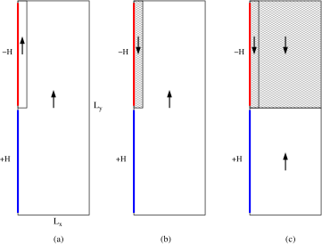
Figure 2: Spins configurations at $T=0$ under various conditions: (a) $L_{x}/L_{y}>\zeta_{\mathrm{s}}$, $H<J(1+4/L_{y})$, (b) $L_{x}/L_{y}>\zeta_{\mathrm{s}}$, $H>J(1+4/L_{y})$ and (c), $L_{x}/L_{y}<\zeta_{\mathrm{s}}$, $H>H_{\mathrm{s}}=4JL_{x}/L_{y}$.

The presence of an interface phase transition at zero temperature can be analysed with simple energetic arguments. For small values of the field $H$, all spins are pointing in the same direction, say up, because boundary negative fields are not strong enough to compete with transverse Ising couplings and reverse the corresponding spins (see figure 2a). The energy in this case is $E_{0}$. When increasing the field, the spins $\sigma_{L_{y}/2+1,1}\dots\sigma_{L_{y},1}$ will eventually reverse their sign, and the corresponding energy is $E_{1}=E_{0}-HL_{y}+2J(L_{y}/2+2)$, which is lower than $E_{0}$ if $H>J(1+4/L_{y})$ (see figure 2b). Another possible configuration is when all spins $\sigma_{L_{y}/2+1,j}\dots\sigma_{L_{y},j}$, for $j=1\dots L_{x}$, reverse their sign (see figure 2c). In this case, the total magnetisation is zero, and the corresponding energy is $E_{2}=E_{0}-HL_{y}+4JL_{x}$, which is lower than $E_{0}$ for $H>4\zeta J$. Comparing the energies $E_{1}$ and $E_{2}$, we conclude that the interface stays on the boundary if $\zeta>1/4+1/L_{y}=\zeta_{\mathrm{s}}$ ($E_{1}<E_{2}$, and $H>J(1+4/L_{y})$), and propagates inside the bulk when $\zeta$ is smaller than the critical ratio value $\zeta_{\mathrm{s}}$ and $H$ larger than $H_{\mathrm{s}}\equiv 4\zeta J$. In the latter case, where the total bulk magnetisation spontaneously goes from unity to zero, the transition is first order.
In the thermodynamic limit, $\zeta_{\mathrm{s}}$ tends to $1/4$. This particular value is actually deeply related to the boundary condition in the $y$-direction. For free boundary conditions we would have found $\zeta_{\mathrm{s}}=1/2$ instead. The physical interpretation of this threshold is simplified by the study of boundary spin-spin correlation function for various $\zeta$. A direct extension of results in [20] leads to the figure 3. For $L_{x}\ll L_{y}$ we observe an exponential decay of the correlation functions, typical of a 1D behaviour. If the aspect ratio increases, we observe a obvious crossover towards a 2D behaviour at large $\zeta$. The crossover is obtained in this case for $\zeta\simeq 1/4$.
In particular, we would like to know in the following how the transition line $H_{\mathrm{s}}(T)$ for $\zeta<1/4$ behaves as the temperature is increased to near the second order phase transition at $T_{\mathrm{c}}/J=1/\tanh^{-1}(\sqrt{2}-1)\simeq 2.27$.

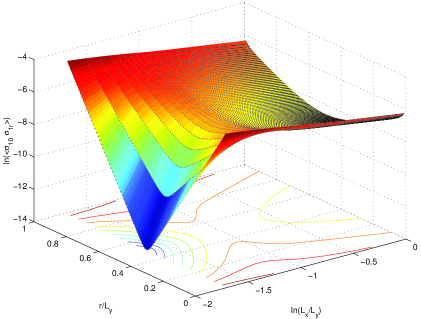
Figure 3: Boundary spin-spin correlation function $\langle\sigma_{10}\sigma_{1r}\rangle$ as a function of $r/L_{y}$ and aspect ratio $\zeta=L_{x}/L_{y}$, at $T=2J$, $H=0.1J$ and for $L_{y}=100$. Note the crossover from a 1D behaviour to a 2D behaviour at $\zeta\simeq 1/4$.

3 Analysis of the thermodynamic limit

The Hamiltonian (1) leads to the decomposition of the total free energy ${\cal F}$ as follows:

$${\cal F}(T,H)={\cal F}_{0}(T,H)+{\cal F}_{\mathrm{hom}}(T,H)+\sigma_{\mathrm{int}}(T,H),$$

where ${\cal F}_{0}$ is the free energy in zero field, ${\cal F}_{\mathrm{hom}}$ the additional free energy corresponding to an homogeneous boundary magnetic field $H$. The contribution $\sigma_{\mathrm{int}}$ is the corrective term due to the change of sign of boundary magnetic field. The exact expressions for those terms in the discrete case can be found in [20]. As $\sigma_{\mathrm{int}}$ is the only term corresponding to inhomogeneous surface conditions, it contains all the physical informations about the transition described in the previous section. The section (3.1) starts with the calculation of $\sigma_{\mathrm{int}}$ in the thermodynamic limit and the evaluation of finite size corrections as well. This allows us to characterize the details of the transition: In section (3.2), we obtain the expression of the transition line and the corresponding phase diagram, and in section (3.3) we analyse the behaviour of this line at low temperature and close to the bulk critical point. Finally, in section (3.4), we summarize the different results and the physical interpretation.

3.1 Expression of the interfacial free energy

We start with the discrete expression of the boundary free energy $\sigma_{\mathrm{int}}$ taken from reference [20] (see equation (84) in that paper). It was obtained by computing two point correlation functions with a Grassmannian quadratic action expressed in Fourier modes. The corresponding result is the following:

$$-\beta\sigma_{\mathrm{int}}=\log\left[1-\frac{2}{L_{y}}\sum_{q=0}^{L_{y}/2-1}(-1)^{q}\cot(\theta_{q+\frac{1}{2}}/2)F(\cos\theta_{q+\frac{1}{2}})\right],$$ (2)

where $\theta_{q}=(2\pi/L_{y})(q+1/2)$, and $F$ is a function of $t=\tanh\beta J$ and $u=\tanh\beta H$ defined as

$$F(x) = \frac{4tu^{2}G(x)}{\frac{1}{4}[1-(1+t^{2})(t^{2}+2tx-1)G(x)]^{2}+2tu^{2}(1+x)G(x)+4t^{4}(1-x^{2})G(x)^{2}}.$$ (3)

The function $G$ is defined by

$$G(x) = \frac{1}{L_{x}}\sum_{p=0}^{Lx-1}\frac{1}{(1+t^{2})^{2}-2t(1-t^{2})(\cos\theta_{p}+x)},$$ (4)

where $\theta_{p}=2\pi p/L_{x}$. We propose in this section to simplify the expression (2) by studying the thermodynamic limit, in order to obtain the dominant terms contributing to the free energy. The sum inside the logarithm function (2) has the particularity to behave like a Dirac distribution in the limit $L_{y}\rightarrow\infty$. Indeed, we define first the following sum

$$S[F]=\frac{2}{L_{y}}\sum_{q=0}^{L_{y}/2-1}(-1)^{q}\cot(\theta_{q+\frac{1}{2}}/2)F(\cos(\theta_{q+\frac{1}{2}})),$$ (5)

for any function $F$. In A, we demonstrate that in the thermodynamic limit, this sum is simply $F(1)$, plus corrections which are exponentially small in the system size $L_{y}$. These corrections are important for finding the asymptotic behaviour of the interface free energy. We are expecting $\sigma_{\mathrm{int}}$ to be linear in $L_{x}$ or $L_{y}$, so the argument in the logarithm (2) should be exponentially small in $L_{x}$ or $L_{y}$. In particular, the $L_{y}$ dependence is contained in the corrections of the Dirac distribution, and the $L_{x}$ dependence is contained in the term $F(1)$ through the finite sum $G$, equation (4). From A and equation (33), we can expand $S[F]$ in the limit of large $L_{y}$ and we obtain for the dominant part

$$S[F]\simeq F(1)-A_{L_{y}/2},$$ (6)

where $A_{L_{y}/2}$ is the $L_{y}/2$-th Fourier coefficient of the function $F$, and it will be shown that it goes to zero exponentially in $L_{y}$. The term $F(1)$ is equal to

$$F(1)=\frac{4tu^{2}G(1)}{[1-(1+t^{2})(t^{2}+2t-1)G(1)]^{2}/4+4tu^{2}G(1)},$$

and $G(1)$ given by (4) can be expanded as a Fourier series the following way

$$G(1)=\frac{1}{L_{x}}\sum_{p=0}^{Lx}\sum_{k\geq 0}B_{k}\cos(k\theta_{p}),$$ (7)

where the Fourier coefficients $B_{k}$ are defined by

$$B_{0} = \frac{1}{2\pi}\int_{0}^{2\pi}\mathrm{d}\theta\frac{1}{(1+t^{2})^{2}-2t(1-t^{2})(1+\cos\theta)},$$ (8)

$$B_{k>0} = \frac{1}{\pi}\int_{0}^{2\pi}\mathrm{d}\theta\frac{\cos(k\theta)}{(1+t^{2})^{2}-2t(1-t^{2})(1+\cos\theta)}.$$

Using

$$\frac{1}{2\pi}\int_{0}^{2\pi}\frac{\mathrm{d}\theta}{a-b\cos\theta}=\frac{1}{\sqrt{a^{2}-b^{2}}},$$ (9)

we arrive at the expression $B_{0}=1/[(1+t^{2})|t^{2}+2t-1|]$. It is then easy to show that

$$G(1)=\sum_{k\geq 0}B_{k}\frac{1}{L_{x}}\sum_{p=0}^{L_{x}-1}\cos(k\theta_{p})=B_{0}+B_{L_{x}}+B_{2L_{x}}+\dots$$ (10)

We expand then $F(1)$ for $L_{x}$ large, when $B_{L_{x}}$ is small, and it is sufficient to keep the first two terms:

$$F(1) \simeq \frac{4tu^{2}(B_{0}+B_{L_{x}})}{\frac{1}{4}[1-(1+t^{2})(t^{2}+2t-1)(B_{0}+B_{L_{x}})]^{2}+4tu^{2}(B_{0}+B_{L_{x}})},$$ (11)

$$\simeq 1-\frac{(1+t^{2})^{2}(t^{2}+2t-1)^{2}}{16tu^{2}}\frac{B_{L_{x}}^{2}}{B_{0}}.$$

We have check that the coefficient $B_{2L_{x}}$, which would be of the order of $B_{L_{x}}^{2}$, does not appear at this order. $B_{L_{x}}$ can be computed analytically in the complex plane. If we define $z=\exp(i\theta)$, we have $B_{L_{x}}={\rm Re}\oint\mathrm{d}z/(2i\pi)4z^{L_{x}}/Q(z)$, where $Q(z)$ is a polynomial function

$$Q(z) = -2t(1-t^{2})z^{2}+2z[(1+t^{2})^{2}-2t(1-t^{2})]-2t(1-t^{2}),$$

$$= -2t(1-t^{2})(z-z_{-})(z-z_{+}).$$

The zeros $z_{\pm}$ of this function are distributed on the positive real axis with $z_{-}=(1-t)/[t(1+t)],\;\;z_{+}=1/z_{-}$. $z_{-}$ is less than 1 (or $z_{-}<z_{+}$) for $t>t_{\mathrm{c}}=\sqrt{2}-1$, in the low temperature regime (therefore the quantity $t^{2}+2t-1$ is always positive). The value of $B_{L_{x}}$ in this region is then equal to

$$B_{L_{x}}=\frac{2}{(1+t^{2})(t^{2}+2t-1)}\left(\frac{1-t}{t(1+t)}\right)^{L_{x}}.$$ (13)

We obtain therefore, for the dominant part of the distribution $S$:

$$S[F]\simeq 1-\frac{(1+t^{2})(t^{2}+2t-1)}{4tu^{2}}\left(\frac{1-t}{t(1+t)}\right)^{2L_{x}}-A_{L_{y}/2}.$$ (14)

These corrective terms are all negative, since $1-S[F]$ should be positive so that the logarithm in (2) is always defined, and the interfacial free energy can now be written as

$$-\beta\sigma_{\mathrm{int}} = \log\left(1-S[F]\right),$$ (15)

$$\simeq \log\left(\frac{(1+t^{2})(t^{2}+2t-1)}{4tu^{2}}\left(\frac{1-t}{t(1+t)}\right)^{2L_{x}}+A_{L_{y}/2}\right).$$

The Fourier coefficient $A_{L_{y}/2}$ is evaluated for large $L_{y}$ with the function (3). We expect this coefficient to be exponentially small with $L_{y}$, with some corrections to this coefficient which are also small in $L_{x}$. Therefore the dominant term can be obtained by taking the limit $L_{x}=\infty$ in (4). Using the formula (9) we obtain in this limit

$$G(\cos\theta) = \frac{1}{\sqrt{R(\cos\theta)}},$$ (16)

$$R(\cos\theta) = [(1+t^{2})^{2}+2t(1-t^{2})(1-\cos\theta)][(1+t^{2})^{2}-2t(1-t^{2})(1+\cos\theta)].$$

The function $F$ can then be rewritten, after some algebra, as

$$F(\cos\theta)=\frac{8tu^{2}}{4tu^{2}(1+\cos\theta)+(1+t^{2})(1-2t\cos\theta-t^{2})+\sqrt{R(\cos\theta)}}.$$ (17)

Now $A_{L_{y}/2}$ can be expressed by mean of a complex integration along the unit circle

$$A_{L_{y}/2} = {\rm{Re}}\frac{1}{\pi}\int_{0}^{2\pi}\mathrm{d}\theta F(\cos\theta)\exp\left(i\frac{L_{y}}{2}\theta\right),$$ (18)

$$= {\rm{Re}}\oint\frac{\mathrm{d}z}{2i\pi}F\left(\frac{z^{2}+1}{2z}\right)2z^{L_{y}/2-1}.$$

The value of this integral depends on the poles of the function $F$. Setting $X=(z^{2}+1)/2z$, we can write

$$F(X)=\frac{8tu^{2}}{P(X)+\sqrt{R(X)}}=\frac{8tu^{2}\Big{(}P(X)-\sqrt{R(X)}\Big{)}}{P(X)^{2}-R(X)}.$$ (19)

The polynomial $P(X)^{2}-R(X)$ is a second order polynomial in $X$, and has two zeros which are

$$X_{0}=\frac{1}{2}\frac{2t^{3}-2tu^{4}-u^{2}(1-t^{4})}{t(1-u^{2})(t^{2}-u^{2})},\;\;X_{1}=-1.$$ (20)

$X_{1}$ is not a pole of the function $F$ since it is not a zero of $P(X)+\sqrt{R(X)}$. Indeed, we have $P(-1)+\sqrt{R(-1)}=(1+t^{2})(1+2t-t^{2}+|1+2t-t^{2}|)>0$, because $1+2t-t^{2}$ is always positive in the interval $0<t<1$. Then only $X_{0}$ is pole of $F$, and in the complex plane this gives two solutions $Z_{\pm}$ of the equation $z^{2}-2X_{0}z+1=0$. If $Z_{-}$ is the solution which is inside the unit circle ($|X_{0}|>1$), the value of $A_{L_{y}/2}$ is given by

$$A_{L_{y}/2} = {\rm Re}\left(\frac{P(X_{0})-\sqrt{R(X_{0})})}{(P(X)^{2}-Q(X))^{\prime}(X_{0})\sqrt{X_{0}^{2}-1}}Z_{-}^{L_{y}/2-1}\right),$$

$$\equiv C_{y}(t,u)|Z_{-}|^{L_{y}/2}.$$

In some cases the zeros can be on the unit circle ($|X_{0}|<1$), but we assume this latter situation is not physical since this would mean that the thermodynamic limit is never obtained.
Finally the free energy for the interface in the large system size limit can be written as the logarithm of two dominant terms

$$-\beta\sigma_{\mathrm{int}}\simeq\log\left[\frac{(1+t^{2})(t^{2}+2t-1)}{4tu^{2}}\left(\frac{1-t}{t(1+t)}\right)^{2L_{x}}+C_{y}(t,u)|Z_{-}|^{L_{y}/2}\right].$$ (22)

3.2 Line transition and phase diagram

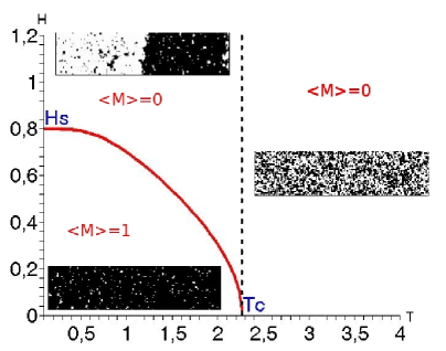
Figure 4: Phase diagram for the system at $\zeta=0.2$. The plain line represents the first order transition given by equation (23). The dashed line is the bulk 2^nd order phase transition. The snapshots are extracted from Monte Carlo simulations in the different regimes, for $L_{x}=40$ and $L_{y}=200$.

Two different regimes can be identified from equation (22), depending on whether the first term in the logarithm is greater or smaller than the second one. In the first case, the free energy is proportional to $L_{x}$ and a coefficient which does not depend on magnetic field, only on $t$. At zero temperature, it is easy to show that $\sigma_{\mathrm{int}}\simeq 4J\zeta L_{y}$, which corresponds to the energy $E_{2}$ computed above in section (2). This means that this term represents a situation where it is energetically favourable for the interface to spread inside the bulk. On the other hand, the second term in the logarithm of equation (22) represents a configuration where the interface is localised on the boundary. Between these two regimes, we can define a line of transition which is a priori first order: The first term does not depend on the magnetic field, therefore the free energy has in general a cusp as a function of $u$) by making the two exponential terms in (22) equal in magnitude.
We then obtain the transition line equation in the $(t,u)$-plane which is simply a quartic polynomial in $u$:

$$2t\Big{(}1+v(4\zeta)\Big{)}u^{4}+(1+t^{2})\Big{(}1-2tv(4\zeta)-t^{2}\Big{)}u^{2}+2\Big{(}v(4\zeta)-1\Big{)}t^{3}=0,$$ (23)

$$v(4\zeta)=\cosh\left[4\zeta\ln\left(\frac{1-t}{t(1+t)}\right)\right].$$

On figure 4 is shown the phase diagram for the system at $\zeta=0.2$, with snapshots of typical configurations at low and large fields/temperatures, obtained by Monte Carlo numerical simulations.

3.3 Behaviour around $T=0$ and $T=T_{c}$

Near zero temperature, we can expand the previous relation with $t=(1-\epsilon)/(1+\epsilon)$, $\epsilon=\exp(-2/T)\ll 1$. We obtain at lowest order in $\epsilon$ and for $4\zeta<1$:

$$(1+2\epsilon^{4\zeta})u^{4}-2u^{2}+1-2\epsilon^{4\zeta}=0,$$ (24)

which gives, $u^{2}=1$ or $u^{2}=(1-2\epsilon^{4\zeta})/(1+2\epsilon^{4\zeta})$. The non trivial solution gives the point $H_{\mathrm{s}}=4\zeta J$ as expected at zero temperature from preliminary study. Moreover, if the transition line ends at the point $u=0$, this is equivalent to $X_{0}=v=1$, or $1-t=t(1+t)$, which gives $t=t_{\mathrm{c}}$. The line ends therefore at the second order transition point. In this case $Z_{+}=Z_{-}=1$, which is the transition value between an exponential behaviour and oscillating one in the logarithm arguments (2). This basically suggests that the interface free energy is no more an extensive function of the system size, and does not contribute to the thermodynamic behaviour of the system. In the case when $4\zeta>1$, the discriminant $\Delta$ of the equation (23) can be written as

$$\Delta = 4t^{2}(1-t^{2})^{2}\left(v-\frac{(1+t^{2})^{2}+2t(1-t^{2})}{2t(1-t^{2})}\right)\left(v-\frac{(1+t^{2})^{2}-2t(1-t^{2})}{2t(1-t^{2})}\right),$$ (25)

$$= 4t^{2}(1-t^{2})^{2}\left(v-\frac{(1+t^{2})^{2}+2t(1-t^{2})}{2t(1-t^{2})}\right)\left(v-v(1)\right).$$

Expanding $v(4\zeta)$ near the threshold value $4\zeta_{\mathrm{s}}=1$, we obtain

$$v(4\zeta)\simeq v(1)+(4\zeta-1)\ln\left[\frac{1-t}{t(1+t)}\right]\sinh\left(\ln\left[\frac{1-t}{t(1+t)}\right]\right),$$

and the discriminant can be expanded as

$$\Delta\simeq 8t^{2}(1-t^{2})^{2}\ln\left[\frac{1-t}{t(1+t)}\right]\sinh\left(\ln\left[\frac{1-t}{t(1+t)}\right]\right)(1-4\zeta).$$ (26)

The discriminant $\Delta$ is negative when $\zeta>1/4$ and equation (23) has no real solution, therefore the wetting transition no longer exists in this regime.
Near zero temperature and for $\zeta<1/4$, we can expand more precisely equation (23), for small parameter $\epsilon$, this will give locally the behaviour of $H_{\mathrm{s}}(T)$ as function of temperature. We obtain for the quantity $v$:

$$v=\frac{1}{2}\epsilon^{-4\zeta}(1-8\zeta\epsilon+\epsilon^{8\zeta}+\dots).$$

This has to be equal to the expansion of $X_{0}$, which is given, at lowest order, by

$$X_{0}=\frac{1}{2}\epsilon^{-H}(1+\epsilon^{2H}+\dots).$$

By comparing the two previous expressions, we obtain $H_{\mathrm{s}}(T)\simeq 4\zeta-4\zeta T\exp(-2/T)$. Figure 4 shows that, as expected, the curve $H_{\mathrm{s}}(T)$ is flat near zero temperature due to exponentially small thermal excitations. Near the critical temperature $t_{\mathrm{c}}$, a simple analysis gives $H_{\mathrm{s}}(T)\propto\sqrt{t-t_{\mathrm{c}}}$.

3.4 Summary of the results

To summarize the previous calculations, we have found that the free energy (2) can be expressed as the logarithm of two contributions which are exponentially small in, respectively, the system sizes $L_{x}$ and $L_{y}$, see equation (22). This result is obtained after performing an asymptotic analysis of the Fourier sum $S$, equation (5), that appears in the logarithm of equation (2). This sum behaves like a Dirac distribution in the thermodynamic limit (see A) and its value in this limit makes the logarithm in (2) singular. To remove the singularity we analysed the finite size dependent corrective terms since we expect $\sigma_{\mathrm{int}}$ to diverge linearly with the system size. The two main contributions inside the logarithm essentially come from two relevant Fourier amplitudes that tend to zero exponentially with $L_{x}$ and $L_{y}$. The other contributions are much smaller and do not contribute to the free energy. One term corresponds to the interface localized on the boundary and the other to the interface extended across the bulk. The relative amplitude between these two terms is controlled by the aspect ratio $\zeta$, and the transition line between the two regimes is expressed by a simple quartic equation (23). A study of its discriminant (26) leads to the existence of a first order transition line when $\zeta<1/4$. For $\zeta>1/4$ no real solution exists, and the interface is always localized on the boundary since only one of the two contributions inside the logarithm is dominant at all temperatures and magnetic fields.

4 Conclusion

In this article we obtained an exact description of a first order phase transition induced by a simple inhomogeneous boundary magnetic field. The use of Grassmann techniques allows for an exact calculation of the interfacial free energy in the discrete case, which is suitable to study then the thermodynamic limit by asymptotic methods presented in this paper. This approach allows us to control the way the thermodynamic limit is taken, and has the advantage that no cut-off parameter is required for the continuum limit. In particular, we have demonstrate that it is straightforward to take the thermodynamic limit exactly for a given geometry. This leads to a surprisingly simple equation of the transition line (23) in the $(H,T)$ or $(u,t)$ planes, and the corresponding critical behaviour close to the bulk critical point $(0,T_{c})$. In the context of wetting transitions this is a non trivial extension of previous results. This line disappears for $\zeta>1/4$ as the solutions move to the complex plane. A numerical study of bulk correlation functions at the precise value $\zeta=1/4$ might show the dynamical instability of the interface on the vanishing transition line. The infinite strip models for inhomogeneous surface field [7, 12, 13] might not capture this feature since the interface is not sensitive to the system aspect ratio.
Grassmann techniques, in complement to conformal theory [21, 22] and transfer matrix methods, can be considered as an interesting optional way to solve boundary problems or wetting transitions. Extensions of the method presented here and in [20] might be useful to study other kind of wetting transitions. In particular it might be applied to models of defects other than a surface field such as a line of weaker or stronger couplings [23, 24], which has been studied in the framework of transfer matrix methods in detail, and where striking similarities with other physical domains like electrostatics [25] have been suggested.

Appendix A

We would like to compute the following sum in the large $L$ (even) limit ($L_{y}$ is replaced by $L$ here for generality):

$$S[F]=\frac{2}{L}\sum_{q=0}^{L/2-1}(-1)^{q}\cot(\theta_{q+\frac{1}{2}}/2)F\Big{(}\cos\theta_{q+\frac{1}{2}}\Big{)},$$ (27)

with $\theta_{q+\frac{1}{2}}=(2\pi)/L(q+\frac{1}{2})$, and $F$ any function of the variable $\cos\theta_{q+\frac{1}{2}}$. We know that for any constant $F$, $S[F]=F$ (see B). For commodity, we can extend the sum from $q=0..L/2-1$ to $q=0..L-1$ by writing

$$S[F]=\frac{1}{2}\frac{2}{L}\sum_{q=0}^{L/2-1}(-1)^{q}\cot\left[\frac{\pi}{L}\left(q+\frac{1}{2}\right)\right]F\left[\cos\left(\frac{\pi}{L}\left(q+\frac{1}{2}\right)\right)\right]$$

$$+\frac{1}{2}\frac{2}{L}\sum_{q=L/2}^{L-1}(-1)^{L-q-1}\cot\left[\frac{\pi}{L}\left(L-q-1+\frac{1}{2}\right)\right]F\left[\cos\left(\frac{2\pi}{L}\left(L-q-1+\frac{1}{2}\right)\right)\right].$$

It is then straightforward to see that, after rearranging the different terms,

$$S[F]=\frac{1}{L}\sum_{q=0}^{L-1}(-1)^{q}\cot\left[\frac{\pi}{L}\left(q+\frac{1}{2}\right)\right]F\left[\cos\left(\frac{\pi}{L}\left(q+\frac{1}{2}\right)\right)\right].$$ (28)

Next we express the function $F$ as a Fourier series:

$$F(\cos\theta)=\sum_{p=0}^{\infty}A_{p}\cos(p\theta).$$ (29)

Computing $S[F]$ is equivalent to obtain explicitly the value of every term $S[\cos(p\theta)]$. For $p=1$, we have

$$\cot\left(\frac{1}{2}\theta_{q+\frac{1}{2}}\right)\cos\theta_{q+\frac{1}{2}} = \frac{1+\cos\theta_{q+\frac{1}{2}}}{\sin\theta_{q+\frac{1}{2}}}\cos\theta_{q+\frac{1}{2}}=\frac{\cos\theta_{q+\frac{1}{2}}+\cos^{2}\theta_{q+\frac{1}{2}}}{\sin\theta_{q+\frac{1}{2}}},$$

$$= \frac{\cos\theta_{q+\frac{1}{2}}+1}{\sin\theta_{q+\frac{1}{2}}}-\sin\theta_{q+\frac{1}{2}},$$

which implies that

$$S[\cos(.)]=S[1]-\frac{1}{L}\sum_{q=0}^{L-1}(-1)^{q}\sin\theta_{q+\frac{1}{2}}.$$ (30)

For the second term, $p=2$, we can show that

$$\cot\left(\frac{1}{2}\theta_{q+\frac{1}{2}}\right)\cos(2\theta_{q+\frac{1}{2}}) = \frac{1+\cos\theta_{q+\frac{1}{2}}}{\sin\theta_{q+\frac{1}{2}}}\cos(2\theta_{q+\frac{1}{2}}),$$

$$= \frac{\cos\theta_{q+\frac{1}{2}}+1}{\sin\theta_{q+\frac{1}{2}}}\cos\theta_{q+\frac{1}{2}}-\sin(2\theta_{q+\frac{1}{2}})-\sin\theta_{q+\frac{1}{2}},$$

and for the third term

$$\cot\left(\frac{1}{2}\theta_{q+\frac{1}{2}}\right)\cos(3\theta_{q+\frac{1}{2}}) = \frac{1+\cos\theta_{q+\frac{1}{2}}}{\sin\theta_{q+\frac{1}{2}}}\cos(3\theta_{q+\frac{1}{2}}),$$

$$= \frac{\cos\theta_{q+\frac{1}{2}}+1}{\sin\theta_{q+\frac{1}{2}}}\cos(2\theta_{q+\frac{1}{2}})-\sin(3\theta_{q+\frac{1}{2}})-\sin(2\theta_{q+\frac{1}{2}}).$$

By recursion, it is easy to show that

$$S[\cos(p.)] = S[\cos([p-1].)]-T_{p}-T_{p-1},$$ (31)

$$T_{p} = \frac{1}{L}\sum_{q=0}^{L-1}(-1)^{q}\sin(p\theta_{q+\frac{1}{2}}).$$

Finally, after rearranging the previous relations, we obtain the following expression

$$S[\cos(p.)] = S[1]-T_{p}-2(T_{p-1}+T_{p-2}+...+T_{1}),\;\;S[1]=1,$$ (32)

$$S[\cos(.)] = S[1]-T_{1}.$$

The quantities $T_{p}$ can be easily computed, and we obtain $T_{p}=0$ except for $p=L(\frac{1}{2}+k)$, $k\geq 0$, where $T_{p}=(-1)^{k}$. After some combinatorial, the distribution $S[F]$ is equal to

$$S[F]=F(1)-\sum_{k=0}^{\infty}A_{L/2+kL}-2\sum_{k=0}^{\infty}\sum_{k^{\prime}=1}^{L-1}A_{L/2+2kL+k^{\prime}}.$$ (33)

In the limit where $L$ is infinite, $S[F]$ is the Dirac distribution $S[F]=F(1)$ since all the Fourier coefficients tend to zero.

Appendix B

In this section, we want to prove the following equality

$$S[1]=\frac{1}{L}\sum_{q=0}^{L-1}(-1)^{q}\cot\left[\frac{\pi}{L}(q+\frac{1}{2})\right]=1,$$ (34)

for any value of $L$. Let assume that $L$ is even, the proof for $L$ odd is equivalent. We can notice that

$$S[1]=\frac{1}{L}\sum_{q=0}^{L-1}(-1)^{q}\frac{\partial}{\partial z}\log\left|\sin\left[\frac{\pi}{L}(q+\frac{1}{2})+z\right]\right|_{z=0}.$$ (35)

Separating in the sum the odd and even integers $q$, we obtain easily

$$S[1]=\frac{1}{L}\frac{\partial}{\partial z}\log\left|\prod_{q=0}^{L/2-1}\frac{\sin[\pi(2q+1/2)/L+z]}{\sin[\pi(2q+3/2)/L+z]}\right|_{z=0}.$$ (36)

The 2 products are evaluated after expressing the sine function as exponential terms, and using by identification the equality $X^{L/2}-1=\prod_{q=0}^{L/2-1}\left[X-\exp(4i\pi q/L)\right]$. We then obtain the simple result

$$S[1] = \frac{1}{L}\frac{\partial}{\partial z}\log\left|\frac{\sin(zL/2+\pi/4)}{\sin(zL/2+3\pi/4)}\right|_{z=0},$$ (37)

$$= \frac{1}{2}\left[\cot(\pi/4)-\cot(3\pi/4)\right]=1.$$ (38)

By extension, $S[C]=C$ for any constant $C$.

References

References

- [1] B. M. McCoy and T. T. Wu 1967, Phys. Rev. 162 436
- [2] B.M. McCoy, T.T. Wu 1973, The Two-Dimensional Ising Model, Harvard University Press
- [3] T. T. Wu 1966, Phys. Rev. 149 380
- [4] B. M. McCoy and T. T. Wu 1967, Phys. Rev. 155 438
- [5] M.E. Fisher and P.-G. de Gennes 1978, C. R. Acad. Sci. 287 207
- [6] D.B. Abraham and P. Reed 1974, Phys. Rev. Lett.33 377
- [7] D.B. Abraham 1980, Phys. Rev. Lett. 44 1165
- [8] H. Au-Yang and M. Fisher 1980, Phys. Rev. B 21 3956
- [9] A. Maciolek and J.Stecki 1996, Phys. Rev. B 54 1128
- [10] D.B. Abraham 1982, Phys. Rev. B 25 4922
- [11] D.B. Abraham 1984, Phys. Rev. B 29 525
- [12] D.B. Abraham 1988, Phys. Rev. B 37 9871
- [13] D.B. Abraham 1981, Phys. Rev. Lett. 47 545
- [14] J.L. Cardy 2005, Annals Phys. 318 81
- [15] V. N. Plechko 1985, Theo. Math. Phys. 64 748
- [16] V. N. Plechko 1988, Physica A 152 51
- [17] S. Samuel 1980, J. Math. Phys. 21 2806,2815,2820
- [18] A. I. Bugrij and V. N. Shadura 1990, Phys. Lett. A 150 171
- [19] K. Nojima 1998, Int. J. Mod. Phys. B 12 1995
- [20] M. Clusel and J.-Y. Fortin 2005, J. Phys. A: Math. Gen. 38 2849
- [21] R. Chatterjee 1990, Nucl. Phys. B 468 439
- [22] R. Konik, A. LeClair, and G. Mussardo 1996, Int. J. Mod. Phys. A 11 2765
- [23] M.E. Fisher and A.E. Ferdinand 1967, Phys. Rev. Lett. 19 169
- [24] R.Z. Bariev 1979, Sov. Phys. JETP 50 613
- [25] L.-F. Ko, H. Au-Yang, and J.H.H. Perk 1985, Phys. Rev. Lett. 54 1091