Evolving small-world networks with geographical attachment preference

Abstract

We introduce a minimal extended evolving model for small-world networks which is controlled by a parameter. In this model the network growth is determined by the attachment of new nodes to already existing nodes that are geographically close. We analyze several topological properties for our model both analytically and by numerical simulations. The resulting network shows some important characteristics of real-life networks such as the small-world effect and a high clustering.

1 Introduction

Many real-life systems display both a high degree of local clustering and the small-world effect [1, 2, 3, 4]. Local clustering characterizes the tendency of groups of nodes to be all connected to each other, while the small-world effect describes the property that any two nodes in the system can be connected by relatively short paths. Networks with these two characteristics are called small-world networks.

In the last few years, a number of models have been proposed to describe real-life systems with small-world effect. The first and the most widely-studied model is the simple and attractive small-world network model of Watts and Strogatz (WS model) [5], which triggered a sharp interest in the studies of the different properties of small-world networks [1, 2, 3, 4]. Barthélémy and Amaral studied the origins of the small-world behavior in Ref. [6]. Barrat and Weigt addressed analytically as well as numerically the structure properties of the WS model [7]. Amaral et al. investigated the statistical characteristics of a variety of diverse real-life networks [8]. Latora and Marchiori introduced the concept of efficiency of a network and found that small-world networks are both globally and locally efficient [9]. In Refs. [10, 12, 13, 22], the spread and percolation properties were investigated, dealing with the spread of information and disease along the shortest path in the graph or the spread along the spanning tree. Recently, researchers have also focused their attention on other different aspects, characterizing many properties of small-world networks [14, 15, 16, 17, 18, 19, 20].

In addition to the above-mentioned aspects, variations of the WS model are another focus of recent interest. Of these variants, a model proposed independently by Monasson [21] and by Newman and Watts [11], has been thoroughly studied [22, 23]. In 1999, Kasturirangan presented an alternative version to the WS model [24], a special case of which is exactly solvable [25]. One year later, Kleinberg provided a generalization of the WS model which is based on a two-dimensional lattice [26, 27]. The above models are all random. In fact, small-world networks can be also created by deterministic techniques such as modifications of some regular graphs [28], addition and product of graphs [29]. During the past few years, networks generated in deterministic ways have been also intensively studied [30, 31, 32, 33, 34, 35, 36, 37, 38, 39, 40].

All the above models may partially mimic aspects of real-life small-world networks. Furthermore, these models are probably reasonable illustrations of how some networks are shaped. However, the small-world effect is much more general, and it is of interest to investigate other mechanisms producing small-world networks. Recently, Ozik, Hunt and Ott have introduced a simple evolution model (OHO model) of growing small-world networks with geographical attachment preference, in which all connections are made locally to geographically nearby sites [41]. Zhang, Rong and Guo have presented a deterministic small-world model (ZRG model) created by edge iterations [42], which is a deterministic version of a special case of the OHO model and a variant of the pseudofractal scale-free network [32].

The OHO model and ZRG model may provide valuable insights into some existing real-world systems. It is then a natural question whether there is an encompassing scheme, which can put these two specific models into a more general perspective. In this paper, we propose a general scenario for constructing evolving small-world networks. Similar to the OHO and ZRG models, in our model, when a new node is added to the network, it is only connected to those preexisting nodes that are geographically close to it. Our model results in an exponential degree distribution, a large clustering coefficient and small average path length (APL), with values close to those known for many random small-world networks [5, 11, 22, 24, 25, 26, 27, 41]. Interestingly, our model includes a parameter $q$ which controls part of the structural properties of the evolving small-world networks. Moreover, by tuning this parameter, one can obtain the OHO model and the ZRG model as particular cases of our model.

The rest of this paper is organized as follows. Section 2 provides a detailed description of the construction for this evolving small-world network model. In Section 3, we give analytical and simulation results of the main network properties: Degree distribution, clustering coefficient and average path length. The final section provides some conclusions.

2 Evolving small-world network model

In this section we describe a model of growing network, which is constructed in an iterative manner. We denote our network after $t$ time steps by $N(t)$. Then the network is constructed in the following way. We start from an initial state ($t=0$) of $m+1$ ($m$ even) nodes distributed on a ring all of which are connected to one another. For $t\geq 1$, $N(t)$ is obtained from $N(t-1)$ as follows: For each internode interval along the ring of $N(t-1)$, with probability $q$, a new node is created and connected its $m$ nearest neighbors ($\frac{m}{2}$ on either side) previously existing at step $t-1$. Distance, in this case, refers to the number of intervals along the ring. The growing process is repeated until the network reaches the desired size. Figure 1 shows the network growing process for a special case of $m=2$ and $q=1$.

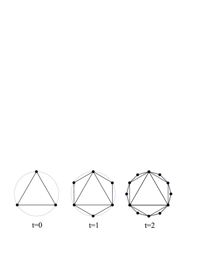
Figure 1: Illustration of the growing small-world network for $m=2$ and $q=1$, showing the first three steps of the iterative process.

When $q=1$ and $m=2$, the network is reduced to the deterministic ZRG model [42]. If $q<1$, the network is growing randomly. Especially, as $q$ approaches to zero (without reaching this value) the model coincides with the OHO model [41], where at each time step, only one interval is chosen and linked to its $m$ nearest neighbors, with every interval having the same probability of being selected (see [43] for interpretation). Varying $q$ in the interval (0,1) allows one to study the crossover between the OHO model [41] and the ZRG model [42]. It should be mentioned that as $q$ is a real number, below we will assume that all variables concerned with $q$ change continuously. Notice that similar presumption has been used in Refs. [1, 2, 3], which is valid in the limit of large $t$.

Now we compute the number of nodes and edges of $N(t)$. We denote the number of newly added nodes and edges at step $t$ by $L_{v}(t)$ and $L_{e}(t)$, respectively. Thus, initially ($t=0$), we have $L_{v}(0)=m+1$ nodes and $L_{e}(0)=m(m+1)/2$ edges in $N(0)$. Let $N_{c}(t)$ denote the total number of internode intervals along the ring at step $t$, then $N_{c}(0)=m+1$. By construction, we have $L_{v}(t)=N_{c}(t-1)q$ for arbitrary $t\geq 1$. Note that, when a new node is added to the network, an interval is destroyed and replaced by two new intervals, hence the number of total intervals increases by one. Thus, we have the following relation: $N_{c}(t)=N_{c}(t-1)+L_{v}(t)$. On the other hand, the addition of each new node leads to $m$ new edges, after simple calculations one can obtain that at $t_{i}$ ($t_{i}\geq 1$), $L_{v}(t_{i})=(m+1)(1+q)^{t_{i}-1}q$ and $L_{e}(t_{i})=m(m+1)(1+q)^{t_{i}-1}q$, respectively. Therefore, the number of nodes $N_{t}$ and the total of edges $E_{t}$ of $N(t)$ is

$$N_{t}=\sum_{t_{j}=0}^{t}L_{v}(t_{j})=(m+1)(1+q)^{t}$$ (1)

and

$$E_{t}=\sum_{t_{j}=0}^{t}L_{e}(t_{j})=m(m+1)\left[(1+q)^{t}-\frac{1}{2}\right]$$ (2)

respectively. The average node degree is then

$$<k>_{t}=\frac{2E_{t}}{N_{t}}=2m\left[1-\frac{1}{2(1+q)^{t}}\right]$$ (3)

For large $t$ and any $q\neq 0$, it is small and approximately equal to $2m$. Notice that many real-life networks are sparse in the sense that the number of edges in the network is much less than $N_{t}(N_{t}-1)/2$, the number of all possible edges [1, 2, 3].

3 Structural properties of the evolving small-world Network

Structural properties of the networks are of fundamental significance to understand the complex dynamics of real-life systems. Here we focus on four important characteristics: degree distribution, clustering coefficient, average path length and diameter.

3.1 Degree distribution

Degree is the simplest and most intensively studied characteristic of an individual node. The degree of a node $i$ is the number of edges in the whole network connected to $i$. The degree distribution $P(k)$ is defined as the probability that a randomly selected node has exactly $k$ edges. Let $k_{i}(t)$ denote the degree of node $i$ at step $t$. If node $i$ is added to the network at step $t_{i}$ then, by construction, $k_{i}(t_{i})=m$. In each of the subsequent time steps, there are $m$ intervals with $\frac{m}{2}$ at each side of $i$. Each of these intervals could be considered, with probability $q$, to create a new node connected to $i$. Then the degree $k_{i}(t)$ of node $i$ satisfies the relation

$$k_{i}(t)=k_{i}(t-1)+mq$$ (4)

considering the initial condition $k_{i}(t_{i})=m$, we obtain

$$k_{i}(t)=m+mq(t-t_{i})$$ (5)

The degree of each node can be obtained explicitly as in Eq. 5, and we see that this degree increases at each iteration. So it is convenient to obtain the cumulative distribution [3]

$$P_{cum}(k)=\sum_{k^{\prime}=k}^{\infty}P(k^{\prime})$$ (6)

which is the probability that the degree is greater than or equal to $k$. An important advantage of the cumulative distribution is that it can reduce the noise in the tail of probability distribution. Moreover, for some networks whose degree distributions have exponential tails: $P(\tilde{k})\sim e^{-\tilde{k}/\kappa}$, cumulative distribution also gives exponential expression with the same exponent:

$$P_{cum}(\tilde{k})=\sum_{k^{\prime}=\tilde{k}}^{\infty}P(k^{\prime})\sim\sum_{k^{\prime}=\tilde{k}}^{\infty}e^{-k^{\prime}/\kappa}\sim e^{-\tilde{k}/\kappa}$$ (7)

This makes exponential distributions particularly easy to spot experimentally, by plotting the corresponding cumulative distributions on semilogarithmic scales.

Using Eq. 5, we have $P_{cum}(k)=\sum_{k^{\prime}=k}^{\infty}P(k)=P\left(t^{\prime}\leq\tau=t-(\frac{k-m}{mq})\right)$. Hence

$$P_{cum}(k)=\sum_{t^{\prime}=0}^{\tau}\frac{L_{v}(t^{\prime})}{N_{t}}=\frac{m+1}{(m+1)(1+q)^{t}}+\sum_{t^{\prime}=1}^{\tau}\frac{(m+1)(1+q)^{t^{\prime}-1}q}{(m+1)(1+q)^{t}}$$

$$=(1+q)^{-\frac{k-m}{mq}}$$ (8)

The cumulative distribution decays exponentially with $k$. Thus the resulting network is an exponential network. Note that most small-world networks including the WS model belong to this class [7].

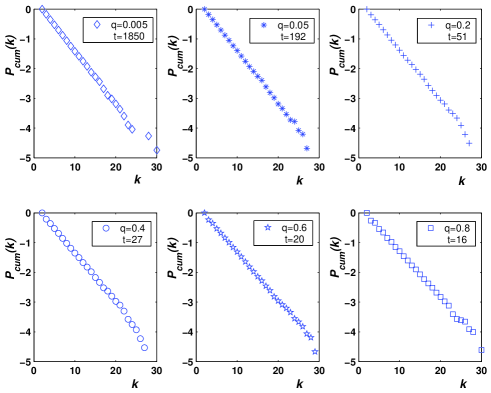
Figure 2: Semilogarithmic graph of the cumulative degree distribution for the evolving networks in the case of $m=2$ and for different values of $q$. All data points are obtained by averaging ten independent simulations.

In Fig. (2), we report the simulation results of the cumulative degree distribution for several values of $q$ and with $m=2$. Except in the deterministic case $q=1$, the degree spectrum of the networks is continuous. From Fig. (2), we can see that the cumulative degree distribution decays exponentially for large degree values, in agreement with the analytical results and supporting a relatively homogeneous topology similar to most small-world networks [5, 11, 22, 24, 25, 26, 27, 41]. Other values of $m$ should give qualitatively a similar behavior as for $m=2$.

3.2 Clustering coefficient

Most real-life networks show a cluster structure which can be quantified by the clustering coefficient [1, 2, 3, 4]. The clustering of a node gives the relation of connections of the neighborhood nodes closest to it. By definition, the clustering of a node $i$ with $k_{i}$ adjacent nodes is given by $C_{i}=2e_{i}/[k_{i}(k_{i}-1)]$, where $e_{i}$ is the number of existing edges between its neighbors. The clustering coefficient $C$ of a network is obtained by averaging $C_{i}$ over all the vertices in the network.

For the particular case $m=2$, using the connection rules, it is straightforward to calculate exactly the clustering coefficient of an arbitrary node and the average value for the network. When a node $i$ enters the network, $k_{i}$ and $e_{i}$ are $2$ and $1$, respectively. After that, if the degree $k_{i}$ increases by one, then its new neighbor must connect one of its existing neighbors, i.e. $e_{i}$ increases by one at the same time. Therefore, $e_{i}$ is equal to $k_{i}-1$ for all vertices at all time steps. So there exists a one-to-one correspondence between the degree of a node and its clustering. For a node $v$ with degree $k$, the exact expression for its clustering coefficient is $2/k$, which has been also been obtained in Ref. [32, 42, 44]. This expression for the local clustering shows the same inverse proportionality with the degree than the observed in a variety of real-life networks [34].

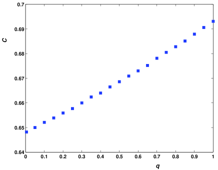
Figure 3: Average clustering coefficient $C$ vs $q$ when $m=2$. Each data point is an average over ten independent simulation runs.

In addition to the good scaling of the clustering coefficient for single node, the average clustering coefficient $C$ of the network is very high. Also, $C$ depends on $q$ and approaches to a constant asymptotic value as the network order is very large. In Fig. (3), we show $C$ as a function of $q$ in the case of $m=2$. From Fig. (3), one can see in the infinite order limit of the network, that $C$ approaches to a nonzero constant value. Simulations exhibit that $C$ equals to $0.6482$, $0.6560$, $0.6640$, $0.6729$ and $0.6828$ for $q=0.005$, $0.2$, $0.4$, $0.6$, and $0.8$, respectively. Fig. (3) reflects the dependence of $C$, the clustering coefficient of the network, on $q$. It is obvious that $C$ increases continuously with $q$. As $q$ increases from 0 to 1, $C$ grows from $\frac{3}{2}\ln 3-1$ [41] to $\ln 2$ [42], i.e. from $0.6479$ to $0.6931$. The reason for this dependence relation would need further study, but might be related to a biased choice of the edges chosen at each iteration, see Ref. [45]. Although we only focus on the case $m=2$, one expects that for other values of $m$, $C$ also will converge to a different nonzero value for every different value of $q$ (see Ref. [41] for a particular case).

3.3 Average path length

Certainly, the most important property for an small-world network is a logarithmic average path length (APL) (with the number of nodes). It has obvious implications for the dynamics of processes taking place on networks. Therefore, its study has attracted much attention. Here APL means the minimum number of edges connecting a pair of nodes, averaged over all pairs of nodes. Below, using an approach similar to that presented in [46], we will study the APL of our network for the particular case $m=2$.

We label each of the network nodes according to their creation times, $v=1,2,3,\ldots,N-1,N.$ We denote $L(N)$ as the APL of our network with order $N$. It follows that $L(N)=\frac{2\varepsilon(N)}{N(N-1)}$, where $\varepsilon(N)=\sum_{1\leq i<j\leq N}\ell_{i,j}$ is the total distance, where $\ell_{i,j}$ is the smallest distance between node $i$ and $j$.

For this special case $m=2$, any newly-created node is actually only attached to both ends of an edge. Thus the distances between existing node pairs will not be affected by the addition of new vertices. Then we have the following equation:

$$L(N+1)=L(N)+\sum_{i=1}^{N}\ell_{i,N+1}$$ (9)

Like in the analysis of [46, 47], Eq. (9) can be rewritten approximately as:

$$L(N+1)\approx L(N)+N+(N-2)L(N-1)$$ (10)

After some derivations, we can provide an upper bound for the variation of $\varepsilon(N)$ as

$${d\varepsilon(N)\over dN}=N+{2\varepsilon(N)\over N}$$ (11)

which leads to

$$\varepsilon(N)=N^{2}\ln N+\beta,$$ (12)

where $\beta$ is a constant. As $\varepsilon(N)\sim N^{2}\ln N$, we have $L(N)\sim\ln N$. Therefore, we have proved that in the special case of $m=2$ of our model, there is an slow growth of the APL with the network size $N$. In Fig. (4), we present the APL vs the network order $N$ in the case of $m=2$ and $q=0.5$. We see that the APL behaves logarithmically as a function of $N$. We expect that for other values of $q$, the APL will present a similar behavior. In fact, in the case of $q=1$, we can compute exactly the diameter of the network (i.e. the maximum distance between all pairs of nodes). A sharp analytical proof shows that the diameter also grows logarithmically with the number of nodes of the network [42]. It should be noted that in our model, considering values of $m$ greater than 2, then the APL will increase more slowly than in the case $m=2$ as in those cases the larger $m$ is, the denser the network becomes.

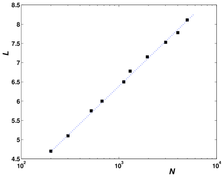
Figure 4: Semilogarithmic graph of the dependence of average path length on network order $N$ in the case of $m=2$ and $q=0.5$. All values plotted are averages over ten independent realizations. The values can be fitted well by a straight line.

Similar to Refs. [41, 42], the interpretation for the slow growth of APL is as follows. The older nodes that had once been geographically proximal along the ring are pushed apart as new nodes are positioned in the interval between them. From Fig. 1 we can see that when new nodes enter into the network, the original nodes are not near but, rather, have many newer nodes inserted between them. Thus, the network growth creates ”shortcuts” attached to old nodes, which join remote nodes along the ring one another as in the WS model [5].

3.4 Diameter for deterministic networks

As we have mentioned above the diameter of a network is the maximum of the distances between all pairs of nodes, characterizing the longest communication delay in the network. Small diameter is consistent with the concept of small-world. In the deterministic case $q=1$, we denote $N(t)$ as $N_{q=1}(t)$ and $Diam(N_{q=1}(t))$ as the diameter of $N_{q=1}(t)$ which can be computed exactly. But here we only give an upper bound on the diameter. The obtained bound scales logarithmically with the order of the networks. Now we present the main ideas of this analysis as follows.

Clearly, at step $t=0$, $Diam(N_{q=1}(0))$ equals to 1. At each step $t\geq 1$, we call newly-created nodes at this step active nodes. Since all active nodes are attached to those nodes existing in $N_{q=1}(t-1)$, so one can easily see that the maximum distance between arbitrary active node and those nodes in $N_{q=1}(t-1)$ is not more than $Diam(N_{q=1}(t-1))+1$ and that the maximum distance between any pair of active nodes is at most $Diam(N_{q=1}(t-1))+2$. Thus, at any step, the diameter of the network increases by 2 at most. Then we get $2(t+1)$ as an upper bound of $Diam(N(t)$. Note that the logarithm of $N_{q=1}(t)$ is $\ln((m+1)2^{t})=t\ln 2+\ln(m+1)$, which is approximately equal to $(t+1)\ln 2$ in the limit of large $t$. Thus the diameter grows at most logarithmically with the network order. Since our aim here is to show that the network diameter is small, so we only give a rough upper on diameter not more exact than that in [42].

4 Conclusion

To sum up, we give here a simple evolving model for small-world networks. During the network growth, new nodes do not have a complete knowledge of all the current network nodes, but are attached to those preexisting sites that are geographically close to them. We have obtained both analytically and numerically the solution for relevant parameters of the network and we have verified that our model exhibits the classical characteristics of small-world network: a high clustering and a short APL. In addition, the model under consideration is actually a tunable generalization which includes as particular extreme cases the models introduced in Refs. [41] and [42]. Moreover, the networks can model a variety of real-life networks whose topologies are influenced by such geographical constraints.

Acknowledgment

This research was supported by the Natural Science Foundation of China (Grant No. 70431001). Support for F.C. was provided by the Secretaria de Estado de Universidades e Investigación (Ministerio de Educación y Ciencia), Spain, and the European Regional Development Fund (ERDF) under project TIC2002-00155.

References

References

- [1] R. Albert and A.-L. Barabási, Rev. Mod. Phys. 74 (2002) 47.
- [2] S.N. Dorogovtsev and J.F.F. Mendes, Adv. Phys. 51 (2002) 1079.
- [3] M.E.J. Newman, SIAM Review 45 (2003) 167.
- [4] M.E.J. Newman, J. Stat. Phys. 101 (2000) 819.
- [5] D.J. Watts and S.H. Strogatz, Nature 393 (1998) 440.
- [6] M. Barthélémy and L.A.N. Amaral, Phys. Rev. Lett. 82 (1999) 3180.
- [7] A. Barrat, and M. Weigt, Eur. Phys. J. B 13 (2000) 547.
- [8] L.A.N. Amaral, A. Scala, M. Barthélémy and H.E. Stanley, PNAS, 97 (2000) 11149.
- [9] V. Latora and M. Marchiori, Phys. Rev. Lett. 87 (2001) 198701.
- [10] S.A. Pandit and R.E. Amritkar, Phys. Rev. E 60 (1999) R1119.
- [11] M.E.J. Newman and D.J. Watts, Phys. Lett. A 263 (1999) 341.
- [12] C.F. Moukarzel, Phys. Rev. E 60 (1999) 6263.
- [13] S.A. Pandit and R.E. Amritkar, Phys. Rev. E 63 (2001) 041104.
- [14] T. Nishikawa, A.E. Motter, Y.C. Lai and F.C. Hoppensteadt, Phys. Rev. E 66 (2002) 046139.
- [15] K. Medvedyeva, P. Holme, P. Minnhagen and B.J. Kim, Phys. Rev. E 67 (2003) 036118.
- [16] S.Y. Huang, X.W. Zou, Z.J. Tan, Z.G. Shao and Z.Z. Jin, Phys. Rev. E 68 (2003) 016107.
- [17] C.P. Herrero and M. Saboyá, Phys. Rev. E 68 (2003) 026106.
- [18] L.A. Braunstein, S.V. Buldyrev, R. Cohen, S. Havlin and H.E. Stanley, Phys. Rev. Lett. 91 (2003) 168701.
- [19] H. Guclu and G. Korniss Phys. Rev. E 69 (2004) 065104.
- [20] P. Blanchard and T. Krueger, Phys. Rev. E 71 (2005) 046139.
- [21] R. Monasson, Eur. Phys. J. B, 12 (1999) 555.
- [22] M.E.J. Newman and D.J. Watts, Phys. Rev. E 60 (1999) 7332.
- [23] M.E.J. Newman, C. Moore and D.J. Watts, Phys. Rev. Lett. 84 (2000) 3201.
- [24] R. Kasturirangan, Preprint Cond-mat/9904055.
- [25] S.N. Dorogovtsev and J.F.F. Mendes, Europhys. Lett. 50 (2000) 1.
- [26] J. Kleinberg, Nature 406 (2000) 845.
- [27] J. Kleinberg, Proceeding of the 32nd ACM Symposium on Theory of Computing (2000) 163.
- [28] F. Comellas, J. Ozón, and J.G. Peters, Inf. Process. Lett. 76 (2000) 83.
- [29] F. Comellas and M. Sampels, Physica A 309 (2002) 231.
- [30] A.-L. Barabási, E. Ravasz, and T. Vicsek, Physica A 299 (2001) 559.
- [31] K. Iguchi and H. Yamada, Phys. Rev. E 71 (2005) 036144.
- [32] S.N. Dorogovtsev, A.V. Goltsev, and J.F.F. Mendes, Phys. Rev. E 65 (2002) 066122.
- [33] S. Jung, S. Kim, and B. Kahng, Phys. Rev. E 65 (2002) 056101.
- [34] E. Ravasz and A.-L. Barabási, Phys. Rev. E 67 (2003) 026112.
- [35] J.D. Noh, Phys. Rev. E 67 (2003) 045103.
- [36] F. Comellas, G. Fertin, and A. Raspaud, Phys. Rev. E 69 (2004) 037104.
- [37] T. Zhou, B.H. Wang, P.M. Hui and K.P. Chan, Preprint Cond-mat/0405258.
- [38] J.S. Andrade Jr., H.J. Herrmann, R.F.S. Andrade and L.R. da Silva, Phys. Rev. Lett. 94 (2005) 018702.
- [39] J.P.K. Doye and C.P. Massen, Phys. Rev. E 71 (2005) 016128.
- [40] Z.Z. Zhang, F. Comellas, G. Fertin and L.L. Rong, Preprint Cond-mat/0503316.
- [41] J. Ozik, B.-R. Hunt, and E. Ott, Phys. Rev. E 69 (2004) 026108.
- [42] Z.Z. Zhang, L.L Rong and C.H. Guo, Preprint Cond-mat/0502335 (Physica A, in press).
- [43] S.N. Dorogovtsev, Phys. Rev. E 67 (2003) 045102.
- [44] S.N. Dorogovtsev, J.F.F. Mendes and A.N. Samukhin, Phys. Rev. E 63 (2001) 062101.
- [45] F. Comellas, H. D. Rozenfeld, D. ben-Avraham, arXiv: cond-mat/0508317 (Phys. Rev. E, in press).
- [46] T. Zhou, G. Yan and B.H. Wang, Phys. Rev. E 71 (2005) 046141.
- [47] Z.Z. Zhang, L.L. Rong and F. Comellas, Preprint Cond-mat/0502591 (Physica A in press).