Spin-correlation functions in ultracold paired atomic-fermion systems:
sum rules, self-consistent approximations, and mean fields

Abstract

The spin response functions measured in multi-component fermion gases by means of rf transitions between hyperfine states are strongly constrained by the symmetry of the interatomic interactions. Such constraints are reflected in the spin f-sum rule that the response functions must obey. In particular, only if the effective interactions are not fully invariant in SU(2) spin space, are the response functions sensitive to mean field and pairing effects. We demonstrate, via a self-consistent calculation of the spin-spin correlation function within the framework of Hartree-Fock-BCS theory, how one can derive a correlation function explicitly obeying the f-sum rule. By contrast, simple one-loop approximations to the spin response functions do not satisfy the sum rule, except in special cases. As we show, the emergence of a second peak at higher frequency in the rf spectrum, as observed in a recent experiment in trapped ${}^{6}\text{Li}$, can be understood as the contribution from the paired fermions, with a shift of the peak from the normal particle response proportional to the square of the BCS pairing gap.

I Introduction

Exploring pairing and superfluidity in ultracold trapped multicomponent-fermion systems poses considerable experimental and theoretical challenges jila_bcs ; mit_bcs ; duke_capacity ; jila_noise ; georg . Recently, Chin et al. chin_rf have found evidence, by rf excitation, of a pairing gap in a two-component trapped ⁶Li gas over a range of coupling strengths. The experiment, concentrating on the lowest lying hyperfine states, $|\sigma\rangle=|1\rangle$, $|2\rangle$ and $|3\rangle$, with $m_{F}$ = 1/2, -1/2, and -3/2 respectively, measures the long wavelength spin-spin correlation function, and is analogous to NMR experiments in superfluid ³He nmr1 ; nmr2 . While at high temperatures the rf field absorption spectrum shows a single peak from unpaired atoms, at sufficiently low temperature a second higher frequency peak emerges, attributed to the contribution from BCS paired atoms. Theoretical calculations at the “one-loop” level of the spin response torma ; levin ; pieri support this interpretation.

In this paper we carry out a fully self-consistent calculation of the spin-spin correlation function relevant to the rf experiment, at the Hartree-Fock-BCS level, in order to understand the dependence of the response on mean field shifts and the pairing gap. The calculation requires going beyond the one-loop level, and summing bubbles to all orders, and is valid in the weakly interacting BCS regime, away from the BEC-BCS crossover – the unitarity limit. An important constraint on the mean field shifts was brought out by Leggett leggett via a sum-rule argument: For a system with an interaction that is SU(2)-invariant in spin space, the spins in the long-wavelength limit simply precess as a whole at the Larmor frequency, without mean field effects; then the spin-spin correlation function is dominated by a single pole at the Larmor frequency. While the effective interactions between the three lowest hyperfine states of ⁶Li are not SU(2)-invariant the f-sum rule obeyed by the spin-spin correlation function still, as we shall show, implies strong constraints on the spin response, which are taken into account via a self-consistent calculation.

In order to bring out the physics of a self-consistent approach to the spin response, we consider a spatially uniform system, and work within the framework of simple BCS theory on the “BCS side” of the Feshbach resonance where the interactions between hyperfine states are attractive. We assume an effective Hamiltonian in terms of the three lowest hyperfine states explicitly involved in the experiments chin_rf ; mit_rf (we take $\hbar=1$ throughout):

$$H = \int d\mathbf{r}\big{\{}\sum_{\sigma=1}^{3}\left(\frac{1}{2m}\nabla\psi^{\dagger}_{\sigma}(\mathbf{r})\cdot\nabla\psi_{\sigma}(\mathbf{r})+\epsilon^{\sigma}_{z}\psi^{\dagger}_{\sigma}(\mathbf{r})\psi_{\sigma}(\mathbf{r})\right)$$

$$+\frac{1}{2}\sum_{\sigma,\sigma^{\prime}=1}^{3}\bar{g}_{\sigma\sigma^{\prime}}\psi^{\dagger}_{\sigma}(\mathbf{r})\psi^{\dagger}_{\sigma^{\prime}}(\mathbf{r})\psi_{\sigma^{\prime}}(\mathbf{r})\psi_{\sigma}(\mathbf{r})\big{\}},$$

where $\psi_{\sigma}$ is the annihilation operator for state $|\sigma\rangle$, $\bar{g}_{\sigma\sigma^{\prime}}$ is the bare coupling constant between states $\sigma$ and $\sigma^{\prime}$, which we assume to be constant up to a cutoff $\Lambda$ in momentum space. Consistent with the underlying symmetry we assume $\Lambda$ to be the same for all channels, and take $\Lambda\to\infty$ at the end of calculating physical observables. The renormalized coupling constants $g_{\sigma\sigma^{\prime}}$ are related to those of the bare theory by

$$g^{-1}_{\sigma\sigma^{\prime}}=\bar{g}^{-1}_{\sigma\sigma^{\prime}}+m\Lambda/2\pi^{2},$$ (2)

where, in terms of the s-wave scattering length $a_{\sigma\sigma^{\prime}}$, $g_{\sigma\sigma^{\prime}}=4\pi a_{\sigma\sigma^{\prime}}/m$. In evaluating frequency shifts in normal states, we implicitly resum particle-particle ladders involving the bare couplings and generate the renormalized couplings. However, to treat pairing correlations requires working directly in terms of the bare $\bar{g}_{\sigma\sigma^{\prime}}$ legg .

It is useful to regard the three states $|\sigma\rangle$ as belonging to a pseudospin (denoted by $Y$) multiplet with the eigenvalues $m_{\sigma}$ of $Y_{z}$ equal to 1,0,-1 for $\sigma$ = 1,2,3. In terms of $m_{\sigma}$ the Zeeman splitting of the three levels is

$$\epsilon_{Z}^{\sigma}=\epsilon_{Z}^{2}-(\epsilon_{Z}^{3}-\epsilon_{z}^{1})m_{\sigma}/2+(\epsilon_{Z}^{3}+\epsilon_{Z}^{1}-2\epsilon_{Z}^{2})m_{\sigma}^{2}/2.$$ (3)

The final term in ⁶Li is of order 4% of the middle term on the BCS side. The interatomic interactions in the full Hamiltonian for the six $F=1/2$ and $F=3/2$ hyperfine states are invariant under the SU(2) group of spin rotations generated by the total spin angular momentum $\mathbf{F}$. The effective Hamiltonian can be derived from the full Hamiltonian by integrating out the upper three levels. However, because the effective interactions between the lower three levels depend on the non-SU(2) invariant coupling of the upper states to the magnetic field, the interactions in the effective Hamiltonian (LABEL:ch) are no longer SU(2) invariant length ; shizhong .

In the Chin et al. experiment equal numbers of atoms were loaded into states $|1\rangle$ and $|2\rangle$ leaving state $|3\rangle$ initially empty; transitions of atoms from $|2\rangle$ to $|3\rangle$ were subsequently induced by an rf field. Finally the residue atoms in $|2\rangle$ were imaged, thus determining the number of atoms transferred to $|3\rangle$. The experiment (for an rf field applied along the $x$ direction) basically measures the frequency dependence of the imaginary part of the correlation function $(-i)\int d^{3}r\langle T\left(\psi^{\dagger}_{2}(\mathbf{r},t)\psi_{3}(\mathbf{r},t)\psi^{\dagger}_{3}(0,0)\psi_{2}(0,0)\right)\rangle$ (although in principle atoms can make transitions from $|2\rangle$ to $|4\rangle$; such a transition, at higher frequency, is beyond the range studied in the experiment, and is not of interest presently). Here $T$ denotes time ordering. This correlation function can be written in terms of long-wavelength pseudospin-pseudospin correlation function, the Fourier transform of

$$\chi_{xx}(t)=-i\langle T\left(Y_{x}(t)Y_{x}(0)\right)\rangle;$$ (4)

here $Y_{x}=\int d^{3}ry_{x}(\mathbf{r})$ is the $x$ component of the total pseudospin of the system,

$$y_{x}(\mathbf{r}) = \frac{1}{\sqrt{2}}\big{(}\psi^{\dagger}_{1}(\mathbf{r})\psi_{2}(\mathbf{r})+\psi^{\dagger}_{2}(\mathbf{r})\psi_{1}(\mathbf{r})$$ (5)

$$+\psi^{\dagger}_{2}(\mathbf{r})\psi_{3}(\mathbf{r})+\psi^{\dagger}_{3}(\mathbf{r})\psi_{2}(\mathbf{r})\big{)}$$

is the local pseudospin density along the x-axis. Since the experiment is done in a many-body state with $N_{1}=N_{2}$, the contribution from transitions between $|1\rangle$ and $|2\rangle$ is zero SY . The Fourier transform of $\chi_{xx}(t)$ has the spectral representation,

$$\chi_{xx}(\Omega)=\int^{\infty}_{-\infty}\frac{d\omega}{\pi}\frac{{\chi}^{\prime\prime}_{xx}(\omega)}{\Omega-\omega},$$ (6)

where $\chi^{\prime\prime}_{xx}(\omega)={\rm Im}\chi_{xx}(\omega-i0^{+})$.

In the next section we discuss the f-sum rule in general, review Leggett’s argument, and illustrate how the sum rule works in simple cases. Then in Section III we carry out a systematic calculation, within Hartree-Fock-BCS theory, of the spin-spin correlation functions, generating them from the single particle Green’s functions. In addition to fulfilling the f-sum rule, our results are consistent with the emergence of the second absorption peak observed in the rf spectrum at low temperature from pairing of fermions.

II Sum rules

The f-sum rule obeyed by the pseudospin-pseudospin correlation function arises from the identity,

$$\int^{+\infty}_{-\infty}\frac{d\omega}{\pi}\omega{\chi}^{\prime\prime}_{xx}(\omega)=\langle[[Y_{x},H],Y_{x}]\rangle.$$ (7)

The need for self-consistency is driven by the fact that the commutator on the right side eventually depends on the single particle Green’s function, whereas the left side involves the correlation function. The static pseudospin susceptibility, $-\chi_{xx}(0)$, is related to ${\chi}^{\prime\prime}_{xx}(\omega)$ by

$$\chi_{xx}(0)=-\int^{\infty}_{-\infty}\frac{d\omega}{\pi}\frac{{\chi}^{\prime\prime}_{xx}(\omega)}{\omega}.$$ (8)

Leggett’s argument that an SU(2) invariant system gives an rf signal only at the Larmor frequency is the following: Let us assume that the $\bar{g}_{\sigma\sigma^{\prime}}$ are all equal, so that the interaction in Eq. (LABEL:ch) is SU(2) invariant in pseudospin space; in addition, let us assume, for the sake of the argument, that the Zeeman energy is $-\gamma m_{\sigma}B_{z}$ ($\gamma$ is the gyromagnetic ratio of the pseudospin). Then the right side of Eq. (7) becomes $\gamma B_{z}\langle Y_{z}\rangle$, while the static susceptibility, $-\chi_{xx}(0)$, equals $\langle Y_{z}\rangle/\gamma B_{z}$. In this case, the spin equations of motion imply that the response is given by a single frequency (as essentially found experimentally nmr1 ; nmr2 ). Thus for $\omega>0$, we take $\chi^{\prime\prime}_{xx}(\omega)$ to be proportional to $\delta(\omega-\omega_{0})$. Combining Eqs. (7) and (8), we find $\omega_{0}=\gamma B_{z}$, the Larmor frequency. The sum rule implies that neither mean field shifts nor pairing effects can enter the long wavelength rf spectrum of an SU(2) invariant system.

It is instructive to see how the sum rule (7) functions in relatively simple cases. We write the space and time dependent spin density correlation function as

$$D_{xx}(10)\equiv-i\langle T\left(y_{x}(1)y_{x}(0)\right)\rangle$$

$$=\frac{1}{2}[D_{12}(1)+D_{21}(1)+D_{23}(1)+D_{31}(1)],$$ (9)

where

$$D_{\beta\alpha}(1)\equiv -i\langle T\left(\psi^{\dagger}_{\alpha}(1)\psi_{\beta}(1)\psi^{\dagger}_{\beta}(0)\psi_{\alpha}(0)\right)\rangle,$$ (10)

and $\alpha,\beta=1,2,3$. Here $\psi(1)$, with $1$ standing for $\{\mathbf{r}_{1},t_{1}\}$, is in the Heisenberg representation, with Hamiltonian $H^{\prime}=H-\sum_{\sigma}\mu_{\sigma}N_{\sigma}$. Equation (9) implies that $\chi^{\prime\prime}_{xx}$ is a sum of $\chi^{\prime\prime}_{\beta\alpha}$, where

$$\chi_{\beta\alpha}(\Omega)\equiv\frac{V}{2}D_{\beta\alpha}(\mathbf{q}=0,\Omega+\mu_{\alpha}-\mu_{\beta}),$$ (11)

and $V$ is the system volume.

As a first example we consider free particles (denoted by superscript $0$). For $\alpha\neq\beta$,

$$D^{0}_{\beta\alpha}(1)= -iG^{0}_{\alpha}(-1)G_{\beta}^{0}(1).$$ (12)

where $G^{0}_{\alpha}(1)$, the free single particle Green’s function, has Fourier transform, $G^{0}_{\alpha}(\mathbf{k},z)=1/(z-e^{\alpha}_{k})$, with $z$ the Matsubara frequency and $e^{\alpha}_{k}=k^{2}/2m+\epsilon_{Z}^{\alpha}-\mu_{\alpha}$. Then,

$$\chi^{0}_{\beta\alpha}(\Omega)=\frac{1}{2}\frac{N_{\alpha}-N_{\beta}}{\Omega+\epsilon_{Z}^{\alpha}-\epsilon_{Z}^{\beta}},$$ (13)

from which we see that ${\chi^{0}}^{\prime\prime}_{\beta\alpha}(\omega)$ has a delta function peak at $\epsilon_{Z}^{\beta}-\epsilon_{Z}^{\alpha}$, as expected for free particles. This result is manifestly consistent with Eq. (7).

Next we take interactions into account within the Hartree-Fock approximation (denoted by $H$) for the single particle Green’s function, with an implicit resummation of ladders to change bare into renormalized coupling constants. It is tempting to factorize $D$ as in the free particle case as torma ; levin ; pieri ; btrz ; OG ,

$$D^{H0}_{\beta\alpha}(1)=-iG^{H}_{\alpha}(-1)G_{\beta}^{H}(1),$$ (14)

where $G^{H}_{\alpha}(\mathbf{k},z)=1/(z-\zeta^{\alpha}_{k})$, with

$$\zeta^{\alpha}_{k}=\frac{k^{2}}{2m}+\epsilon_{Z}^{\alpha}+\sum_{\beta(\neq\alpha)}g_{\alpha\beta}n_{\beta}-\mu_{\alpha}$$ (15)

and $n_{\beta}$ the density of particles in hyperfine level $\beta$. Then

$$D^{H0}_{\beta\alpha}(\mathbf{q}=0,\Omega)=\frac{n_{\alpha}-n_{\beta}}{\Omega+\zeta_{0}^{\alpha}-\zeta_{0}^{\beta}},$$ (16)

and

$$\chi_{\beta\alpha}(\Omega)=\hskip 180.0pt$$

$$\frac{1}{2}\frac{N_{\alpha}-N_{\beta}}{\Omega+\epsilon_{Z}^{\alpha}+\sum_{\sigma(\neq\alpha)}g_{\alpha\sigma}n_{\sigma}-\epsilon_{Z}^{\beta}-\sum_{\sigma^{\prime}(\neq\beta)}g_{\beta\sigma^{\prime}}n_{\sigma^{\prime}}}.$$

Consequently

$$\chi^{\prime\prime}_{\beta\alpha}(\omega) = -\frac{\pi}{2}(N_{\beta}-N_{\alpha})\delta(\omega-\Delta E_{\beta\alpha}),$$ (18)

where

$$\Delta E_{\beta\alpha}=\epsilon_{Z}^{\beta}+\sum_{\sigma^{\prime}(\neq\beta)}g_{\beta\sigma^{\prime}}n_{\sigma^{\prime}}-\epsilon_{Z}^{\alpha}-\sum_{\sigma(\neq\alpha)}g_{\alpha\sigma}n_{\sigma}$$ (19)

is the energy difference of the single particle levels $|\alpha\rangle$ and $|\beta\rangle$. The response function $\chi^{\prime\prime}_{\beta\alpha}(\omega)$ is non-zero only at $\omega=\Delta E_{\beta\alpha}$.

On the other hand, $\chi^{\prime\prime}_{\beta\alpha}(\omega)$ obeys the sum rule

$$\int^{+\infty}_{-\infty}\frac{d\omega}{\pi}\omega{\chi}^{\prime\prime}_{\beta\alpha}(\omega)$$

$$=\frac{V}{2}\int d^{3}\mathbf{r}\langle[[\psi^{\dagger}_{\alpha}(\mathbf{r})\psi_{\beta}(\mathbf{r}),H],\psi^{\dagger}_{\beta}(0)\psi_{\alpha}(0)]\rangle$$ (20)

$$=\frac{1}{2}(N_{\alpha}-N_{\beta})\Big{(}\Delta E_{\beta\alpha}-g_{\alpha\beta}(n_{\beta}-n_{\alpha})\Big{)}.$$ (21)

where the final line holds for the Hartree-Fock approximation. The sum rule (21) is violated in this case unless $g_{\alpha\beta}=0$.

The self-consistent approximation for the correlation function (detailed in the following section) that maintains the sum rule and corresponds to the Hartree approximation for the single particle Green’s function includes a sum over bubbles in terms of the renormalized $g$’s:

$$D^{H}_{\beta\alpha}(q,\Omega)=\frac{D^{H0}_{\beta\alpha}(q,\Omega)}{1+g_{\beta\alpha}D^{H0}_{\beta\alpha}(q,\Omega)}.$$ (22)

Then with (22),

$$\chi_{\beta\alpha}{{}^{\prime\prime}}(\omega)=\frac{\pi}{2}(N_{\alpha}-N_{\beta})\delta\Big{(}\omega+(\epsilon_{Z}^{\alpha}-\epsilon_{Z}^{\beta}$$

$$+\sum_{\sigma(\neq\alpha)}g_{\alpha\sigma}n_{\sigma}-\sum_{\rho(\neq\beta)}g_{\beta\rho}n_{\rho}+g_{\alpha\beta}(n_{\beta}-n_{\alpha}))\Big{)}.$$ (23)

Note that $\chi_{32}{{}^{\prime\prime}}(\omega)$ peaks at $\omega_{H}=\epsilon_{Z}^{3}-\epsilon_{Z}^{2}+(g_{13}-g_{12})n_{1}$, indicating that the mean field shift is $(g_{13}-g_{12})n_{1}$.

This result agrees with the rf experiment done in a two level ${}^{6}{\rm Li}$ system away from the resonance region mit_two . This experiment finds that no matter whether the atoms in states $|1\rangle$ and $|2\rangle$ are coherent or incoherent, the rf signal of the transition between $|1\rangle$ and $|2\rangle$ never shows a mean field shift. As explained in mit_two , in a coherent sample, the internal degrees of freedom of all the fermions are the same, and thus there is no interaction between them. In the incoherent case, the above calculation gives $\chi_{12}{{}^{\prime\prime}}(\omega)=(\pi/2)(N_{2}-N_{1})\delta(\omega+\epsilon_{Z}^{2}-\epsilon_{Z}^{1})$, always peaking at the difference of the Zeeman energy, and therefore without a mean field contribution. hydrogen

In an rf experiment using all three lowest hyperfine states, the mean field shifts appear in $\chi^{H}_{32}{{}^{\prime\prime}}$ as $(g_{13}-g_{12})n_{1}$. Since $g_{\sigma\sigma^{\prime}}=4\pi a_{\sigma\sigma^{\prime}}\hbar^{2}/m$, our result $(g_{13}-g_{12})n_{1}$ agrees with Eq. (1) of Ref. mit_rf . However, from $B$ =660 to 900 G (essentially the region between the magnetic fields at which $a_{13}$ and $a_{12}$ diverge) no obvious deviation of the rf signal from the difference of the Zeeman energies is observed in the unpaired state mit_rf ; chin_private . The frequency shifts estimated from the result (23) taken literally in this region do not agree with experiment; one should not, however, trust the Hartree-Fock mean field approximation around the unitarity limit. The disappearance of the mean field shifts in the unitary regime has been attributed to the s-wave scattering process between any two different species of atoms becoming unitary-limited chin_rf ; torma ; however, the situation is complicated by the fact that the two two-particle channels do not become unitarity limited simultaneously.

III Self-consistent approximations

References baym and baymkad laid out a general method to generate correlation functions self-consistently from the single particle Green’s functions. To generate the correlation function $\chi_{xx}(t)$, defined in Eq. (4), we couple the pseudospin to an auxiliary field $F(\mathbf{r},t)$, analogous to the rf field used in the experiments, via the probe Hamiltonian :

$$H_{\rm probe}(t)= -\int d\mathbf{r}F(\mathbf{r},t)y_{x}(\mathbf{r}).$$ (24)

The single particle Green’s function is governed by the Hamiltonian $H^{\prime}$, together with the probe Hamiltonian. The procedure is to start with an approximation to the single particle Green’s function, and then generate the four-point correlation function by functional differentiation with respect to the probe field. Using this technique we explicitly calculate the pseudospin-pseudospin correlation functions consistent with the Hartree-Fock-BCS approximation for the single particle Green’s function, in a three-component interacting fermion system, relevant to the rf experiment on the BCS side ($g_{\sigma\sigma^{\prime}}<0$).

To calculate the right side of Eq. (7) directly, we decompose the Hamiltonian as $H=H_{\rm invar}+H_{\rm var}$, where $H_{\rm invar}$ is invariant under SU(2) and the remainder

$$H_{\rm var}=\epsilon_{Z}^{2}+(\epsilon_{Z}^{3}+\epsilon_{Z}^{1}-2\epsilon_{Z}^{2})Y_{z}^{2}/2-(\epsilon_{Z}^{3}-\epsilon_{Z}^{1})Y_{z}/2$$

$$+(\bar{g}_{13}-\bar{g}_{12})\int\psi_{3}^{\dagger}\psi_{1}^{\dagger}\psi_{1}\psi_{3}+(\bar{g}_{23}-\bar{g}_{12})\int\psi_{3}^{\dagger}\psi_{2}^{\dagger}\psi_{2}\psi_{3},$$

is not invariant. We evaluate the right side of Eq. (7), $\langle[[Y_{x},H_{\rm var}],Y_{x}]\rangle$, term by term in the case that the states have particle number $N_{1}=N_{2}=N$ and $N_{3}=0$, The Zeeman energy in $H_{\rm var}$ gives $(\epsilon_{Z}^{3}-\epsilon_{Z}^{2})N$, and the second term gives $(\bar{g}_{12}-\bar{g}_{13})\int\langle\psi_{2}^{\dagger}\psi_{1}^{\dagger}\psi_{1}\psi_{2}\rangle$.

We factorize the correlation function within the Hartree-Fock-BCS theory for the contact pseudopotential in (LABEL:ch), implicitly resumming ladders to renormalize the coupling constant in the direct and exchange terms dilute , to write,

$$(\bar{g}_{12}-\bar{g}_{13}) \int \langle\psi_{2}^{\dagger}\psi_{1}^{\dagger}\psi_{1}\psi_{2}\rangle$$ (26)

$$= (g_{12}-g_{13})\int\langle\psi_{2}^{\dagger}\psi_{2}\rangle\langle\psi_{1}^{\dagger}\psi_{1}\rangle$$

$$+(\bar{g}_{12}-\bar{g}_{13})\int\langle\psi_{2}^{\dagger}\psi_{1}^{\dagger}\rangle\langle\psi_{1}\psi_{2}\rangle.$$

Using Eq. (2), we find a contribution from the second term, $V(g_{12}-g_{13})(n_{2}n_{1}+|\Delta|^{2}/g_{12}g_{13})$, where $\Delta\equiv\langle\psi_{1}\psi_{2}\rangle/\bar{g}_{12}$, is the BCS pairing gap between $|1\rangle$ and $|2\rangle$, assumed to be real and positive. The last term gives $(\bar{g}_{12}-\bar{g}_{23})\int\int\int\langle{\psi_{2}^{\dagger}}^{\prime}\psi_{3}^{\prime}\psi_{3}^{\dagger}\psi_{2}^{\dagger}\psi_{2}\psi_{3}{\psi_{3}^{\dagger}}^{\prime\prime}\psi_{2}^{\prime\prime}\rangle=0$; altogether,

$$\int^{\infty}_{-\infty}\frac{d\omega}{\pi}\omega\chi^{\prime\prime}_{xx}(\omega)\hskip 144.0pt$$

$$=(\epsilon_{Z}^{3}-\epsilon_{Z}^{2})N-V(g_{12}-g_{13})\left(n_{1}n_{2}+\Delta^{2}/g_{12}g_{13}\right).$$ (27)

The absence of $g_{23}$ arises from $N_{3}$ being zero. Were all $g_{\sigma\sigma^{\prime}}$ equal, the right side of Eq. (27) would reduce to $(\epsilon^{3}_{Z}-\epsilon^{2}_{Z})N$, as expected. When the interaction is not SU(2) invariant both mean field shifts and the pairing gap contribute to the sum rule, allowing the possibility of detecting pairing via the rf absorption spectrum.

We turn now to calculating the full Hartree-Fock-BCS pseudospin-pseudospin correlation function. For convenience we define the spinor operator

$$\Psi=\left(\psi_{1},\psi_{2},\psi_{3},\psi^{\dagger}_{1},\psi^{\dagger}_{2},\psi^{\dagger}_{3}\right),$$ (28)

and calculate the single particle Green’s function

$$G_{ab}(1,1^{\prime})\equiv(-i)\langle T\Psi_{a}(1)\Psi_{b}^{\dagger}(1^{\prime})\rangle,$$ (29)

where $1$ denotes $r_{1},t_{1}$, etc., and the subscripts $a$ and $b$ run from 1 to 6 (in the order from left to right in Eq. (28); the subscripts 4, 5, and 6 should not be confused with the label for the upper three hyperfine states), and $\Psi_{a}(1)$ is in the Heisenberg representation with Hamiltonian $H^{\prime\prime}=H^{\prime}+H_{\rm probe}(t)$. For $F(\mathbf{r},t)=0$ and with BCS pairing between $|1\rangle$ and $|2\rangle$,

$$G=\pmatrix{G_{11}&0&0&0&G_{15}&0\cr 0&G_{22}&0&G_{24}&0&0\cr 0&0&G_{33}&0&0&0\cr 0&G_{42}&0&G_{44}&0&0\cr G_{51}&0&0&0&G_{55}&0\cr 0&0&0&0&0&G_{66}}.$$ (30)

To obtain a closed equation for $G_{ab}(1,1^{\prime})$, we factorize the four-point correlation functions in the equation of motion for $G$ as before, treating the Hartree-Fock (normal propagator) and BCS (abnormal propagator) parts differently. In the dynamical equation for $G_{11}(1,2)$, the term $\bar{g}_{12}\langle\psi^{\dagger}_{2}(1)\psi_{2}(1)\psi_{1}(1)\psi^{\dagger}_{1}(2)\rangle$ is approximated as $g_{12}\langle\psi^{\dagger}_{2}(1)\psi_{2}(1)\rangle\langle\psi_{1}(1)\psi^{\dagger}_{1}(2)\rangle$ for the normal part, but $\bar{g}_{12}\langle\psi_{2}(1)\psi_{1}(1)\rangle\langle\psi^{\dagger}_{2}(1)\psi^{\dagger}_{1}(2)\rangle$ for the abnormal part legg . Since $n_{1}=n_{2}$, $\epsilon_{Z}^{1}+g_{12}n_{2}+g_{13}n_{3}-\mu_{2}=\epsilon_{Z}^{2}+g_{12}n_{1}+g_{23}n_{3}-\mu_{2}\equiv-\mu_{0}$, where $\mu_{0}$ is the free particle Fermi energy; $\mu_{0}$ enters into the single particle Green’s function as usual via the dispersion relation $E_{k}\equiv\left[(k^{2}/2m-\mu_{0})^{2}+\Delta^{2}\right]^{1/2}$ for the paired states.

The equation of the single particle Green’s function in matrix form is

$$\int d\bar{1}\{{G_{0}}^{-1}(1\bar{1})-F(1)\tau\delta(1-\bar{1})$$

$$-\Sigma(1\bar{1})\}G(\bar{1}1^{\prime}) =\delta(1-1^{\prime}),$$ (31)

where the inverse of the free single-particle Green’s function is

$${G^{0}}^{-1}_{ab}(11^{\prime})=\left(i\frac{\partial}{\partial t_{1}}+\frac{\nabla^{2}_{1}}{2m}\pm\mu_{a}\right)\delta(1-1^{\prime})\delta_{ab},$$ (32)

with the upper sign for $a$=1,2,3, and the lower for $a$=4,5,6. The matrix $\tau$ is

$$\tau=\frac{1}{\sqrt{2}}\left(\begin{array}[]{rrrrrr}0&1&0&0&0&0\\ 1&0&1&0&0&0\\ 0&1&0&0&0&0\\ 0&0&0&0&-1&0\\ 0&0&0&-1&0&-1\\ 0&0&0&0&-1&0\end{array}\right).$$ (39)

The self energy takes the form

$$-i\Sigma(11^{\prime})=\hskip 440.0pt$$

$$\small\pmatrix{-g_{12}G_{22}-g_{13}G_{33}&g_{12}G_{12}&g_{13}G_{13}&0&-\bar{g}_{12}G_{15}&-\bar{g}_{13}G_{16}\cr g_{12}G_{21}&-g_{12}G_{11}-g_{23}G_{33}&g_{23}G_{23}&-\bar{g}_{12}G_{24}&0&-\bar{g}_{23}G_{26}\cr g_{13}G_{31}&g_{23}G_{32}&-g_{13}G_{11}-g_{23}G_{22}&-\bar{g}_{13}G_{34}&-\bar{g}_{23}G_{35}&0\cr 0&\bar{g}_{12}G_{51}&\bar{g}_{13}G_{61}&g_{12}G_{22}+g_{13}G_{33}&-g_{12}G_{21}&-g_{13}G_{31}\cr\bar{g}_{12}G_{42}&0&\bar{g}_{23}G_{62}&-g_{12}G_{12}&g_{12}G_{11}+g_{23}G_{33}&-g_{23}G_{32}\cr\bar{g}_{13}G_{43}&\bar{g}_{23}G_{53}&0&-g_{13}G_{13}&-g_{23}G_{23}&g_{13}G_{11}+g_{23}G_{22}},$$

where here $G_{ab}$ denotes $G_{ab}(11^{+})\delta(1-1^{\prime})$ with $1^{+}=\{\mathbf{r}_{1},t_{1}+0^{+}\}$.

We generate the correlation functions as

$$D_{ab}(12)=-i\sqrt{2}\left(\frac{\delta G_{ab}(11^{+})}{\delta F(2)}\right)_{F=0};$$ (42)

(where the factor $\sqrt{2}$ cancels that from the coupling of $F(\mathbf{r},t)$ to the atoms via $y_{x}$) so that from Eq. (31),

$$D(q,\Omega) = \frac{\sqrt{2}}{\beta V}\sum_{k,z}G(k,z)\left(\tau\right.$$ (43)

$$+\frac{\delta\Sigma}{\delta B_{\rm rf}}(q,\Omega)\left.\right)G(k-q,z-\Omega).$$

Using Eq. (30) in (43), we derive

$$D_{23}=\frac{D^{0}_{23}}{1+g_{23}D^{0}_{23}},$$ (44)

$$D_{12}=\frac{D^{0}_{12}}{1+g_{12}D^{0}_{12}},$$ (45)

where

$$D^{0}_{23}=\Pi_{2233}+\bar{g}_{13}\frac{\Pi_{2433}\Pi_{6651}}{1-\bar{g}_{13}\Pi_{6611}},$$ (46)

and

$$D^{0}_{12}=\Pi_{1122}-\Pi_{1542};$$ (47)

the bubble $\Pi_{abcd}(q,\Omega)$ is given by

$$\Pi_{abcd}(q,\Omega)=\frac{1}{\beta V}\sum_{k,z}G_{ab}(k,z)G_{cd}(k-q,z-\Omega),$$ (48)

and the summation on $k$ is up to $\Lambda$. When $\Delta\to 0$, Eqs. (44) and (45) reduce to (22), since $\Pi_{2433}$ and $\Pi_{6511}$ are both proportional to $\Delta$. Furthermore, when the interaction is SU(2) invariant, $\chi^{\prime\prime}_{32}(\omega)$ is proportional to $\delta(\omega-(\epsilon_{z}^{3}-\epsilon_{z}^{2}))$. If only $\bar{g}_{12}$ is non-zero, the response function $D_{23}$ reduces to the single loop, $\Pi_{2233}$ (as calculated in Ref. pieri ), and in fact satisfies the f-sum rule (7).

To see that the result (44) for the correlation function obeys the sum rule (27), we expand Eq. (44) as a power series in $1/\Omega$ in the limit $\Omega\to\infty$ and compare the coefficients of $1/\Omega^{2}$ of both sides. In addition, with $n_{1}=n_{2}$, we find $\int(d\omega/2\pi)\omega\chi^{\prime\prime}_{12}(\omega)=0$.

Figure (1) shows the paired fermion contribution to $\chi_{32}^{\prime\prime}(\omega)$, calculated from Eqs. (44) and (11), as a function of $\omega$, with $g_{\sigma,\sigma^{\prime}}=4\pi\hbar^{2}a_{\sigma,\sigma^{\prime}}/m$. This graph corresponds to the ⁶Li experiment done in a spatially uniform system. The origin is the response frequency of unpaired atoms, which is $\omega_{32}^{H}=\epsilon_{z}^{3}-\epsilon_{z}^{2}+(g_{13}-g_{12})n_{1}$. We have not included the normal particle response in our calculation and do not show this part of the response in the figure. The parameters used are $k_{F}a_{12}=-\pi/4$ and $a_{13}=a_{23}=0.1a_{12}$, for which, $T_{c}=0.084\mu_{0}$. As the pairing gap, $\Delta$, grows with decreasing temperature, the most probable frequency, $\omega_{\rm pair}$, in the response shifts to higher value. Within the framework of BCS theory, we can interpret the peak at higher frequency observed in the rf experiment as the contribution from the paired atoms.

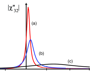
Figure 1: (Color online). The pseudospin response function, $|\chi_{32}^{\prime\prime}|$, vs. $\omega$ for $k_{F}a_{12}=-\pi/4$ and $a_{13}=a_{23}=0.1a_{12}$ for three temperatures. The curves correspond to a) $T$ = 0.0831, $\Delta$ = 0.0084, b) $T$ = 0.0830, $\Delta$ = 0.012, and c) $T$ = 0.0820, $\Delta$ = 0.030, all in units of the free particle Fermi energy in hyperfine states $|1\rangle$ and $|2\rangle$.

We now ask how the most probably frequency $\omega_{\rm pair}$ is related to the pairing gap $\Delta$. To do this we use the sum rule (27) on $\chi^{\prime\prime}_{xx}(\omega)$, written in terms of $\chi^{\prime\prime}_{32}(\omega)$. Since $\chi^{\prime\prime}_{xx}(\omega)=\chi^{\prime\prime}_{32}(\omega)+\chi^{\prime\prime}_{23}(\omega)$ and $\chi^{\prime\prime}_{32}(-\omega)=-\chi^{\prime\prime}_{23}(\omega)$, we have

$$\int^{\infty}_{-\infty}\frac{d\omega}{\pi}\omega\chi^{\prime\prime}_{xx}(\omega)=2\int^{\infty}_{-\infty}\frac{d\omega}{\pi}\omega\chi^{\prime\prime}_{32}(\omega).$$ (49)

Formally expanding Eq. (44) as a power series in $1/\Omega$ and comparing the coefficients of $1/\Omega$ on both sides, we find

$$\int^{\infty}_{-\infty}\frac{d\omega}{\pi}\chi^{\prime\prime}_{32}(\omega)=\langle Y_{z}\rangle/2.$$ (50)

Then assuming that the rf peak due to pairing is single and narrow (as found experimentally), we approximate $\chi^{\prime\prime}_{32}(\omega)$ as $\pi\langle Y_{z}\rangle\delta(\omega-\omega_{\rm pair})/2$. Using Eqs. (27), (49) and (50), we finally find

$$\omega_{\rm pair}-\omega_{H}=(g_{13}-g_{12})\frac{\Delta^{2}}{n_{0}g_{12}g_{13}},$$ (51)

where $n_{0}=n_{1}=n_{2}$. Thus BCS pairing shifts the spectrum away from the normal particle peak by an amount proportional to $\Delta^{2}$.

Equation (51) enables one to deduce the pairing gap $\Delta$ from the experimental data in the physical case, $g_{13}\neq 0$. However this result breaks down for the paired states when $g_{13}=0$, a consequence of the dependence of the sum rule in Eq. (27) on the cutoff $\Lambda$ of the bare model (LABEL:ch). To see this point, we note that the factor $(g_{13}-g_{12})/g_{12}g_{13}$ that multiplies $\Delta^{2}$ in Eq. (27) arises from the combination of the bare coupling constants $1/\bar{g}_{12}-\bar{g}_{13}/\bar{g}_{12}^{2}$; using Eq. (2) we can write this combination in terms of the renormalized coupling constants and the cutoff as

$$g_{12}^{-1}-\frac{m\Lambda}{2\pi^{2}}-\frac{(g_{12}^{-1}-m\Lambda/2\pi^{2})^{2}}{g_{13}^{-1}-m\Lambda/2\pi^{2}}.$$ (52)

Expanding in $1/\Lambda$ in the limit $\Lambda\to\infty$, we see that the terms linear in $\Lambda$ cancel, leaving the cutoff-independent result, $g_{13}^{-1}-g_{12}^{-1}$, as in Eqs. (27) and (51). However, if only $\bar{g}_{12}$ is nonzero in this model then we find the cutoff-dependent result,

$$\omega_{\rm pair}-\omega_{H} = \frac{\Delta^{2}}{n_{0}\bar{g}_{12}}=\frac{\Delta^{2}}{n_{0}}(\frac{1}{g_{12}}-\frac{m\Lambda}{2\pi^{2}}).$$ (53)

Fitting the measured shift in Ref. chin_rf , Fig. 2, to Eq. (51), using the values of $a_{12}$ and $a_{13}$ as functions of magnetic field given in Ref. mit_rf , and assuming that $g_{\sigma\sigma^{\prime}}=4\pi\hbar^{2}a_{\sigma\sigma^{\prime}}/m$, we find that for Fermi energy, $E_{F}=3.6\mu$K, $\Delta/E_{F}$ = 0.23 at 904G ($k_{F}a_{13}=-1.58$, $k_{F}a_{12}=-3.92$), and 0.27 at 875G (or in terms of the Fermi momentum, $k_{F}a_{13}=-1.69$, $k_{F}a_{12}=-6.31$). Similarly for $E_{F}=1.2\mu$K, $\Delta/E_{F}$ = 0.14 at 904G ($k_{F}a_{13}=-0.91$, $k_{F}a_{12}=-2.26$), and 0.19 at 875G ($k_{F}a_{13}=-0.98$, $k_{F}a_{12}=-3.64$). These values are in qualitative agreement with theoretical expectations gaps , although we expect corrections to the result (51) in the regime where the $k_{F}a$ are not small, and in finite trap geometry.

IV Conclusion

As we have seen, the experimental rf result on the BCS side can be understood by means of a self-consistent calculation of the pseudospin response within the framework of BCS theory in the manifold of the lowest three hyperfine states. The second peak observed at low temperature arises from pairing between fermions, with the displacement of the peak from the normal particle peak proportional to the square of the pairing gap $\Delta$. The shift of the peak vanishes if the interactions within the lowest three states is SU(2) invariant. Although the results given here are for the particular case of the lowest hyperfine states in ⁶Li, the present calculation can be readily extended to other multiple component fermion systems, as well as extended to include effects of the finite trap in realistic experiments.

We thank Tony Leggett, Shizhong Zhang, and Cheng Chin for valuable discussions. This work was supported in part by NSF Grants PHY03-55014 and PHY05-00914.

References

• (1) C.A. Regal, M. Greiner and D.S. Jin, Phys. Rev. Lett. 92, 040403 (2004).
• (2) M.W. Zwierlein, C.A. Stan, C.H. Schunck, S.M.F. Raupach, A.J. Kerman and W. Ketterle, Phys. Rev. Lett. 92, 120403 (2004).
• (3) J. Kinast, A. Turlapov, J.E. Thomas, Q. Chen, J. Stajic, and K. Levin, Science 307 1296 (2005).
• (4) M. Greiner, C.A. Regal, J.T. Stewart, and D.S. Jin, Phys. Rev. Lett. 94, 110401 (2005).
• (5) G.M. Bruun and G. Baym, Phys. Rev. Lett. 93, 150403 (2004).
• (6) C. Chin, M. Bartenstein, A. Altmeyer, S. Riedl, S. Jochim, J. Hecker Denschlag and R. Grimm, Science 305, 1128 (2004).
• (7) D.D. Osheroff, R.C. Richardson, and D.M. Lee, Phys. Rev. Lett. 28, 885 (1972).
• (8) D.D. Osheroff, W. J. Gully, R.C. Richardson, and D.M. Lee, Phys. Rev. Lett. 29, 920 (1972).
• (9) J. Kinnunen, M. Rodríguez and P. Törmä, Science 305, 1131 (2004).
• (10) Y. He, Q. Chen, and K. Levin, cond-mat/0504394.
• (11) P. Pieri, A. Perali, and G.C. Strinati, to be published.
• (12) A.J. Leggett, Phys. Rev. Lett. 29, 1227 (1972).
• (13) S. Gupta, Z. Hadzibabic, M.W. Zwierlein, C.A. Stan, K. Dieckmann, C.H. Schunck, G.M. van Kempen, B.J. Verhaar and W. Ketterle, Science 300, 1723 (2003).
• (14) A. J. Leggett, J. Phys. (Paris) C7, 19 (1980).
• (15) M. Bartenstein, A. Altmeyer, S. Riedl, R. Geursen, S. Jochim, C. Chin, J.H. Denschlag and R. Grimm, Phys. Rev. Lett. 94 103201 (2005); C. Chin and P.S. Julienne, Phys. Rev. A 71, 012713 (2005).
• (16) S. Zhang, to be published.
• (17) The coupling of the rf field to the atoms at the magnetic fields of interest in the Chin et al. experiment is primarily through the electron spin. The contribution to the electron spin-spin correlation function from transitions between the lower three hyperfine states is
$\displaystyle\langle T\left(S_{x}(t)S_{x}(0)\right)\rangle/V\hskip 120.0pt$
$\displaystyle\hskip 20.0pt=|\langle 2|S_{x}|3\rangle|^{2}\int d^{3}r\left(\langle T\psi^{\dagger}_{2}(\mathbf{r},t)\psi_{3}(\mathbf{r},t)\psi^{\dagger}_{3}(0,0)\psi_{2}(0,0)\rangle\right.$
$\displaystyle\left.+c.c.\right)$
$\displaystyle+|\langle 1|S_{x}|2\rangle|^{2}\int d^{3}r\left(\langle T\psi^{\dagger}_{1}(\mathbf{r},t)\psi_{2}(\mathbf{r},t)\psi^{\dagger}_{2}(0,0)\psi_{1}(0,0)\rangle\right.$
$\displaystyle\left.+c.c.\right),$
where $V$ is the volume. Since the latter term vanishes in the many-body state with $N_{1}=N_{2}$, $N_{3}=0$, we have simply,
$\displaystyle\langle T\left(S_{x}(t)S_{x}(0)\right)\rangle=\frac{|\langle 2|S_{x}|3\rangle|^{2}}{|\langle 2|Y_{x}|3\rangle|^{2}}\langle T\left(Y_{x}(t)Y_{x}(0)\right)\rangle.$
• (18) G.M. Bruun, P. Torma, M. Rodriguez and P. Zoller, Phys. Rev. A 64, 033609 (2001).
• (19) Y. Ohashi and A. Griffin, Phys. Rev. A 72, 013601 (2005).
• (20) M.W. Zwierlein, Z. Hadzibabic, S. Gupta and W. Ketterle, Phys. Rev. Lett. 91, 250404 (2003).
• (21) A counterpart calculation for binary bosonic systems with $n_{1}\neq 0$ and $n_{2}=0$ gives the rf signal shift as $8\pi(a_{11}-a_{12})n_{1}/m$, compared with the mean field shift $4\pi(2a_{11}-a_{12})n_{1}/m$ expected by the direct factorization calculation pethick , resolving the mysterious factor $2$ observed in front of $a_{12}$ in spin-polarized hydrogengreytak .
• (22) C.J. Pethick and H.T.C. Stoof, Phys. Rev. A, 64, 013618 (2001).
• (23) T.C. Killian, D.G. Fried, L. Willmann, D. Landhuis, S.C. Moss, T.J. Greytak, and D. Kleppner, Phys. Rev. Lett. 81, 3807 (1998).
• (24) C. Chin, private communication.
• (25) G. Baym, Phys. Rev. 127, 1391 (1962).
• (26) G. Baym and L.P. Kadanoff, Phys. Rev. 124, 287 (1961).
• (27) An exact self-consistent calculation that starts from the bare interaction and sums particle-particle ladders to generate the renormalized interaction includes terms in the correlation functions involving internal particle loops, as in the last term in Fig. 4c of Ref. baymkad . However, these terms are of relative order $k_{F}a$, the Fermi momentum times the relevant scattering length, and in the weak interaction limit can be neglected compared with the terms we calculate here.
• (28) M. Holland, S.J.J.M.F. Kokkelmans, M.L. Chiofalo, and R. Walser, Phys. Rev. Lett. 87, 120406 (2001); Y. Ohashi and A. Griffin, Phys. Rev. 89, 130402 (2002); J. Carlson, S.-Y. Chang, V.R. Pandharipande, and K.E. Schmidt, Phys. Rev. Lett. 91, 050401 (2003), G. Ortiz and J. Dukelsky, Phys. Rev. A 72, 043611 (2005).