Properties of the strongly paired fermionic condensates

Abstract

We study a gas of fermions undergoing a wide resonance $s$-wave BCS-BEC crossover, in the BEC regime at zero temperature. We calculate the chemical potential and the speed of sound of this Bose-Einstein-condensed gas, as well as the condensate depletion, in the low density approximation. We discuss how higher order terms in the low density expansion can be constructed. We demonstrate that the standard BCS-BEC gap equation is invalid in the BEC regime and is inconsistent with the results obtained here. The low density approximation we employ breaks down in the intermediate BCS-BEC crossover region. Hence our theory is unable to predict how the chemical potential and the speed of sound evolve once the interactions are tuned towards the BCS regime. As a part of our theory, we derive the well known result for the bosonic scattering length diagrammatically and check that there are no bound states of two bosons.

I Introduction

In their seminal papers A. Leggett Leggett (1980) and P. Nozières and R. Schmitt-Rink Nozières and Schmitt-Rink (1985) studied a system of spin-1/2 fermions with attractive short-ranged interactions in the singlet channel at low temperature. If the interactions are weak, the fermions form a Bardeen-Cooper-Schrieffer (BCS) superconductor. If the interactions are made progressively stronger, at some critical interaction strength a bound state of two fermions becomes possible. These bound states are then bosons, which undergo Bose-Einstein condensation (BEC). Studies by these and many other authors demonstrated that as the interaction strength is increasing, the BCS superfluid smoothly evolves into the BEC superfluid, without undergoing any phase transition in between.

Quite remarkably, Leggett, and Nozières and Schmitt-Rink afterwards, found that the BCS gap equation, the mean-field equation which describes the properties of the BCS superconductor, evolves under the strengthening of the potential into the Schrödinger equation of a bound pair of fermions. This happens despite the fact that the gap equation is derived on the assumption of weak interactions between the fermions and should in principle break down as the interaction strength is increased. Interestingly, this observation was first made as far back as in 1966 by V. N. Popov, Popov (1966), but his contribution, at least within the context of the BCS-BEC crossover, was not noticed until later. Similarly, the BCS-BEC crossover was first studied in 1969 by D. M. Eagles Eagles (1969) while the two channel model Timmermans et al. (1999) was first studied by Yu. B. Rumer Rumer (1959).

The fact that the gap equation describes the BCS superconductor well, combined with the fact that the gap equation is also well suited to describe the bound pairs of fermions on the opposite side of the crossover, and taking into account that there is no phase transition in between, allowed Nozières and Schmitt-Rink to conclude that it may be used to interpolate between these two regimes, when the potential is neither too weak nor too strong and the fermions form an intermediate crossover BCS-BEC superfluid.

Interest in this subject was recently revived when the BCS-BEC superfluid was obtained experimentally in the cold atomic systems where the interactions can be tuned with the help of Feshbach resonances Timmermans et al. (1999); Holland et al. (2001); Timmermans et al. (2001); Strecker et al. (2003); Regal et al. (2004); Zwierlein et al. (2004). Thus for the first time theoretical predictions regarding the BCS-BEC crossover can be tested experimentally.

Given the lack of justification for the gap equation in the BEC regime beyond predicting the binding energy of a pair of fermions, the question remained whether it can be used to predict other properties of the BEC condensate, such as the condensate depletion, excitation spectrum and so on.

In this paper, we show that the gap equation is actually not valid on the BEC side of the crossover. Although correctly predicting the binding energy of the fermionic bound pairs, it fails to describe the interactions of these dimers properly. As a result, if taken literally, it incorrectly predicts the physical properties of the BEC superfluid.

Indeed, it is generally believed in the literature Leggett (1980); Nozières and Schmitt-Rink (1985) that the transition between the BCS and the BEC phases occurs without a phase transition making these phases qualitatively the same phase. Thus on a qualitative level, it is possible to use the gap equation to obtain order of magnitude estimates of the parameters of the BEC phase. However, if one is interested in quantitative calculations, one needs to go beyond the gap equation. Barring the exact solution of the problem, which most likely is not possible here, the next best thing is to identify a small parameter and do the calculations as an expansion in powers of that parameter. The gap equation, when written on the BEC side of the crossover, implicitly assumes that the small parameter is the interaction strength between the bosons. This assumption is invalid; it has been known for some time now that the Born approximation fails to describe the interactions between the bosons properly Petrov et al. (2005).

In this paper, we identify as a small parameter the so-called gas parameter of the Bose gas, and do all calculations as an expansion in powers of that parameter.

The gap equation should be replaced by another equation on the BEC side of the crossover. That equation, described below, cannot be derived exactly, but can only be obtained as an expansion in powers of the gas parameter. In the lowest order approximation, it allows us to compute the chemical potential $\mu_{b}$, the speed of sound $u$ in the superfluid, and the condensate depletion to be, at zero temperature,

$$\mu_{b}=\frac{4\pi n_{b}}{m_{b}}a_{b},\,\,\,u^{2}=\frac{4\pi n_{b}}{m_{b}^{2}}a_{b},$$

$$n_{0,b}=n_{b}\left[1-\frac{8}{3}\sqrt{\frac{n_{b}\,a_{b}^{3}}{\pi}}\right].$$ (1)

Here

$$a_{b}\approx 0.60\,a$$ (2)

is the scattering length of the bosonic dimers, whose approximate relationship to the scattering length of a pair of fermions $a$ has first been derived by Petrov, Salomon, and Shlyapnikov Petrov et al. (2005). The coefficient $0.60$ is approximate in the sense of being determined only numerically, although the procedure to find it is in principle exact. $n_{b}$ is the density of bosons, which in the lowest order approximation in density can be replaced by $n/2$, where $n$ is the density of the fermions. $n_{0,b}$ is the condensate density. $m_{b}=2m$ is the mass of the bosons, where $m$ is the fermion mass. $\mu_{b}$ is the chemical potential of the bosons, which can be related to the chemical potential $\mu$ of the fermions by demanding that $\mu_{b}-2\mu$ coincides with the binding energy released when the boson is formed. Throughout this paper we adopt units in which $\hbar=1$.

Our results Eq. (I) coincide with the behavior of the dilute interacting Bose gas Abrikosov et al. (1977). We would like to emphasize that they are not exact, but are obtained as the lowest order approximation in powers of the gas parameter $an^{\frac{1}{3}}$. It is possible to use the techniques described in this paper and calculate the next order corrections to Eq. (I). They will no longer necessarily coincide with the next order corrections in the standard dilute Bose gas. We will not calculate them here, however, and limit our discussion with merely indicating how these higher order corrections can be obtained.

As the BEC condensate is tuned towards the crossover BCS-BEC regime, $a$ increases reaching infinity at the unitary point which lies somewhere in the intermediate BCS-BEC region. Thus the approximation used in this paper breaks down as the intermediate regime is approached. Our technique is unable to tell us anything about the crossover regime, and we will not attempt to study it in this paper.

All calculations in this paper are done at zero temperature. We think that our techniques can also be adopted to finite temperatures, including studies of the critical superfluid transition temperature, either in the large $N$ approximation or using some other technique. See also Ref. Andersen (2004) for more references on this subject. We will not attempt to do this in this paper.

It is important to note that the interaction potential between fermions is characterized not only by the scattering length $a$, but also by the effective range $r_{0}$. Unlike $a$ which changes as the interaction potential is tuned through the crossover, $r_{0}$ remains roughly the same. If $\left|r_{0}\right|\gg n^{-\frac{1}{3}}$, then the fermions are said to be in the narrow resonance regime. In that regime, the gap equation is a good approximation to the actual physics of the BCS-BEC crossover everywhere Gurarie and Radzihovsky (2005). However, the wide resonance crossover where $\left|r_{0}\right|\ll n^{-\frac{1}{3}}$, $\left|r_{0}\right|\ll\left|a\right|$ is more relevant for the current experiments, and it is the wide resonance crossover which received most attention in the literature. Everything we described above this paragraph pertains to the wide resonance regime. In order to be certain that we work in the wide resonance regime, we employ the one channel model which guarantees that $r_{0}$ is vanishingly small.

An important part of the theory presented in this paper is the diagrammatic derivation of Eq. (2). It has come to our attention that while our work was in progress, this was derived diagrammatically, independently of us, by I. V. Brodsky, M. Y. Kagan, A. V. Klaptsov, R. Combescot, and X. Leyronas, in Ref. Brodsky et al. (2005). The techniques these authors employed to arrive at Eq. (2) coincide with the ones discussed here.

Finally, we note that a problem similar to the one studied in this paper was examined by L. V. Keldysh and A. N. Kozlov in the context of excitons in Ref. Keldysh and Kozlov (1968). Those authors, however, concentrated on the case of Coulomb interactions of interest for the physics of excitons, while we are interested in short ranged interactions, which have quite a different physics. In particular, the universal results Eq. (I) do not hold for their system. Additionally, they, as well as Ref. Popov (1966), used an operator version of perturbation theory which is hard to generalize beyond the lowest order. In contrast, our theory is based on a functional integral and is easily generalizable to arbitrary order. It is still remarkable that these authors understood the breakdown of the gap equation in the BEC regime long before this became an important issue in the BCS-BEC crossover literature.

The rest of the paper is organized as follows. In section II we introduce the formalism and discuss how the calculations of interest to us can be performed. In section III we set up a perturbative expansion in powers of the gas parameter. In the next section IV we perform the actual calculations and derive Eq. (I). Section V discusses an alternative derivation of the results of section IV and the origin of the breakdown of the BCS-BEC gap equation. Finally, in section VI, which is followed by conclusions, we compute the scattering amplitude between bosons and the bosonic scattering length Eq. (2), a necessary step in the calculations performed in this paper. Some of the technical details of the calculations are discussed in the appendices.

II Formulation of the problem

Consider a gas of spin-1/2 fermions, interacting with some short ranged interaction in the $s$-wave channel. The most straightforward way to study this gas is by means of a functional integral

$$Z=\int{\cal D}\bar{\psi}_{\uparrow}{\cal D}\psi_{\uparrow}{\cal D}\bar{\psi}_{\downarrow}{\cal D}\psi_{\downarrow}~{}e^{iS_{f}},$$ (3)

where $S_{f}=S_{0}+S_{\rm int}$ is the action consisting of the free part

$$S_{0}=\sum_{\sigma=\uparrow,\downarrow}\int d^{3}x~{}dt~{}\bar{\psi}_{\sigma}\left(i\frac{\partial}{\partial t}+\frac{1}{2m}\frac{\partial^{2}}{\partial{\bf x}^{2}}+\mu\right)\psi_{\sigma}$$ (4)

and the interaction part

$$S_{\rm int}=\lambda\int d^{3}x~{}dt~{}\bar{\psi}_{\uparrow}\bar{\psi}_{\downarrow}\psi_{\downarrow}\psi_{\uparrow}.$$ (5)

This term describes interactions which happen at one point in space. We need to remember that by itself such an interaction is unphysical and has to be supplemented by a momentum cutoff $\Lambda$. $\lambda>0$ to reflect that we choose an attractive interaction potential.

As is standard in the treatment of superconductivity, we introduce the Hubbard-Stratonovich field $\Delta$, which allows us to rewrite Eq. (3) in the equivalent way

$$Z=\int{\cal D}\bar{\psi}_{\uparrow}{\cal D}\psi_{\uparrow}{\cal D}\bar{\psi}_{\downarrow}{\cal D}\psi_{\downarrow}{\cal D}\Delta{\cal D}\bar{\Delta}~{}e^{iS},$$ (6)

where the action $S$ is now given by $S=S_{0}+S_{\rm HS}$, and

$$S_{\rm HS}=-\int d^{3}x~{}dt~{}\left[\frac{1}{\lambda}\bar{\Delta}\Delta+\left(\Delta\bar{\psi}_{\uparrow}\bar{\psi}_{\downarrow}+\bar{\Delta}\psi_{\downarrow}\psi_{\uparrow}\right)\right].$$ (7)

The total action $S$ is now quadratic in fermions, so the fermions can be integrated out. This results in the following partition function

$$Z=\int{\cal D}\Delta{\cal D}\bar{\Delta}~{}e^{iS_{\Delta}},$$ (8)

where the effective action $S_{\Delta}$ is given by

$$S_{\Delta} = -i~{}\hbox{tr}\,\log\left(\matrix{\omega^{+}-\frac{{\bf p}^{2}}{2m}+\mu&-\Delta\cr-\bar{\Delta}&\omega^{+}+\frac{{\bf p}^{2}}{2m}-\mu}\right)$$ (10)

$$-\frac{1}{\lambda}\int dtd^{3}x~{}\bar{\Delta}\Delta,$$

where $\omega^{+}=\omega+i0\,{\rm sign}~{}\omega$. The action $S_{\Delta}$ and the functional integral Eq. (8) represent the starting point in our theory, although sometimes it is also advantageous to keep the fermions explicitly, as in Eq. (6) and Eq. (7).

In the modern literature on Feshbach resonances, the system described in Eqs.(3), (4), and (5) is often referred to as the one channel model. The interactions between fermions in this model are such that their effective range $r_{0}$ is vanishingly small (in the limit of a large momentum cutoff $\Lambda$). And indeed, the results described in this paper are applicable to the limit $|r_{0}|\ll n^{-{\frac{1}{3}}}$, $\left|r_{0}\right|\ll\left|a\right|$ only, thus the one channel model is a natural starting point for our study. Alternatively, one could also study the two channel model Timmermans et al. (1999). The two channel model involves an additional parameter which allows control of the value of $r_{0}$ independently of $a$. However, if we chose to work with the two channel model, to ensure the smallness of $r_{0}$ we would need to study the limit of infinitely strong coupling within that model. In that limit, the distinction between the two channel and one channel models disappear. This is explained in more detail in Appendix A. Because of this equivalence, we will not study the two channel model any further in this paper.

The standard approach at this stage is to find the extremum of the action $S_{\Delta}$ with respect to the field $\Delta$. Assuming that the extremum of the action is when the field $\Delta$ takes some constant value $\Delta_{0}$, we find the BCS-BEC gap equation

$$\frac{1}{\lambda}=\frac{1}{2}\int\frac{d^{3}p}{(2\pi)^{3}}\frac{1}{\sqrt{\left(\frac{p^{2}}{2m}-\mu\right)^{2}+\Delta_{0}^{2}}}.$$ (11)

The integral in the gap equation is up to momenta of the order of the cutoff $\Lambda$. It is advantageous to trade the interaction strength $\lambda$ for the fermionic scattering length $a$ using the relation

$$a=\left(-\frac{4\pi}{m\lambda}+\frac{2\Lambda}{\pi}\right)^{-1}.$$ (12)

This relation is fairly standard. For completeness, we include its derivation in Appendix B. Then the BCS-BEC gap equation acquires the form

$$-\frac{m}{4\pi a}=\frac{1}{2}\int\frac{d^{3}p}{(2\pi)^{3}}\left[\frac{1}{\sqrt{\left(\frac{p^{2}}{2m}-\mu\right)^{2}+\Delta_{0}^{2}}}-\frac{2m}{p^{2}}\right].$$ (13)

The integral over momentum $p$ is now convergent and can be extended to infinity.

If $a$ is negative and $|a|n^{\frac{1}{3}}\ll 1$ (this corresponds to the weak attraction), then we say that the gas of fermions is in the BCS state. In this regime, the gap equation has been investigated in detail in the literature devoted to superconductors. It was shown that the fluctuations of $\Delta$ about its mean field value $\Delta_{0}$, which solves Eq. (13), are indeed small, and the physics of the superconductors can be captured by solving Eq. (13).

As the interaction strength is increased, $a$ becomes more and more negative, reaching negative infinity at the interaction strength which corresponds to the threshold of bound state creation. For even stronger potentials, $a$ becomes positive, first large and then it gets smaller. In this regime there is no justification for using Eq. (13).

Yet Ref. Nozières and Schmitt-Rink (1985) argued that in the “deep BEC” regime where $an^{\frac{1}{3}}\ll 1$, Eq. (13) can be reinterpreted as the Schrödinger equation of a pair of fermions, with chemical potential playing the role of half of the energy. So the gap equation then correctly predicts the formation of bosonic dimers. Indeed, solving the gap equation in this regime by anticipating that $\mu\ll-\Delta_{0}$, we neglect $\Delta_{0}$ and find within this approximation

$$\mu=-\frac{1}{2ma^{2}}.$$ (14)

$1/ma^{2}$ is the binding energy of two fermions, as expected.

Nevertheless there is no reason to expect that the gap equation holds beyond Eq. (14). For example, one could expect that attempting to use it to compute the deviation of $\mu$ from Eq. (14) due to nonzero $\Delta_{0}$ in Eq. (13) would lead to an incorrect relation between the boson chemical potential $\mu_{b}=2\mu+1/(ma^{2})$ and $\Delta_{0}$. On the other hand knowing the proper relation between $\mu_{b}$ and $\Delta_{0}$ would allow us to compute the physical properties of the BEC condensate, such as the speed of sound. So there is a need to develop a reliable technique which allows computation of these quantities.

In this paper we investigate the properties of the system in the low density “deep BEC” regime, that is, in the regime where $a$ is positive and small, so that $an^{\frac{1}{3}}\ll 1$. To this end, we will calculate the normal and anomalous propagators of the bosonic $\Delta$ field using a diagrammatic expansion. In doing so, we will keep only the diagrams lowest in the density of the system. However, we will not assume that the interactions are weak, or in other words, that the interactions can be treated in the Born approximation.

The fact that the Born approximation is not applicable to the bosonic dimers has been known for quite a while. Indeed, the dimer’s scattering length in the Born approximation is $a_{b}=2a$ Sá de Melo et al. (1993), while the correct scattering length is given by Eq. (2). Although first derived in Ref. Petrov et al. (2005) by solving the four-body Schrödinger equation, it can also be derived by summing all the diagrams contributing to the scattering exactly. In this paper we perform this summation and derive Eq. (2) diagrammatically in section VI. This allows us to recognize $a_{b}$ when the diagrams contributing to it appear within the diagrams for the normal and anomalous bosonic propagators in our theory.

Once the bosonic propagators are calculated, we will impose the condition that they have a pole at zero frequency and momentum, representing the sound mode of the condensate. This will give us a relation between the chemical potential $\mu$, the scattering length $a$, and the expectation value $\Delta_{0}$ of the field $\Delta$, which will replace the gap equation Eq. (13). In the dilute Bose gas literature, this is usually referred to as the Hugenholtz-Pines relation Hugenholtz and Pines (1959). This equation replaces the gap equation in our theory.

If instead of this proper procedure we had used the gap equation, we would have arrived at Eq. (I) with $a_{b}=2a$, which is the Born approximation to the dimer scattering length. Thus the gap equation fails because it cannot treat the interaction between dimers beyond Born approximation.

In order to be able to determine the unknown quantities $\mu$ and $\Delta_{0}$, one also needs another equation. Its role is usually played by the particle number equation, which states that the total particle density is equal to $n$,

$$n=\frac{1}{V}\int d^{3}x~{}\left[\left\langle\,\bar{\psi}_{\uparrow}\psi_{\uparrow}\,\right\rangle+\left\langle\,\bar{\psi}_{\downarrow}\psi_{\downarrow}\,\right\rangle\right],$$ (15)

where $V$ is the volume of the system. In its most naive incarnation, we calculate the particle density by assuming that the field $\Delta$ does not fluctuate and is equal to its mean value $\Delta_{0}$. Then we find

$$n=\int\frac{d^{3}p}{(2\pi)^{3}}\left[1-\frac{\frac{p^{2}}{2m}-\mu}{\sqrt{\left(\frac{p^{2}}{2m}-\mu\right)^{2}+\Delta_{0}^{2}}}\right].$$ (16)

We are going to show that this equation is indeed correct in the lowest order approximation in density. However, if one wants to go beyond the lowest order approximation, Eq. (16) acquires nontrivial corrections.

III Diagrammatic Expansion

To set up a diagrammatic expansion, we first write down free propagators which follow from Eq. (7) or Eq. (10), taking into account that we work in the BEC regime where $\mu<0$. The propagator of the fermions is given by

$$G_{0}(p,\omega)=\frac{1}{\omega-\frac{p^{2}}{2m}+\mu+i0}.$$ (17)

Note that since $\mu<0$, the propagator is retarded.

The propagator of bosons is, naively, equal to $-\lambda$. However, we also need to include in it the self energy correction due to fermionic loops. In other words, we need to expand the effective action $S_{\Delta}$ up to quadratic order in $\Delta$ and the corresponding term in the expansion corrects the propagator. This expansion is performed in Appendix B. We find, again taking into account that $\mu<0$,

$$D_{0}(p,\omega)=\frac{4\pi}{m}\frac{1}{a^{-1}-\sqrt{m}\sqrt{-\omega+\frac{p^{2}}{4m}-2\mu-i0}}.$$ (18)

The bosonic propagator is also retarded, as any propagator of free bosons must be at zero temperature Abrikosov et al. (1977).

The fact that all the free propagators are retarded crucially simplifies the diagrammatic expansion. Note that in the BCS regime where $\mu>0$ this simplification would not have taken place. Similar effect happens in the more standard dilute Bose gas Abrikosov et al. (1977).

The diagrammatic technique must also involve the lines beginning or ending in the condensate. These are assigned the value $\Delta_{0}$. Although $\Delta_{0}^{2}$ does not coincide with the density of particles in the condensate, it is proportional to it. In turn, the condensate density is always lower than the total density $n$. Thus the expansion in powers of the density $n$ can be replaced by the expansion in powers of $\Delta_{0}$. Since each line beginning or ending in the condensate is assigned the value $\Delta_{0}$, the expansion in the density can also be understood as the expansion in numbers of lines beginning or ending in the condensate.

Now we would like to construct self energy corrections to the propagators $G_{0}$ and $D_{0}$, to find the low density approximation to the exact fermionic normal and anomalous propagators $G_{n}$ and $G_{a}$ and exact bosonic normal and anomalous propagators $D_{n}$ and $D_{a}$. We need to know $G_{n,a}$ to calculate the particle density Eq. (15). We need to know $D_{n,a}$ to relate the chemical potential $\mu$ to other parameters in the theory.

We denote $\Sigma_{n,a}$ the normal and anomalous self energy corrections to $G_{n,a}$. Keeping with tradition Abrikosov et al. (1977), we reserve the notation $\Sigma_{11}$ and $\Sigma_{20}$ for the normal and anomalous self energy terms in bosonic propagators $D_{n,a}$. We write $\Sigma=\Sigma^{(1)}+\Sigma^{(2)}+\dots$, where $\Sigma^{(j)}$ denotes the contribution to $\Sigma$ from the diagrams with $j$ lines beginning or ending in the condensate.

Figure 1: The lowest order contribution in the low density approximation to the anomalous fermion self energy, $\Sigma_{a}$. The dashed line is a condensate line.

The only diagram with one condensate line which contributes to $\Sigma_{a}$ is shown on Fig 1. We find

$$\Sigma_{a}^{(1)}=\Delta_{0}.$$ (19)

The reason for the absence of any other diagrams at this order is the absence of vertex corrections in our theory at $\mu<0$ when all the propagators are retarded. Thus it is a feature of the BEC regime only.

There are no normal self energy terms with one external line, thus $\Sigma_{n}^{(1)}=0$. Computing the normal Green’s function $G_{n}$ with this one self energy correction is equivalent to computing the correlation functions in Eq. (15) by assuming that $\Delta$ does not fluctuate and is equal to $\Delta_{0}$. This gives Eq. (16).

Figure 2: The next to leading order contribution in the low density approximation to the normal fermion self energy.

No diagrams with two condensate lines contribute to the anomalous self energy, and thus $\Sigma_{a}^{(2)}=0$. The diagrams contributing to the normal self energy at this order are shown in Fig. 2. The square block shown on this figure is equal to the sum of all diagrams which contribute to boson-fermion scattering. There is an infinite number of such diagrams, and they can all be summed by solving the Lippmann-Schwinger integral equation. This will be discussed in more details in section VI. For now we denote the result of summation as $t^{\rm bf}$. Then the contribution to the normal self energy at this order is given by

$$\Sigma_{n}^{(2)}=\Delta_{0}^{2}t^{\rm bf}.$$ (20)

If needed, diagrams with three or higher number of external lines can also be constructed.

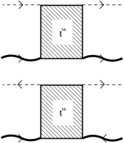
Figure 3: The normal (top) and anomalous (bottom) self energy contributions to the bosonic propagator. The wavy lines are bosonic propagators.

Turning to the bosonic propagator, we find that there are no diagrams contributing to $\Sigma_{11}$ and $\Sigma_{20}$ at the order of $\Delta_{0}$. At the order of $\Delta_{0}^{2}$, the self energy diagrams are shown on Fig 3. The square box denotes the sum of all the diagrams which contribute to the $T$-matrix of scattering of a boson off another boson. Just as those for $t^{\rm bf}$, these diagrams can also be summed up using the appropriate Lippmann-Schwinger equation. We denote the result of summation $t^{\rm bb}$. $t^{\rm bb}$ is calculated in section VI. Thus we find

$$\Sigma_{11}^{(2)}=2\Delta_{0}^{2}t^{\rm bb},\ \Sigma_{20}^{(2)}=\Delta_{0}^{2}t^{\rm bb}.$$ (21)

The coefficient $2$ appears as the appropriate combinatorial factor.

It is also possible to consider diagrams higher order in $\Delta_{0}$ which contribute to the bosonic normal and anomalous self energy. One such diagram, which contributes to $\Sigma_{11}^{(4)}$, is shown on Fig 4. There are infinitely many similar diagrams contributing to $\Sigma^{(4)}_{11}$ and $\Sigma_{20}^{(4)}$. We will not discuss these any further.

Figure 4: A possible higher order contribution to the bosonic self energy.

IV Calculation of the speed of sound and the condensate depletion

Once the self energy terms are known, the procedure for calculating the chemical potential, the speed of sound, and the condensate depletion is fairly standard.

First of all, we calculate the normal and anomalous bosonic Green’s functions $D_{n,a}$, given $\Sigma_{11}$ and $\Sigma_{20}$. The calculation involves solving the appropriate Dyson equation Abrikosov et al. (1977) and the result is

$$D_{n}(p,\omega) = \frac{D_{0}^{-1}(-p,-\omega)-\Sigma_{11}(-p,-\omega)}{D(p,\omega)},$$ (22)

$$D_{a}(p,\omega) = \frac{\Sigma_{20}(p,\omega)}{D(p,\omega)},$$ (23)

where

$$D(p,\omega) = -\left[\Sigma_{20}(p,\omega)\right]^{2}+\left(D_{0}^{-1}(p,\omega)-\Sigma_{11}(p,\omega)\right)\times$$ (25)

$$\times\left(D_{0}^{-1}(-p,-\omega)-\Sigma_{11}(-p,-\omega)\right).$$

The Hugenholtz-Pines relation then takes the form

$$D(0,0)=0.$$ (27)

In the lowest order in density, the self energy terms $\Sigma_{11}$ and $\Sigma_{20}$ vanish. Then the Hugenholtz-Pines relation reads

$$D_{0}^{-1}(0,0)=0.$$ (28)

Recalling the definition of $D_{0}$, Eq. (18), we immediately find $\mu=-1/(2ma^{2})$, the same relation as the one which follows from the gap equation, Eq. (14).

In the first nonvanishing order in density, the self energy terms are given by Eq. (21). We are interested in the self energy at zero momentum and frequency, thus $t^{\rm bb}$ also needs to be computed at zero momentum and frequency. In section VI we show how to calculate $t^{\rm bb}$ in vacuum by solving the appropriate Lippmann-Schwinger equation. We, however, need $t^{\rm bb}$ at a finite chemical potential $\mu$. Fortunately, if

$$\left|\mu+1/(2ma^{2})\right|\ll\left|\mu\right|,$$ (29)

then $t^{\rm bb}$ at a finite $\mu$ is approximately given by its expression computed in vacuum at zero momentum and frequency. In other words, it is proportional to $a_{b}$, where $a_{b}$ is the bosonic scattering length in vacuum, Eq. (2). The Lippmann-Schwinger equation can only be solved numerically, so we only know the numerical value of $a_{b}$.

More precisely, $t^{\rm bb}$ at zero momentum and frequency, and at chemical potential satisfying Eq. (29) is related to the scattering length $a_{b}$ as follows

$$t^{\rm bb}=\frac{2\pi a_{b}}{mZ^{2}},$$ (30)

where $Z$ is the residue of the bosonic propagator $D_{0}$ at its pole, or

$$Z=\frac{8\pi}{m^{2}a}.$$ (31)

We expect Eq. (29) to hold as we expect $\mu$ to deviate only slightly from its zero density value Eq. (14) in the low density approximation employed here.

Armed with these relations, we introduce a bosonic chemical potential

$$\mu_{b}=2\mu+\frac{1}{ma^{2}}$$

and solve the Hugenholtz-Pines relation in the next order in density

$$\mu_{b}=\frac{a\,a_{b}\,m\Delta_{0}^{2}}{4}.$$ (32)

There are actually two solutions of the Hugenholtz-Pines relation, but one of them is well known to be unphysical Abrikosov et al. (1977).

We remark that if we had instead decided to solve the gap equation Eq. (13) by expanding its square root in powers of $\Delta_{0}^{2}$, we would have obtained $\mu_{b}=\Delta_{0}^{2}\,a^{2}m/2$, as if the bosonic scattering length were $a_{b}=2a$. This is manifestly incorrect. Thus we see that the gap equation fails in the BEC regime. In fact, it is easy to see exactly where the gap equation breaks down, and what comes in its place. This analysis is performed in section V.

Now we use the particle number equation Eq. (16) to relate $\Delta_{0}$ to the particle density $n$. Within the lowest approximation in density, we can substitute $\mu=-1/(2ma^{2})$ to find

$$n=\frac{am^{2}\Delta_{0}^{2}}{4\pi}.$$ (33)

Using the next order approximation for the chemical potential would only contribute to the further expansion of Eq. (33) in powers of $\Delta_{0}$, where, however, we would also need to take into account the terms $\Sigma_{a,n}^{(2)}$. Fortunately this is not needed for the calculations in the lowest order presented here.

Combining Eq. (32) and Eq. (33) we find

$$\mu_{b}=\frac{\pi a_{b}n}{m}=\frac{4\pi a_{b}n_{b}}{m_{b}},$$ (34)

where $m_{b}=2m$ is the mass of the bosonic dimers and $n_{b}=n/2$ is their density. This is the first of the results advertised in the beginning of the paper in Eq. (I).

To find the speed of sound, we impose the condition

$$D(p,\omega)=0.$$ (35)

This gives us a relation between $\omega$ and $p$. For small $\omega$ and $p$, with the help of Eq. (33) it reduces to

$$\omega^{2}=p^{2}\frac{4\pi n_{b}a_{b}}{m_{b}^{2}}.$$ (36)

Comparing with $\omega^{2}=u^{2}p^{2}$, where $u$ is the speed of sound, gives the second result in Eq. (I).

Finally, we calculate the condensate depletion. The density of bosons not in the condensate can be calculated as

$$\delta n_{b}=\frac{i}{Z}\lim_{t\rightarrow-0}\int\frac{d\omega\,d^{3}p}{(2\pi)^{4}}~{}D_{n}(p,\omega)\,e^{-i\omega t}.$$ (37)

The calculation of the integral in Eq. (37) demands knowing the full frequency and momentum dependence of the self energy terms $\Sigma_{11}$ and $\Sigma_{20}$. This in principle can only be found numerically, since the knowledge of full frequency and momentum dependence of $t^{\rm bb}$ is required. However, in the limit of small density where self energy terms are small, the relevant frequency and momentum which contribute to the integral in Eq. (37) are in the range $\omega\sim\Delta_{0}^{2}$ and $p^{2}/(4m)\sim\Delta_{0}^{2}$. Thus we expand $D_{0}^{-1}$ in powers of $\Delta_{0}^{2}\sim|\omega+p^{2}/(2m_{b})-\mu_{b}|\ll 1/(ma^{2})$ to find the approximate expression for the free bosonic propagator Eq. (18)

$$\frac{1}{Z}D_{0}(p,\omega)\approx\frac{1}{\omega-\frac{p^{2}}{4m}+\mu_{b}+i0}.$$ (38)

At the same time $Z\Sigma_{20}$ coincides with its expression for the dilute interacting Bose gas. With this substitution, $D_{n}(p,\omega)$ is equal to that of the dilute Bose gas, with the scattering length $a_{b}$. Thus the standard formula for the condensate depletion Abrikosov et al. (1977) holds, and it reads

$$n_{0,b}=n_{b}-\delta n_{b}\approx n_{b}\left[1-\frac{8}{3}\sqrt{\frac{n_{b}\,a_{b}^{3}}{\pi}}\right],$$ (39)

which is the final result in Eq. (I). We emphasize that this is also an expansion in powers of $na^{3}$, and that next order terms will likely depend on the functional dependence of the self energy terms on the frequency and momentum.

Let us summarize what one needs to do to go beyond the lowest order approximation discussed above. The diagrams for the higher order corrections to $\Sigma_{11}$ and $\Sigma_{20}$, such as the one shown on Fig. 4, have to be evaluated. There will be an infinite number of such diagrams, and they can possibly be summed up using a numerical technique similar to the one employed here to calculate $t^{\rm bb}$. One also needs to calculate higher order corrections to $\Sigma_{a}$ and $\Sigma_{n}$. In particular, at the order of $\Delta_{0}^{2}$, $t^{\rm bf}$ has to be evaluated. Because of the nonzero chemical potential present in the external lines of the diagrams shown on Fig. 2, $t^{\rm bf}$ will not reduce simply to the scattering length $a_{bf}$, and so extra work will be needed to find the value of $\Sigma_{n}^{(2)}$. As pointed out by Hugenholtz and Pines in Ref. Hugenholtz and Pines (1959), at each order one also needs to correct the propagators such that a gapless sound mode is produced at this order.

Once the self energy terms are found in the desired order, one needs to solve the Hugenholtz-Pines relation in the next order of $\Delta_{0}^{2}$. This also involves taking into account the dependence of $t^{\rm bb}$ on $\mu_{b}$, which was neglected here due to $\mu_{b}$ being zero up to terms of the order of $\Delta_{0}^{2}$. This allows to find the chemical potential. Given the chemical potential, one can also find corrections to the spectrum by looking at the poles of the propagator. For that, the expansion of $t^{\rm bb}$ in powers of momentum will also be needed. This expansion is also required in order to find corrections to the condensate depletion, given at the lowest order in Eq. (39).

V The origin of the failure of the BCS-BEC gap equation

An alternative method of deriving the results of the previous section is presented here. A convenient way to derive the BCS-BEC gap equation is by shifting $\Delta$ by $\Delta_{0}$ in Eq. (6) and differentiating the resulting $Z$ with respect to $\bar{\Delta}_{0}$, assuming that $\Delta_{0}$ gives an extremum of $\log Z$. This gives

$$-\frac{\Delta_{0}}{\lambda}=\left\langle\,\psi_{\downarrow}\psi_{\uparrow}\,\right\rangle.$$ (40)

To derive the naive gap equation Eq. (13) one usually evaluates the right hand side of Eq. (40) at constant $\Delta=\Delta_{0}$. While this procedure works in the BCS regime, it actually breaks down in the opposite BEC regime.

Indeed, on the BEC side of the crossover, it is more appropriate to expand everything in powers of $\Delta_{0}$. So we instead compute the right hand side of Eq. (40) in terms of diagrams with a fixed number of condensate lines.

The simplest diagram contributing to Eq. (40) is shown on Fig. 5. There are two condensate lines shown on that diagram. The line on the left is not an actual line. Rather it is drawn simply for convenience, and the vertex where it is attached to the diagram represents $\psi_{\downarrow}\psi_{\uparrow}$ whose correlation function we are computing. The line on the right, however, is the actual condensate line. Thus this diagram has one condensate line and is proportional to $\Delta_{0}$.

Figure 5: The simplest diagram contributing to the gap equation Eq. (40).

If we use this diagram for the right hand side of Eq. (40), we derive Eq. (13) with the substitution $\Delta_{0}=0$. Thus this reproduces the lowest order gap equation, and gives Eq. (14) for $\mu$.

This is the only possible diagram with one condensate line. There are no diagrams with two condensate lines either. Once we allow for three external condensate lines, we find one possible diagram shown on Fig. 6.

Figure 6: The simplest diagram contributing to the gap equation at order $\Delta_{0}^{3}$.

This diagram, when taken into account, gives the usual gap equation Eq. (13) where the square root has been expanded up to linear order with respect to $\Delta_{0}^{2}$. We know that solving Eq. (13) at this order gives $a_{b}=2a$ Sá de Melo et al. (1993). And indeed, the diagram shown on Fig. 6 is nothing but the simplest process contributing to the boson-boson $T$-matrix, which is the very first diagram on Fig. 11. In other words, it is the Born approximation for the boson-boson scattering.

We know that the Born approximation breaks down in the BEC regime. Instead, at this order we need to take all the diagrams with three external lines, which are equal to $t^{\rm bb}$, as shown on Fig. 7.

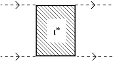
Figure 7: The sum of all diagrams contributing to the gap equation at order $\Delta_{0}^{3}$.

This gives the correct gap equation, with $2a$ being replaced by $0.60\,a$.

To summarize, instead of using the naive gap equation Eq. (13) which does not take into account fluctuations around $\Delta_{0}$, in the BEC regime we use Eq. (40), expanding the right hand side in powers of $\Delta_{0}$. This procedure goes beyond the Born approximation and reproduces the correct results in the BEC regime.

VI Scattering of particles and bound states

Figure 8: Diagrams contributing to the $t$-matrix of fermion-boson scattering.

In this section we consider the scattering of a fermion by a bound state of fermions and scattering between bound states of fermions. All calculations proceed in vacuum so we set $\mu=0$ for this entire section. As argued in section IV, these vacuum scattering processes are precisely those needed to calculate the normal and anomalous fermion self energies at next to leading order in the low density expansion and the lowest order boson normal and anomalous self energies, respectively.

The scattering $t$-matrix consists of all diagrams with incoming and outgoing lines corresponding to the scattering particles. Since we work in vacuum, there is no hole propagation, or all the propagators are retarded. These observations greatly simplify the possible diagrams. In fact, had any of the propagators been advanced, there would be no hope of summing the diagrams contributing to the scattering processes exactly. Fortunately, when all the propagators are retarded, we are able to sum all the diagrams using Lippmann-Schwinger type integral equations. We emphasize that all the calculations proceed in the regime of vanishing effective range $r_{0}$, so the results of this sections are valid only for potentials where $|a|\gg|r_{0}|$.

We first consider scattering of a fermion and a bound state of two fermions, a bosonic dimer. This process was first solved in the zero effective range approximation by Skorniakov and Ter-Martirosian Skorniakov and Ter-Martirosian (1956) in the related problem of neutron-deuteron scattering. We include here a somewhat detailed description of this scattering process in part because it is a useful exercise before considering the more complicated case of scattering between two bosons.

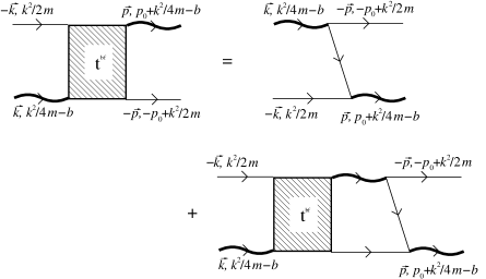
Figure 9: The integral equation for the $t$-matrix of fermion-boson scattering.

The first few diagrams contributing to the $t$-matrix are shown in Fig. 8, where the external lines are not part of the $t$-matrix. Even though all the propagators are retarded, there is still an infinite number of diagrams containing retarded propagators only, and they all contribute at the same order. Indeed, from these first examples it is clear that any such contribution to the $t$-matrix will have $n\geq 0$ boson lines of order $a/m$, see Eq. (18), $2n+1$ fermion lines of order $1/E\sim ma^{2}$ and $n$ integrations of order $Ep^{3}\sim m^{-1}a^{-5}$. Thus each diagram contributing to the $t$-matrix is of order $ma^{2}$.

There is no hope of computing these diagrams one by one and summing them up. Instead, we derive an integral equation which their sum satisfies. Let the incoming boson and fermion have on-shell 4-momenta $(\vec{k},k^{2}/4m-b)$ and $(-\vec{k},k^{2}/2m)$, respectively, and let the outgoing boson and fermion have 4-momenta $(\vec{p},p_{0}+k^{2}/4m-b)$ and $(-\vec{p},-p_{0}+k^{2}/2m)$, respectively. Here $b$ is the binding energy of the dimer, $-1/(ma^{2})\equiv-b$. The $t$-matrix with these kinematics is denoted $t^{\rm bf}_{\vec{k}}(\vec{p},p_{0})$. Then the $t$-matrix satisfies the integral equation

$$t^{\rm bf}_{\vec{k}}(\vec{p},p_{0}) = -G_{0}(\vec{k}+\vec{p},-k^{2}/4m-b+p_{0})$$ (41)

$$-i\int\frac{d^{4}q}{(2\pi)^{4}}t^{\rm bf}_{\vec{k}}(\vec{q},q_{0})D_{0}(\vec{q},k^{2}/4m-b+q_{0})$$

$$\times G_{0}(-\vec{q},\frac{k^{2}}{2m}-q_{0})G_{0}(\vec{p}+\vec{q},p_{0}+q_{0}-\frac{k^{2}}{4m}-b),$$

which is depicted in Fig. 9. The minus sign in front of the right hand side of the equation is due to fermionic anticommutations. The reason for letting outgoing momenta be off-shell is that this makes it possible to solve the integral equation. The on-shell point has $|\vec{k}|=|\vec{p}|$ and $p_{0}=0$. It is possible to integrate out the loop energy on the right hand side in Eq. (41) by noting that $t^{\rm bf}_{\vec{k}}(\vec{q},q_{0})$ is analytic in the upper half plane in $q_{0}$ which can be easily seen by looking at the diagrams contributing to the $t$-matrix. This integration sets $q_{0}=k^{2}/2m-q^{2}/2m$ and we thus set $p_{0}=k^{2}/2m-p^{2}/2m$, to have the same dependence in the $t$-matrix on both sides in the equation. Define $t^{\rm bf}_{\vec{k}}(\vec{p},p_{0}=k^{2}/2m-p^{2}/2m)\equiv t^{\rm bf}_{\vec{k}}(\vec{p})$.

At low energies scattering is dominated by $s$-wave scattering, thus Eq. (41) can be averaged first over directions of $\vec{k}$ and then over directions of $\vec{p}$. The angular average of $t^{\rm bf}_{\vec{k}}(\vec{p})$ is denoted $t^{\rm bf}_{k}(p)$. Then the integral equation for the $t$-matrix of fermion-boson scattering becomes

$$t^{\rm bf}_{k}(p) = \frac{m}{2pk}\ln\frac{p^{2}+pk+k^{2}-mE}{p^{2}-pk+k^{2}-mE}$$ (42)

$$+\frac{1}{\pi}\int^{\infty}_{0}dq\,\frac{q}{p}\ln\frac{q^{2}+qp+p^{2}-mE}{q^{2}-qp+p^{2}-mE}$$

$$\times\frac{t^{\rm bf}_{k}(q)}{a^{-1}-\sqrt{m}\sqrt{-E+3q^{2}/4m}}.$$

Here, $E=3k^{2}/4m-b$ is the total energy which is assumed to be less than zero. To calculate the scattering amplitude each external bosonic leg has to be renormalized by the square root of the residue of the pole of the bosonic propagator at the energy of the bound state, $\sqrt{Z}=\sqrt{8\pi/(m^{2}a)}$, compare with Eq. (31). The external fermionic legs are free propagators and do not have to be renormalized. The scattering amplitude is evaluated on shell and is

$$T^{\rm bf}(k)=Zt^{\rm bf}_{k}(k).$$ (43)

The relationship between the scattering length and the scattering amplitude is

$$T^{\rm bf}(0)=\frac{3\pi}{m}a_{bf}.$$ (44)

Solving Eq. (42) it is found that $a_{bf}\approx 1.18a$.

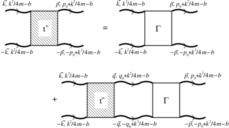
Figure 10: The integral equation for the $t$-matrix of boson-boson scattering. $\Gamma$ is the sum of all two boson irreducible diagrams.

We now turn to the scattering between two bosons where the bosons are bound states of two distinguishable fermions. This process was first solved by Petrov et al Petrov et al. (2005) by solving the quantum mechanical 4-body problem. As we already mentioned, recently, while the work reported here was in progress, the problem was solved in Ref. Brodsky et al. (2005) by using the same diagrammatic approach as we employ below.

As in the case of fermion-boson scattering there are no condensate lines internally in the diagrams and no hole propagation.

Figure 11: The simplest diagrams contributing to the two boson irreducible diagram, $\Gamma$. The first diagram on the right hand side corresponds to $\Gamma^{(0)}$ defined in Eq. (73).

Consider the different diagrams which contribute to the $t$-matrix of boson-boson scattering. The $t$-matrix consists of all possible diagrams with two incoming and two outgoing bosons, the external legs not included. The crucial point is that all of these diagrams are of the same order, namely they are all proportional to $m^{3}a^{3}$ which we will show below. This means that the diagrams contributing to the $t$-matrix do not form a perturbation series and it is not adequate to keep only the Born approximation to the $t$-matrix. Instead an infinite number of diagrams must be taken into account. The summation of all diagrams contributing to the $t$-matrix may be performed by using an integral equation. In particular, the $t$-matrix may be built from a series of two boson irreducible diagrams, which results in an integral equation as shown in Fig. 10. Two boson irreducible diagrams are understood to be diagrams which cannot be cut in half by cutting two boson lines only.

Let the kinematics be as depicted on the figure with the incoming energies and momenta chosen on-shell and the outgoing energies and momenta off-shell to allow for the solution of the integral equation. The on-shell condition is $|\vec{p}|=|\vec{k}|$ and $p_{0}=0$. The $t$-matrix with kinematics as shown on the left hand side of Fig. 10 is denoted by $t^{\rm bb}_{\vec{k}}(\vec{p},p_{0})$. The two boson irreducible diagram with $(\pm\vec{q},E/2\pm q_{0})$ incoming 4-momenta and $(\pm\vec{p},E/2\pm p_{0})$ outgoing 4-momenta is given by $\tilde{\Gamma}_{k}(\vec{q},q_{0};\vec{p},p_{0})$. $E$ is the total energy, $E=-2b+k^{2}/2$. The integral equation corresponding to these kinematics is

$$t^{\rm bb}_{\vec{k}}(\vec{p},p_{0}) = \tilde{\Gamma}_{k}(\vec{k},0;\vec{p},p_{0})$$ (45)

$$+i\int\frac{d^{4}q}{(2\pi)^{4}}D_{0}(\vec{q},E/2+q_{0})D_{0}(-\vec{q},E/2-q_{0})$$

$$\times\tilde{\Gamma}_{k}(\vec{q},q_{0},\vec{p},p_{0})t^{\rm bb}_{\vec{k}}(\vec{q},q_{0}).$$

Thus far the integral equation does not depend on whether the constituents of the dimers are bosons or fermions. Since the scattering is dominated by $s$-wave scattering we average Eq. (45) over directions of $\vec{k}$, then directions of $\vec{p}$ and finally the integration over directions of $\vec{q}$ can be trivially performed. Let the corresponding angular averages be $t^{\rm bb}_{k}(p,p_{0})$ and $\Gamma_{k}(q,q_{0};p,p_{0})$ and let $k\equiv|\vec{k}|$, $p\equiv|\vec{p}|$, and $q\equiv|\vec{q}|$. Then the integral equation becomes

$$t^{\rm bb}_{k}(p,p_{0})=\Gamma_{k}(k,0;p,p_{0})+\frac{4i}{\pi}\int\frac{\Gamma_{k}(q,q_{0};p,p_{0})t^{\rm bb}_{k}(q,q_{0})q^{2}dq\,dq_{0}}{1+\sqrt{(q^{2}/4-E/2)^{2}-q_{0}^{2}}-\sqrt{2}\sqrt{q^{2}/4-E/2+\sqrt{(q^{2}/4-E/2)^{2}-q_{0}^{2}}}},$$ (46)

which contains no remaining angular dependence and where the product of bosonic propagators has been written explicitly using Eq. (18). Since all diagrams are of the same order of magnitude, it is convenient to let all momenta be measured in units of $a^{-1}$ and energies in units of $b=1/(ma^{2})$. $t^{\rm bb}$ and $\Gamma$ are then measured in units of $m^{3}a^{3}$. For simplicity this is the case in Eq. (46) and will be the case in the remainder of this section.

Figure 12: Integral equation for the two boson irreducible diagram with two bosons coming in and one boson and two fermions going out.

The simplest two boson irreducible diagrams are shown in Fig. 11 where the external lines are not a part of $\Gamma$. It is clear that there is an infinite number of such diagrams. Letting $n$ count the number of bosonic propagators in the diagram contributing to $\Gamma$, any such diagram has $4+2n$ fermionic propagators, each of order $ma^{2}$, $n$ bosonic propagators of order $a/m$ and $n+1$ integrations of order $m^{-1}a^{-5}$. Thus each of these diagrams is of order $m^{3}a^{3}$. To see that $t^{\rm bb}$ is also of order $m^{3}a^{3}$ note that any diagram contributing to $t^{\rm bb}$ will contain $n+1$ factors of $\Gamma$, $2n$ bosonic propagators, and $n$ integrations, resulting in any diagram contributing to $t^{\rm bb}$ being proportional to $m^{3}a^{3}$.

Letting the first diagram on the left in Fig. 11 equal the $t$-matrix corresponds to the Born approximation which gives $a_{b}=2a$. Using this same diagram for $\Gamma$ reproduces the result of Ref. Pieri and Strinati (2000), $a_{b}=0.78a$. However in both of these methods an infinite number of diagrams of the same order as those considered is ignored.

The sum of two boson irreducible diagrams may again be obtained through solving an integral equation. The integral equation to be solved is depicted in Fig. 12 where $\Xi$ denotes all two boson irreducible diagrams with two incoming bosons, one outgoing boson and two outgoing fermions. The two boson irreducible diagram $\Gamma$ may then be obtained by tying together the two external fermion lines. Furthermore, since the two boson irreducible diagram $\Gamma$ does not depend on angles, we choose to let $\Xi$ be averaged over the direction of the incoming momentum. Define a four vector $K\equiv(\vec{0},E/2)$ which describes the incoming energy carried by a boson. Then the integral equation corresponding to the kinematics shown on the figure is

$$\Xi_{k}(q,p_{1},p_{2}) = -\int\frac{d\Omega_{\vec{q}}}{4\pi}\left[G_{0}\left(\frac{K}{2}+q-p_{1}\right)G_{0}\left(\frac{K}{2}-q-p_{2}\right)+G_{0}\left(\frac{K}{2}+q-p_{2}\right)G_{0}\left(\frac{K}{2}-q-p_{1}\right)\right]$$ (47)

$$-i\int\frac{d^{4}Q}{(2\pi)^{4}}G_{0}\left(\frac{K}{2}+Q\right)G_{0}\left(\frac{K}{2}-Q-p_{1}-p_{2}\right)\left[\Xi_{k}(q,p_{1},Q)D_{0}(K-Q-p_{1})+\Xi_{k}(q,Q,p_{2})D_{0}(K-Q-p_{2})\right].$$

The minus signs in front of both the first order terms and the higher order terms are a result of anti-commuting fermions. The integral over $d\Omega_{\vec{q}}$ is the averaging over angles of incoming momentum. $\Gamma$ is then found from $\Xi$ by connecting the outgoing fermion lines and integrating over the loop momentum. The precise relation between $\Gamma$ and $\Xi$ is

$$\Gamma_{k}(q;p) = \frac{i}{2}\int\frac{d^{4}q^{\prime}}{(2\pi)^{4}}G_{0}(K/2+q^{\prime})G_{0}(K/2+p-q^{\prime})$$ (48)

$$\times\Xi_{k}(q,q^{\prime},p-q^{\prime}).$$

It is not essential to include both lowest order contributions to $\Xi$ in Eq. (47), the only difference if only one of these were included is that then the factor $1/2$ in Eq. (48) should be removed. However, the symmetric structure of Eq. (47) means that

$$\Xi_{k}(q,p_{1},p_{2})=\Xi_{k}(q,p_{2},p_{1})$$ (49)

which will be useful in the solution of these equations. How we solve the set of equations (46),(47), and (48) is described in detail in Appendix C.

As in the case of fermion-boson scattering, to calculate the scattering amplitude each external bosonic leg has to be renormalized by $\sqrt{Z}=\sqrt{8\pi/(m^{2}a)}$. The scattering amplitude is then evaluated on shell

$$T^{\rm bb}(k)=Z^{2}t^{\rm bb}_{k}(k,0).$$ (50)

with $k\equiv|\vec{k}|$. Here units are restored to the $t$-matrix. The scattering amplitude is related to the boson-boson scattering length by

$$T^{\rm bb}(0)=\frac{2\pi}{m}a_{b}.$$ (51)

By solving Eq. (46) using the method described above and in Appendix C we find $a_{b}\approx 0.60a$ in complete agreement with Refs. Petrov et al. (2005); Brodsky et al. (2005).

Using the above formalism it may also be checked that there are no bound states of a pair of bosons. If such bound states exist, the interaction between the bosons in this theory can become effectively attractive, rendering the bosonic gas unstable. A bound state of two bosons would correspond to a pole in the scattering amplitude, that is, to a solution of the homogenous version of the integral equation (45) for the $t$-matrix. Varying the total energy, that is $k^{2}$ for $k^{2}\leq 0$, we do not find any solutions to the homogenous equation and thus do not find any bound states.

It should be mentioned that the interaction between bosons does not have to be renormalized, in contrast to the interaction between bound states of bosons Efimov (1971). In the latter case, the interaction between a boson and a dimer of bosons depends on the ultraviolet cutoff and a possible solution to this difficulty is to add a three body force counterterm to the theory and use an additional input, such as an experimentally measured three body scattering length Bedaque et al. (1999). However, this difficulty is absent in the case of scattering between a fermion and a dimer of fermions and also in the problem of scattering between two dimers of fermions.

VII Conclusion

In this paper we discussed the low density expansion of the BCS-BEC condensate in the BEC regime. We found the dispersion of its Bogoliubov modes (the speed of sound), its chemical potential, and the condensate depletion in the lowest order approximation in powers of the gas parameter $an^{\frac{1}{3}}$. Notice that the gas parameter increases as the system is tuned towards the BCS-BEC crossover regime, eventually reaching infinity at the so-called unitary point lying in between the BCS and BEC condensate. So the theory developed here works in the BEC regime only and breaks down in the crossover area.

Throughout the paper we emphasized that the BCS-BEC gap equation actually breaks down in the BEC regime. We would like to remark further on the origin of this breakdown. The gap equation is derived by minimizing the effective action of the condensate, given by Eq. (10). This is correct only if the fluctuations about this minimum are small. If they are not small, the fluctuations must be taken into account. In that case, minimization of the effective action should be replaced by minimization of the effective potential, which takes into account fluctuations, as discussed in any textbook on field theory. In practice, it is possible to replace the evaluation of the minimum of the effective potential by the Hugenholtz-Pines relation, as is done here. The advantage of this second procedure is in the fact that it automatically gives the excitation spectrum in addition to the chemical potential. The two techniques are however equivalent. Most importantly, the calculations performed in this paper demonstrate that in including the fluctuations into the effective potential, one needs to go well beyond the Gaussian fluctuations approximation. In fact, terms up to infinite order (in terms of the number of loops) have to be summed up, all of them being of the same order in the gas parameter. Fortunately, this is possible to do, and this is what has been accomplished in this paper. Alternatively, the gap equation corrected by fluctuations was calculated in section V. We demonstrated how the naive gap equation breaks down due to fluctuations, and how the fluctuations effectively replace the Born approximation with the full boson-boson scattering amplitude. If we wanted, we could follow the procedure outlined in section V as an alternative to the Hugenholtz-Pines relation.

The same argument also demonstrates that the Gross-Pitaevskii equation of the condensate should follow not from the effective action, but from the effective potential. In other words, the true bosonic scattering length Eq. (2) should be used in its quartic term, as opposed to its Born approximation value $2a_{b}$. The Gross-Pitaevskii equation will of course be valid only at length scales much bigger than $a$.

All calculations in this paper are done in the lowest approximation in density, which significantly simplifies the work needed to be done. Finding higher order corrections to Eq. (I) is one possible direction of further work along the lines discussed in this paper. Another possible direction is to study the condensate at finite temperature. This should probably be done in the large $N$ approximation such as the one used in Ref. Baym et al. (2000). Generalizing the techniques of our paper to finite temperature should be a promising direction of further research.

On the other hand, we do not expect that these techniques will help to shed light on the BCS-BEC crossover regime, especially at the unitary point. The small parameter utilized here becomes infinity there. The unitary regime can only be understood numerically Bulgac et al. (2006), barring an invention of an exact solution.

Appendix A The Two channel model

The two channel model is defined by its functional integral

$$Z=\int{\cal D}\bar{\psi}_{\uparrow}{\cal D}\psi_{\uparrow}{\cal D}\bar{\psi}_{\downarrow}{\cal D}\psi_{\downarrow}{\cal D}b{\cal D}\bar{b}~{}e^{iS_{\rm tc}},$$ (52)

where the action $S_{\rm tc}$ is given by $S_{\rm tc}=S_{0}+S_{0b}+S_{ab}$. Here $S_{0}$ is the free fermion action given in Eq. (4). $S_{0b}$ is the free boson action given by

$$S_{0b}=\int d^{3}x~{}dt~{}\bar{b}\left(i\frac{\partial}{\partial t}+\frac{1}{4m}\frac{\partial^{2}}{\partial{\bf x}^{2}}+2\mu-\epsilon_{0}\right)b,$$ (53)

where $\epsilon_{0}$ is the detuning, the parameter controlled by the magnetic field in the Feshbach resonance setup. $S_{ab}$ is the interaction term

$$S_{ab}=-g\int d^{3}x~{}dt~{}\left(b\,\bar{\psi}_{\uparrow}\bar{\psi}_{\downarrow}+\bar{b}\,\psi_{\downarrow}\psi_{\uparrow}\right).$$ (54)

The scattering of fermions in the two channel model is characterized by the scattering length $a$ and effective range $r_{0}$ given by Andreev et al. (2004)

$$a=-\frac{mg^{2}}{4\pi\left(\epsilon_{0}-\frac{g^{2}m\Lambda}{2\pi^{2}}\right)},\ r_{0}=-\frac{8\pi}{m^{2}g^{2}}.$$ (55)

In order to ensure that we work in the wide resonance regime $|r_{0}|\ll n^{-{\frac{1}{3}}}$, $|r_{0}|\ll|a|$, in this paper we need to take the limit $g\rightarrow\infty$, while simultaneously adjusting $\epsilon_{0}$ so that $a$ remains finite. Introducing the notation $\Delta=gb$, $\bar{\Delta}=g\bar{b}$, we find that $g$ disappears from $S_{ab}$, while $S_{0b}$, in the large $g$ limit, becomes

$$S_{0b}=\left(\frac{m}{4\pi a}-\frac{m\Lambda}{2\pi^{2}}\right)\int d^{3}xdt\,\bar{\Delta}\Delta.$$ (56)

We recognize the combination of parameters in brackets as $-1/\lambda$, thanks to Eq. (12). Thus the two channel model reduces to the one channel model as given by Eq. (4) and Eq. (7).

One important lesson which follows from this discussion is that in the wide resonance regime, it is not justified to use $g$ as a small parameter and construct perturbative expansion in its powers. Indeed, $g$ is not only not small, it should actually be taken to infinity.

Appendix B Fermionic Scattering and renormalized bosonic propagator

Figure 13: The bubble diagrams of fermion scattering.

The scattering of fermions governed by the action Eq. (4) and interacting via the short range interaction Eq. (5) can be calculated by summing up the diagrams depicted in Fig. 13. The calculation proceeds in vacuum, so the chemical potential $\mu$ is set to zero everywhere. This sum gives the fermion $T$-matrix, $T^{\rm ff}$, and the scattering length is proportional to the $T$-matrix at zero momentum,

$$a=\frac{m}{4\pi}T^{\rm ff}(0).$$ (57)

The bubble diagrams form a geometric series which can be summed to give

$$T^{\rm ff}(0)=\frac{-\lambda}{1+\lambda\Pi(0)}$$ (58)

where $\Pi$ is a bubble as shown in Fig. 13 evaluated at zero momentum. This bubble is given by

$$\Pi(0)=i\int\frac{d^{4}p}{(2\pi)^{4}}G_{0}(p)G_{0}(-p)\\ =-\frac{m\Lambda}{2\pi^{2}}.$$

Here, $\Lambda$ is the momentum cut-off. This shows Eq. (12), namely that

$$a=\left(-\frac{4\pi}{m\lambda}+\frac{2\Lambda}{\pi}\right)^{-1}.$$ (59)

Figure 14: The bosonic propagator renormalized by fermion loops. The thin wavy lines are unrenormalized boson propagators.

The calculation of the bosonic propagator corrected by fermionic loops proceeds similarly. Having in mind its applications in this paper, we do this calculation at a finite chemical potential $\mu\leq 0$. Expanding the action $S_{\Delta}$ in Eq. (10) results in a geometric series as shown in Fig. 14, which can be summed to give

$$D_{0}(p)=\frac{-\lambda}{1+\lambda\Pi(p)}.$$ (60)

The fermion loop can be calculated to give

$$\Pi(p) = i\int\frac{d^{4}q}{(2\pi)^{4}}G_{0}(p+q)G_{0}(-q)$$ (61)

$$=-\frac{m\Lambda}{2\pi^{2}}+\frac{m^{3/2}}{4\pi}\sqrt{-\omega+p^{2}/4m-2\mu-i0}.$$

Inserting this result in Eq. (60), using Eq. (12) to write the momentum cut-off in terms of $a$, finally gives

$$D_{0}(p)=\frac{4\pi}{m}\frac{1}{a^{-1}-\sqrt{m}\sqrt{-\omega+\frac{p^{2}}{4m}-2\mu-i0}}.$$ (62)

Note that it is crucial that $\mu\leq 0$ for the integral in Eq. (61) to be calculated the way it is. Otherwise, the fermionic propagator is no longer retarded due to hole propagation. Thus Eq. (62) applies only in vacuum or in the BEC regime where $\mu\leq 0$.

Appendix C The integral equation for boson-boson scattering

In this appendix we describe the solution of Eqs. (46-48), describing scattering of two bound states, each consisting of two fermions. We demonstrate how to integrate out the loop energies in constructing the sum of two boson irreducible diagrams, $\Gamma$, and we write the corresponding equations in a more convenient way for numerical studies. We also describe the numerical methods used. For simplicity, in this appendix all momenta are measured in units of $a^{-1}$, all energies in units of $1/(ma^{2})$, and $t^{\rm bb}$ and $\Gamma$ in units of $m^{3}a^{3}$.

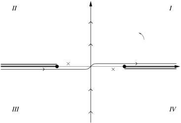
Figure 15: The original and rotated contours of frequency integration used in Eq. (46). The crosses correspond to poles of the bosonic propagators which approach the imaginary axis as $k,q\to 0$. The dots and black lines towards $\pm\infty$ are branch cuts of the bosonic propagators and the grey boxes are possible non-analytic structure of $\Gamma(q,q_{0};p,p_{0})$. These do not come closer to the imaginary axis than $\pm b$.

To construct $\Gamma_{k}(q,q_{0};p,p_{0})$ it is convenient first to rotate the external energies $p_{0}$ and $q_{0}$ onto the imaginary axis which can be done without crossing any poles. Both applications we have in mind, calculation of the scattering length and search for bound states, require the $t$-matrix $t^{\rm bb}_{k}(p,p_{0})$ evaluated on shell and thus we are only interested in the $t$-matrix evaluated at $p_{0}=0$ which is still on the contour. That it is possible to rotate the external energies is not immediately obvious. Consider Eq. (46) which relates the $t$-matrix to $\Gamma$. The two bosonic propagators have branch cuts in $q_{0}$ starting at $q_{0}=\pm(1+q^{2}/4-k^{2}/4)$ and going towards $\pm\infty$, respectively. $1+q^{2}/4-k^{2}/4>0$ since to calculate the scattering length we let $k=0$ and to search for bound states we let $k^{2}\leq 0$. The bosonic propagators also have poles at $q_{0}=\pm(q^{2}/4-k^{2}/4-i0)$ where the infinitesimal is determined from the requirement that Eq. (18) describes a retarded propagator. It will be shown below that also $\Gamma(q,q_{0};p,p_{0})$ can only be non-analytic in quadrant $II$ above the branch cut and $IV$ below the branch cut in $p_{0}$ and $q_{0}$. We conclude that not only is it possible to rotate the external energies, but we also move the contour of integration away from any singularities. This is illustrated in Fig. 15. The only remaining singularities close to the integration contour are from the poles of the bosonic propagator as $q\to 0$ and $k\to 0$. This singularity is integrable and we will explicitly treat this below by a change of variables in Eq. (74).

In the integral equation (47) it is possible to integrate over the loop energy since $\Xi_{k}(q,p_{1},p_{2})$ is analytic in the lower half planes of both fermion energies. To see this, note that for any diagram contributing to $\Xi$ the two outgoing fermionic propagators do not originate from the same bosonic propagator since then $\Xi$ would be two boson reducible. Instead each of the fermions originate from a boson which in turn decays into one other fermion which through a series of propagations forward in time contribute to the creation of the outgoing boson. Thus $\Xi$ contains only retarded propagators of $-p_{1}$ and $-p_{2}$ and must be analytic in the lower half planes of the corresponding energies.

It is not as simple to integrate out the loop energy in Eq. (48) since $\Xi_{k}(q,q^{\prime},p-q^{\prime})$ is not analytic in either $q^{\prime}_{0}$ half planes. However, if one considers the integral equation satisfied by $\Xi_{k}(q,q^{\prime},p-q^{\prime})$, Eq. (47) with $p_{1}=q^{\prime}$ and $p_{2}=p-q^{\prime}$, the first product of propagators can be split into a term analytic in the upper $q^{\prime}_{0}$ half plane and a term analytic in the lower $q^{\prime}_{0}$ half plane by noting that

$$G_{0}(K/2+q-q^{\prime})G_{0}(K/2-q-p+q^{\prime})$$

$$=\frac{G_{0}(K/2+q-q^{\prime})+G_{0}(K/2-q-p+q^{\prime})}{\frac{E}{2}-p_{0}-(\vec{q}-\vec{q}\,^{\prime})^{2}/2-(\vec{q}+\vec{p}-\vec{q}\,^{\prime})^{2}/2+i0}.$$ (63)

The second product of fermionic propagators is treated similarly. The remaining part of the integral equation for $\Xi_{k}(q,q^{\prime},p-q^{\prime})$ consists of a term analytic in the upper $q^{\prime}_{0}$ half plane and a term analytic in the lower $q^{\prime}_{0}$ half plane. Thus effectively we have split $\Xi_{k}(q,q^{\prime},p-q^{\prime})$ into

$$\Xi_{k}(q,q^{\prime},p-q^{\prime})=\Xi^{+}_{k}(q,q^{\prime},p-q^{\prime})+\Xi^{-}_{k}(q,q^{\prime},p-q^{\prime})$$ (64)

with $\Xi^{+}_{k}(q,q^{\prime},p-q^{\prime})$ ($\Xi^{-}_{k}(q,q^{\prime},p-q^{\prime})$) analytic in the upper (lower) $q_{0}^{\prime}$ half plane. Note that this splitting means that in complete generality

$$\Xi_{k}(q,p_{1},p_{2})=\Xi^{+}_{k}(q,p_{1},p_{2})+\Xi^{-}_{k}(q,p_{1},p_{2}).$$ (65)

$\Xi^{+}_{k}(q,q^{\prime},p-q^{\prime})$ and $\Xi^{-}_{k}(q,q^{\prime},p-q^{\prime})$ satisfy a set of coupled integral equations. The equation satisfied by $\Xi^{-}_{k}(q,q^{\prime},p-q^{\prime})$ is

$$\Xi^{-}_{k}(q,q^{\prime},p-q^{\prime})=$$

$$-\int\frac{d\Omega_{\vec{q}}}{4\pi}\left[\frac{G_{0}(K/2+q-q^{\prime})}{\frac{E}{2}-p_{0}-(\vec{q}-\vec{q}\,^{\prime})^{2}/2-(\vec{q}+\vec{p}-\vec{q}\,^{\prime})^{2}/2+i0}+\frac{G_{0}(K/2-q-q^{\prime})}{\frac{E}{2}-p_{0}-(\vec{q}+\vec{q}\,^{\prime})^{2}/2-(\vec{q}-\vec{p}+\vec{q}\,^{\prime})^{2}/2+i0}\right]$$

$$-\left.\int\frac{d^{3}Q}{(2\pi)^{3}}G_{0}(K/2-Q-p)D_{0}(K-Q-q^{\prime})\Xi_{k}(q,q^{\prime},Q)\right|_{Q_{0}=\vec{Q}^{2}/2-E/4}.$$ (66)

The right hand side of this equation is related to $\Xi^{+}$ through Eq. (65). The crucial point is that the right hand side of Eq. (66) equals $\Xi^{+}_{k}(q,p-q^{\prime},q^{\prime})$ which can be seen by writing the corresponding equation for $\Xi^{+}_{k}(q,q^{\prime},p-q^{\prime})$ and using the change of variables $p-q^{\prime}\leftrightarrow q^{\prime}$ along with Eq. (49). Thus $\Xi^{+}_{k}(q,p-q^{\prime},q^{\prime})=\Xi^{-}_{k}(q,q^{\prime},p-q^{\prime})$. Consequently, using Eq. (48), we conclude that $\Xi^{+}_{k}(q,q^{\prime},p-q^{\prime})$ and $\Xi^{-}_{k}(q,q^{\prime},p-q^{\prime})$ has identical contributions to $\Gamma$. We also note that

$$\Xi_{k}(q,p_{1},p_{2})=\Xi^{-}_{k}(q,p_{1},p_{2})+\Xi^{-}_{k}(q,p_{2},p_{1}),$$ (67)

which may be inserted in the right hand side of Eq. (66). The result is an un-coupled integral equation for $\Xi^{-}_{k}(q,q^{\prime},p-q^{\prime})$.

We now perform the $q^{\prime}_{0}$-integration in the lower half plane in Eq. (48) using Eq. (67). This integration sets $q^{\prime}_{0}=\vec{q}\,^{\prime 2}/2-E/4>0$. At this value of the total outgoing fermion energy Eq. (66) reduces to

$$\Xi_{k}^{-}(q;\vec{q}\,^{\prime},\vec{q}\,^{\prime 2}/2-E/4;\vec{p}-\vec{q}\,^{\prime},p_{0}-\vec{q}\,^{\prime 2}/2+E/4)$$ (68)

$$= \int\frac{d\Omega_{\vec{q}}}{4\pi}\left[\frac{G_{0}(K/2+q-q^{\prime})}{p_{0}+(\vec{q}-\vec{q}\,^{\prime})^{2}/2+(\vec{q}+\vec{p}-\vec{q}\,^{\prime})^{2}/2-E/2-i0}+\frac{G_{0}(K/2-q-q^{\prime})}{p_{0}+(\vec{q}+\vec{q}\,^{\prime})^{2}/2+(-\vec{q}+\vec{p}-\vec{q}\,^{\prime})^{2}/2-E/2-i0}\right]$$

$$+\frac{1}{2\pi^{2}}\int d^{3}Q\,\frac{\Xi^{-}_{k}(q;\vec{q}\,^{\prime},\vec{q}\,^{\prime 2}/2-E/4;\vec{Q},\vec{Q}/2-E/4)+\Xi^{-}_{k}(q;\vec{Q},\vec{Q}/2-E/4;\vec{q}\,^{\prime},\vec{q}\,^{\prime 2}/2-E/4)}{\left(p_{0}+\vec{Q}^{2}/2+(\vec{p}+\vec{Q})^{2}/2-E/2-i0\right)\left(1-\sqrt{-E+3\vec{Q}^{2}/4+3\vec{q}\,^{\prime 2}/4+\vec{Q}\cdot\vec{q}\,^{\prime}/2}\right)}.$$

The right hand side of this equation only contains $\Xi^{-}$ evaluated at fermion energies related to the corresponding momentum by $Q_{0}=\vec{Q}^{2}-E/4$ and $q^{\prime}_{0}=\vec{q}\,^{\prime 2}/2-E/4$, which we will call “on shell”. We will solve the integral equation by first letting

$$p_{0}\to\vec{p}\,^{2}/2+\vec{q}\,^{\prime 2}-\vec{p}\cdot\vec{q}\,^{\prime}-E/2,$$ (69)

which means that the left hand side is also evaluated “on shell”. The resulting integral equation is an integral equation in $|\vec{q}^{\prime}|$, $|\vec{p}-\vec{q}\,^{\prime}|$, and the angle between these, using $|\vec{k}|$, $|\vec{p}|$, $|\vec{q}|$, and $q_{0}$ as input. Subsequently the “on shell” $\Xi^{-}$ can be inserted in the right hand side of Eq. (68) to evaluate $\Xi^{-}$ at any values of the outgoing energy.

It is now possible to conclude that $\Gamma(q,q_{0};p,p_{0})$ is analytic in quadrant $I$ and $III$ in $p_{0}$ and $q_{0}$ and that furthermore any non-analyticity is far from the rotated contour of integration. The remaining pole of a fermionic propagator in Eq. (48) after the $q_{0}^{\prime}$ integration in the lower half plane is at $p_{0}=1-k^{2}/4+\vec{q}\,^{\prime 2}/2+(\vec{p}-\vec{q}\,^{\prime})^{2}/2-i0$ where the real part is greater than $1-k^{2}/4\geq 1$. In Eq. (68) the poles in $p_{0}$ are in quadrant $II$ and also has real part less than $-1+k^{2}/4\leq-1$. Finally, also in Eq. (68), the pole in $q_{0}$ is in quadrant $IV$ below the branch cut.

We now define the “on shell” function

$$\tilde{\Xi}_{k}(q;p_{1},p_{2},\cos\theta) \equiv$$ (70)

$$\Xi^{-}_{k}(q;\vec{p}_{1},\vec{p}_{1}\,^{2}/2-E/4;\vec{p}_{2},\vec{p}_{2}\,^{2}-E/4).$$

Here, $p_{1,2}\equiv|\vec{p}_{1,2}|$ and $\theta$ is the angle between these vectors. We then find the final set of equations to be solved to construct $\Gamma$:

$$\tilde{\Xi}_{k}(q;p_{1},p_{2},\cos\theta) = -\int\frac{d\Omega_{\vec{q}}}{4\pi}\left[\frac{1}{q^{2}+p_{1}^{2}+p^{2}_{2}-\vec{q}\cdot\vec{p}_{1}+\vec{q}\cdot\vec{p}_{2}-E}\frac{1}{-q_{0}+p_{1}^{2}/2+(\vec{q}-\vec{p}_{1})^{2}/2-E/2}\right.$$ (71)

$$\left.+\frac{1}{q^{2}+p_{1}^{2}+p^{2}_{2}+\vec{q}\cdot\vec{p}_{1}-\vec{q}\cdot\vec{p}_{2}-E}\frac{1}{q_{0}+p_{1}^{2}/2+(\vec{q}+\vec{p}_{1})^{2}/2-E/2}\right]$$

$$+\frac{1}{\pi}\int_{-1}^{1}d(\cos\phi)\int_{0}^{\infty}Q^{2}dQ\frac{1}{1-\sqrt{-E+3Q^{2}/4+3p_{1}^{2}/4+Qp_{1}\cos\phi/2}}$$

$$\times\frac{\tilde{\Xi}_{k}(q,p_{1},Q,\cos\phi)+\tilde{\Xi}_{k}(q;Q,p_{1},\cos\phi)}{\sqrt{(Q^{2}+p_{1}^{2}+p_{2}^{2}+Qp_{1}\cos\phi+p_{1}p_{2}\cos\theta+Qp_{2}\cos\theta\cos\phi-E)^{2}-Q^{2}p_{2}^{2}(1-\cos^{2}\theta)(1-\cos^{2}\phi)}}.$$

We now insert Eq. (71) in the right hand side of Eq. (68) using Eq. (70), and subsequently Eq. (68) in Eq. (48). Performing the integral over the azimuthal angle in the $\vec{Q}$ integral we find

$$\Gamma_{k}(q,q_{0};p,p_{0}) = \Gamma_{k}^{(0)}(q,q_{0};p,p_{0})+\frac{1}{4\pi^{3}}\int_{-1}^{1}d(\cos\theta)\int_{0}^{\infty}\frac{q^{\prime 2}dq^{\prime}}{p_{0}-q^{\prime 2}-p^{2}/2+pq^{\prime}\cos\theta+E/2}$$ (72)

$$\times\int_{-1}^{1}d(\cos\phi)\int_{0}^{\infty}\frac{Q^{2}dQ}{1-\sqrt{-E+3Q^{2}/4+3q^{\prime 2}/4+Qq^{\prime}\cos\phi/2}}$$

$$\times\frac{\tilde{\Xi}_{k}(q;q^{\prime},Q,\cos\phi)+\tilde{\Xi}_{k}(q;Q,q^{\prime},\cos\phi)}{\sqrt{(Q^{2}+p^{2}/2+Qp\cos\theta\cos\phi+p_{0}-E/2)^{2}-Q^{2}p^{2}(1-\cos^{2}\theta)(1-\cos^{2}\phi)}},$$

where $\Gamma^{(0)}$ is the contribution from the first diagram on the right hand side in Fig. 11, which can be found to be

$$\Gamma_{k}^{(0)}(q,q_{0};p,p_{0}) = \frac{1}{16\pi^{2}}\int_{0}^{\infty}\frac{dq^{\prime}}{pq}\frac{1}{-E/2+q^{\prime 2}+p^{2}/4+q^{2}/4}\ln\frac{-q_{0}^{2}+(-E/2+q^{\prime 2}+p^{2}/4+q^{2}/4-q^{\prime}p)^{2}}{-q_{0}^{2}+(-E/2+q^{\prime 2}+p^{2}/4+q^{2}/4+q^{\prime}p)^{2}}$$ (73)

$$\times\ln\frac{-p_{0}^{2}+(-E/2+q^{\prime 2}+p^{2}/4+q^{2}/4-q^{\prime}q)^{2}}{-p_{0}^{2}+(-E/2+q^{\prime 2}+p^{2}/4+q^{2}/4+q^{\prime}q)^{2}}.$$

With the energies rotated to the imaginary axis all equations used to find the $t$-matrix, Eq. (46) at $dq_{0}\to i\,dq_{0}$, and Eqs. (71-73) are real. This is not immediately obvious but may be easily checked numerically.

To treat the poles in Eq. (46) of the bosonic propagators at $q_{0}=\pm(q^{2}/4-k^{2}/4-i0)$ as $k,q\to 0$ we perform the following change of variables on the external energies and momenta to “polar” coordinates

$$q^{2}/4 = R^{2}_{1}\cos\theta_{1},\hskip 28.45274ptq_{0}=R_{1}^{2}\sin\theta_{1},$$

$$p^{2}/4 = R^{2}_{2}\cos\theta_{2},\hskip 28.45274ptp_{0}=R_{2}^{2}\sin\theta_{2},$$ (74)

where $R_{i}\in[0,\infty[$ and $\theta_{i}\in[0,\pi/2]$. Here we restrict the integration over $q_{0}$ to the upper imaginary axis, using the symmetry of the integrand in Eq. (46) as $q_{0}\to-q_{0}$. This symmetry follows from the symmetry of the problem. For convergence reasons it is advantageous to integrate over finite intervals, and to this end we use the change of variables

$$R_{i}=\frac{2}{z_{i}+1}-1.$$ (75)

We employ the same change of variables on the internal loop momenta $Q$ and $q^{\prime}$ in Eqs. (71) and (72),

$$Q=\frac{2}{z_{Q}+1}-1,\,\,\,q^{\prime}=\frac{2}{z^{\prime}+1}-1.$$ (76)

To solve the integral equations (46) and (71) we use the Nystrom method, writing the integral equations as matrix equations and inverting these to find the solution. Evaluation of the integrals in these integral equations is performed using Gauss-Legendre quadrature Press et al. (1996).

References

- Leggett (1980) A. Leggett, in Modern Trends in the Theory of Condensed Matter (Springer-Verlag, Berlin, 1980), pp. 13–27.
- Nozières and Schmitt-Rink (1985) P. Nozières and S. Schmitt-Rink, J. Low Temp. Phys. 59, 195 (1985).
- Popov (1966) V. N. Popov, Zh. Eksp. Teor. Phys. 50, 1550 (1966), [Sov. Phys. JETP 23, 1034 (1966)].
- Eagles (1969) D. M. Eagles, Phys. Rev. 186, 456 (1969).
- Timmermans et al. (1999) E. Timmermans, P. Tommasini, M. Hussein, and A. Kerman, Physics Reports 315, 199 (1999).
- Rumer (1959) Y. B. Rumer, Zh. Eksp. Teor. Phys. 37, 578 (1959).
- Holland et al. (2001) M. Holland, S. J. J. M. F. Kokkelmans, M. L. Chiofalo, and R. Walser, Phys. Rev. Lett. 87, 120406 (2001).
- Timmermans et al. (2001) E. Timmermans, K. Furuya, P. W. Milonni, and A. K. Kerman, Phys. Lett. A 285, 228 (2001).
- Strecker et al. (2003) K. E. Strecker, G. B. Partridge, and R. G. Hulet, Phys. Rev. Lett. 91, 080406 (2003).
- Regal et al. (2004) C. A. Regal, M. Greiner, and D. S. Jin, Phys. Rev. Lett. 92, 040403 (2004).
- Zwierlein et al. (2004) M. W. Zwierlein, C. A. Stan, C. H. Schunck, S. M. F. Raupach, A. J. Kerman, and W. Ketterle, Phys. Rev. Lett. 92, 120403 (2004).
- Petrov et al. (2005) D. S. Petrov, C. Salomon, and G. V. Shlyapnikov, Phys. Rev. A 71, 012708 (2005).
- Abrikosov et al. (1977) A. A. Abrikosov, L. P. Gorkov, and I. E. Dzyaloshinski, Methods of Quantum Field Theory in Statistical Physics (Dover Publications, Cambridge, UK, 1977).
- Andersen (2004) J. O. Andersen, Rev. Mod. Phys. 76, 599 (2004).
- Gurarie and Radzihovsky (2005) V. Gurarie and L. Radzihovsky, in preparation (2005).
- Brodsky et al. (2005) I. V. Brodsky, M. Y. Kagan, A. V. Klaptsov, R. Combescot, and X. Leyronas, JETP Letters 82, 273 (2005).
- Keldysh and Kozlov (1968) L. V. Keldysh and A. N. Kozlov, Zh. Eksp. Teor. Phys. 54, 978 (1968), [Sov. Phys. JETP 27, 521 (1968)].
- Sá de Melo et al. (1993) C. A. R. Sá de Melo, M. Randeria, and J. R. Engelbrecht, Phys. Rev. Lett. 71, 3202 (1993).
- Hugenholtz and Pines (1959) N. M. Hugenholtz and D. Pines, Phys. Rev. 116, 489 (1959).
- Skorniakov and Ter-Martirosian (1956) G. V. Skorniakov and K. A. Ter-Martirosian, Zh. Eksp. Teor. Phys. 31, 775 (1956), [Sov. Phys. JETP 4, 648 (1957)].
- Pieri and Strinati (2000) P. Pieri and G. C. Strinati, Phys. Rev. B 61, 15370 (2000).
- Efimov (1971) V. N. Efimov, Sov. J. Nucl. Phys. 12, 589 (1971).
- Bedaque et al. (1999) P. F. Bedaque, H.-W. Hammer, and U. van Kolck, Nucl.Phys. A 646, 444 (1999).
- Baym et al. (2000) G. Baym, J.-P. Blaizot, and J. Zinn-Justin, Europhys. Lett. 49, 150 (2000).
- Bulgac et al. (2006) A. Bulgac, J. E. Drut, and P. Magierski, Phys. Rev. Lett. 96, 090404 (2006).
- Andreev et al. (2004) A. V. Andreev, V. Gurarie, and L. Radzihovsky, Phys. Rev. Lett. 93, 130402 (2004).
- Press et al. (1996) W. H. Press, S. A. Teukolsky, W. T. Vetterling, and B. P. Flannery, Numerical Recipes in Fortran 77: The Art of Scientific Computing (Cambridge University Press, Cambridge, 1996).