Inversion techniques for optical conductivity data

Abstract

Optical data is encoded with information on the microscopic interaction between charge carriers. For an electron-phonon system, the Eliashberg equations apply and a Kubo formula can be used to get the infrared conductivity. The task of extracting the electron-phonon spectral density $\alpha^{2}F(\omega)$ from data is rather complicated and, thus, simplified but approximate expressions for the conductivity have often been used. We test the accuracy of such simplifications and also discuss the advantages and disadvantages of various numerical methods needed in the inversion process. Normal and superconducting state are considered as well as boson exchange mechanisms which might be applicable to the High-$T_{c}$ oxides.

I Introduction

The interaction Hamiltonian between electrons and phonons involves a complicated matrix element or coupling function $g_{{\bf k},{\bf k}^{\prime},\nu}$ which describes the scattering of an electron initially in the state $|{\bf k}\rangle$ to any final state $|{\bf k}^{\prime}\rangle$ through the exchange of a phonon $\omega_{\nu}({\bf k}^{\prime}-{\bf k})$. Here $\nu$ is a phonon branch index and the momentum transfer ${\bf k}^{\prime}-{\bf k}$ can fall outside the first Brillouin zone and so phonon Umklapp processes enter. In a real metal the Bloch states of the band structure can be complicated and this is reflected in the electronic state labeled by $|{\bf k}\rangle$. Fortunately, many important properties of an electron-phonon system require for their understanding only a Fermi surface to Fermi surface average of the coupling, namely the functionmars3

$$\alpha^{2}F(\omega)=\frac{1}{N(\mu)}\sum\limits_{{\bf k},{\bf k}^{\prime}}B_{\nu}({\bf k}^{\prime}-{\bf k})\delta\left(\varepsilon_{\bf k}-\mu\right)\delta\left(\varepsilon_{{\bf k}^{\prime}}-\mu\right),$$

where $\mu$ is the chemical potential, $\varepsilon_{\bf k}$ the electron energy, $N(\mu)$ the electron density of states and $B_{\nu}({\bf k}^{\prime}-{\bf k})$ the phonon spectral function. For example, in the Eliashberg formulationcarb1 of superconductivity based on Migdal’s theorem for electron-phonon vertex corrections, it is $\alpha^{2}F(\omega)$ that enters. For the infrared conductivity another, somewhat different weighting of $g_{{\bf k},{\bf k}^{\prime},\nu}$ comes in and the resulting function of $\omega$ is usually called the transport spectral density denoted $\alpha^{2}_{tr}F(\omega)$.allen ; carb4 Here we will not deal directly with these differences. An important goal of experiments in conventional superconductors has been to determine the electron-phonon spectral function $\alpha^{2}F(\omega)$.carb1 ; allen This has been successfully accomplished for a large number of conventional materials using tunneling data and the inversion technique of McMillan and Rowell.mcmillan In a few cases the infrared optical conductivityfarnworth ; tomlinson was also used and excellent agreement with tunneling results was found.

Extensions to the consideration of the A15 compounds revealed that additional features of the band structure such as the energy dependence of the electronic density of states $N(\varepsilon)$ can also be important.boza1 ; boza2 More recently the optical data in the alkali doped C₆₀ compounds has been invertedmars1 and found consistent with its superconductivity. When experimentally determined electron-phonon spectral functions are compared with first principle band structure calculations extended to include electron-phonon interaction good agreement is obtained.tomlinson ; carb1

In dealing with the high-$T_{c}$ oxides several complications immediately arise. First, their superconductivity is not generally believed to be due to the electron-phonon interaction. A consensus exists that the gap has $d$-wave rather than $s$-wave symmetry and comes out as a result of strong correlation effects. A natural explanation for the $d$-wave gap is found in the antiferromagnetic interaction certainly present in the cuprates. A possible model is the Nearly Antiferromagnetic Fermi Liquid model (NAFFL) of Pines and coworkers.pines1 ; pines2 It needs to be pointed out, however, that there is no a priory reason why the electron-phonon interaction itself could not lead to a $d$-wave gap and there exists recent work on this possibility.kulic1 ; zeyher ; kulic2 ; weger ; weger1 ; kulic3 ; kulic4 In any case, when $d$-wave symmetry is involved, the spectral function acting in the gap channel Eq. (20) need not be the same as the one that determines the renormalizations in the $\omega$-channel Eq. (20b). At $T_{c}$ in the normal state it is only the latter spectral density that enters. There exists considerable literature on extensions of Eliashberg theory to include a $d$-wave gap based on model spectral densities for the electron-boson interaction that may be involved.schach5 Of course, there is no guarantee that the final theory of strongly correlated systems that is needed to describe the oxides will fall within the class of boson exchange models. Nevertheless, such an approach has proven valuable in providing insight into the physics of the oxides as we will see also in this paper.

In the recent literature, tunneling spectroscopyzas1 ; zas2 ; zas3 as well as angular resolved photo emissionkam1 ; campu1 ; norm ; eschrig ; cuk has been used to analyze data in terms of boson structure. Here we wish to concentrate on optical data.carb3 ; tu ; schach3 ; hwang Optimally doped YBa₂Cu₃O_6.95 (YBCO_6.95) was first considered within a complete Eliashberg formalism generalized to include $d$-wave pairing by Carbotte et al.carb3 (CSB). A model form for the electron-boson spectral function coming possibly from exchange of spin fluctuations and denoted by $I^{2}\chi(\omega)$ is assumed with two fitting parameters, the coupling $I^{2}$ and the spin fluctuation energy $\omega_{sf}$ in the model of Millis et al.mmp (MMP) which are varied to get the best fit to the normal state infrared data at or close to $T=T_{c}$. For the superconducting state the same form of $I^{2}\chi(\omega)$ is assumed to also determine the gap channel but its magnitude is different and is fit to get the measured value of $T_{c}$. In addition, it is found that the data in the superconducting state indicates the formation of an optical resonance in $I^{2}\chi(\omega)$ not present at $T_{c}$ which increases in amplitude as $T$ is reduced and is positioned at $41\,$meV. Similar optical resonances were later found in the superconducting state of other cuprates although not in all.schach2 In some the resonance seems to persist even in the normal state.schach1 ; schach3 While the work described above involves a least squares fit of an assumed form for $I^{2}\chi(\omega)$ to the optical scattering rate data other inversion techniquesdorde have been considered but so far these are based on approximate analytic formulas for the relationship between the optical scattering rate and the electron-boson spectral density rather than the full Eliashberg formulation of Carbotte and coworkers.mars3 ; carb3 ; schach5 ; tu

Such approximate formulas were given by Allenallen for an electron-phonon system and are based on ordinary second order perturbation theory at zero temperature. Allen considered the normal as well as the superconducting state with $s$-wave symmetry. A generalization to finite temperature was provided by Shulga et al.shulga1 who only considered the normal state but started directly from an Eliashberg formalism and the Kubo formula for the conductivity. A generalization to include as well a pseudogap was recently provided by Sharapov and Carbotte.sharap Finally, Carbotte and Schachingercarb2 generalized the original work of Allen to a superconductor with $d$-wave gap symmetry.

The advantage of these simplified but approximate equations is that they relate directly through an integral the optical scattering rate to the desired spectral function $I^{2}\chi(\omega)$ and various numerical techniques such as singular value decompositiondorde ; carb2 can be used to numerically invert the equation. Of course, the alternate method of assuming some characteristic functional form for $I^{2}\chi(\omega)$ and least squares fit a few parameters to the data can also be employed based on the simplified equations described above instead of employing the full Eliashberg equations. For instance, the new equations of Sharapov and Carbottesharap have already been used in this way by Hwang et al.hwang1 to analyze data in underdoped Ortho-II YBCO_6.5.

The aim of this paper is to understand better how limitations in accuracy of the simplified formulas can impact on the resulting form of $I^{2}\chi(\omega)$ and to explore as well the advantages and limitations of numerical inversion techniques such as SVD and Maximum Entropy Method (MaxEnt) as well as least squares fit.

The paper is organized as follows. In Sec. II the formal background is discussed. One subsection concentrates on the three major methods of inversion, namely the second derivative method, deconvolution methods based on approximate relations, and the least squares fit method. The second subsection discusses approximate formulas for the normal and superconducting state which allow one to calculate the optical scattering rate $\tau^{-1}_{op}(\omega)$ from a given spectral density $\alpha^{2}F(\omega)$ using a convolution integral. Section III discusses numerically the caveats and merits of the various methods of inversion by studying normal metals as well as High-$T_{c}$ cuprates. Computer generated and experimental $\tau^{-1}_{op}(\omega)$ data for the normal and superconducting state are used as input for the inversion. Finally, conclusions are drawn in Sec. IV. Two appendices have been added. Appendix A gives an overview of the Maximum Entropy method in terms of Bayesian probability theory. Appendix B presents all important equations which allow to calculate the optical scattering rate within the framework of full Eliashberg theory.

II Formalism

II.1 Methods of Inversion

In order to understand the mechanism of superconductivity it is important to have detailed knowledge of the spectral function $\alpha^{2}F(\omega)$ and as tunneling, the established source of information on $\alpha^{2}F(\omega)$,mcmillan was initially not a successful tool in the high-$T_{c}$ superconductors, the infrared optical conductivity, $\sigma_{op}(\omega)$, became increasingly important, particularly in the form of the optical scattering rate

$$\tau^{-1}_{op}(\omega)=\frac{\Omega_{p}^{2}}{4\pi}\Re{\rm e}\left[\sigma^{-1}_{op}(\omega)\right]$$ (1)

of extended Drude theory. Here, $\Omega_{p}$ is the plasma frequency.

There are, in principle, three methods to extract the information on $\alpha^{2}F(\omega)$ from the optical scattering rate (inversion). An essential requirement for a solution obtained with any of these methods is that the result should match the data points as well as possible. In order to assess the quality of the fit we need to know how the experimental data points $t_{i}\equiv\tau_{ex}^{-1}(\omega_{i})$ scatter around the ‘true’ values $t_{i}^{0}\equiv\tau^{-1}_{op}(\omega_{i})$, that is, we need to know in terms of Bayesian probability theory the likelihood $p({\bf t}|{\bf t}^{0},{\cal I})$. It describes the distribution of $N$ data points ${\bf t}=\{t_{i}|i=1,\ldots,N\}$ given the ‘exact’ values ${\bf t}^{0}=\{t^{0}_{i}|i=1,\ldots,N\}$, which are usually expressed in terms of the parameters of the physical model. The symbol $\mathcal{I}$ designates all additionally available background information comprising the experimental setup as well as the physical model employed.

The likelihood is determined by the experimental setup and we have to keep in mind that the experimental signal contains at least three contributionssivia

$$\tau^{-1}_{ex}(\omega)=\tau^{-1}_{op}(\omega)+B(\omega)\pm\eta(\omega),$$ (2)

with $B(\omega)$ usually a slowly varying background signal which is typical of the experimental setup and $\eta(\omega)$, the noise in the data.

Unfortunately, we do not have any knowledge concerning the functional form of the likelihood for the experimental data sets considered in this study. Therefore, we make the assumption of an uncorrelated normal distribution with standard deviation $\sigma$:

$$p({\bf t}|{\bf t}^{0},{\cal I})=(2\pi\sigma^{2})^{-N/2}\exp\left(-\frac{1}{2}\gamma^{2}\right).$$ (3)

Here $\gamma^{2}$ is the misfit

$$\gamma^{2}=\sum_{i}r_{i}^{2}$$ (4)

which is expressed in terms of the residuals

$$r_{i}=\frac{t_{i}-t^{0}_{i}}{\sigma}.$$ (5)

They measure the deviation of the data points $t_{i}$ from the ‘true’ values $t_{i}^{0}$ (or the best estimates thereof) in units of the error bar $\sigma$.

For lack of further information, we argue that the likelihood (3) is a reasonable choice and we note that it is, in fact, the most uninformative probability distribution given only the mean value and the variance and no further information.sivia We want to stress that curve fitting with minimization of the misfit $\gamma^{2}$ is also implicitly based on the assumption of a Gaussian likelihood.

The problem of obtaining $\alpha^{2}F(\omega)$ from $\tau^{-1}_{ex}(\omega)$ is extremely ill conditioned. This implies that a direct solution will be totally dominated by noise and, therefore, be completely meaningless. For this reason, all methods discussed here involve a nuisance or regularization parameter that can be tuned in order to suppress noise contributions. Apart from ad-hoc settings, a sensible choice is to adjust the regularization parameter such that $\gamma^{2}=N$ is obtained. (See Appendix A.)

The first method of inversion is based on the relationshipmars1

$$W(\omega)=\frac{1}{2\pi}\frac{d^{2}}{d\omega^{2}}\left[\omega\tau^{-1}_{op}(\omega)\right]$$ (6)

which is approximately equal to $\alpha^{2}F(\omega)$ in the normal state at zero temperature. Application of this formula to experimental data will result in numerical difficulties because we have to keep in mind that the experimental signal $\tau^{-1}_{ex}(\omega)$ consists, according to Eq. (2), of at least three contributions. Two of these, namely $B(\omega)$ and $\eta(\omega)$ can obscure completely the looked for spectral function $\alpha^{2}F(\omega)$ when the second derivative of $\tau^{-1}_{ex}(\omega)$ is calculated.

On first sight, Eq. (6) would require that $\tau^{-1}_{ex}(\omega)$ must be ambiguously smoothed ‘by hand’dorde which is certainly not true. First of all, it is much better to ‘smooth’ the function $\omega\tau^{-1}_{ex}(\omega)$ which is monotonically increasing, much less structured, and equal to zero at $\omega=0$. The application of standard data processing techniques like Fast-Fourier-Transform (FFT) smoothing or FFT low pass filters on this function allows one to remove quite reliably the noise contribution $\eta(\omega)$. For instance, the upper frequency threshold applied to the FFT low pass filter will play the role of a nuisance (or renormalization) parameter in this particular case. If there is further knowledge about the background function $B(\omega)$ application of Eq. (6) is much safer than it looks on first sight. We will discuss caveats and merits of this second derivative method later on using computer generated results which ensure $B(\omega)=0$ and which allow a controlled noise contribution $\eta(\omega)$.

The second method of inversion is based on the deconvolution of the approximate relation

$$\tau^{-1}_{op}(\omega;T)=\int\limits_{0}^{\infty}\!d\Omega\,K(\omega,\Omega;T)\alpha^{2}F(\omega),$$ (7)

where $T$ denotes the temperature. The kernel $K(\omega,\Omega;T)$ is determined from theory. The caveat of this method is that solutions of Eq. (7) for $\alpha^{2}F(\omega)$ are not unique because, generally, the deconvolution of Eq. (7) constitutes an ill-posed problem.

There are two approaches to solve this deconvolution problem and both are based on a discretization of Eq. (7) of the form

$$\tau^{-1}_{op}(\omega_{i};T)=\sum\limits_{j=1}^{N_{2}}\Delta\Omega_{j}K(\omega_{i},\Omega_{j};T)\alpha^{2}F(\Omega_{j}),$$ (8)

with $i=1,\ldots,N_{1}$ and $\Delta\Omega_{j}=\Omega_{j+1}-\Omega_{j}$. The first approach is straight forward and is called Singular Value Decompositionnash (SVD) which is based on the vector form of Eq. (8), namely

$${\bf t}=\mbox{\boldmath$K$}\,{\bf a},$$ (9)

with the vector ${\bf t}=\{t_{i}=\tau^{-1}_{op,ex}(\omega_{i};T)|i=1,\ldots,N_{1}\}$, the matrix $\mbox{\boldmath$K$}=\{K_{ij}=\Delta\Omega_{j}K(\omega_{i},\Omega_{j};T)|i=1,\ldots N_{1},\,j=1,\ldots N_{2}\}$, and the vector ${\bf a}=\{a_{j}=\alpha^{2}F(\Omega_{j})|j=1,\ldots,N_{2}\}$. Using SVD, the matrix $K$ of dimension $N_{1}\times N_{2}$ is transformed into the matrix product $\mbox{\boldmath$U$}\mbox{\boldmath$S$}\mbox{\boldmath$V$}^{T}$, with $U$ and $V$ being unitary matrices of dimension $N_{1}\times N_{2}$ and $N_{2}\times N_{2}$ respectively. The matrix $\mbox{\boldmath$S$}=\text{diag}\left\{s_{j}|j=1,\ldots,N_{2}\right\}$ with $s_{j}$ the singular values (svs). Finally, $\mbox{\boldmath$V$}^{T}$ denotes the transposed matrix $V$. If the vector t and the matrix $K$ are known the vector a and, thus, $\alpha^{2}F(\omega)$ can be determined by ‘inverting’ Eq. (9): ${\bf a}=\mbox{\boldmath$V$}\mbox{\boldmath$S$}^{\prime}\mbox{\boldmath$U$}^{T}\,{\bf t}$ with $\mbox{\boldmath$S$}^{\prime}=\text{diag}\{1/s_{j}|j=1,\ldots,N_{2}\}$. However, noise contained in the data t will be dramatically magnified by smallest svs, rendering the result meaningless. For this reason, all contributions by svs below a certain threshold have to be discarded by replacing the corresponding diagonal elements $1/s_{i}$ in the matrix $\mbox{\boldmath$S$}^{\prime}$ by zeros. This threshold plays the role of the nuisance parameter in the SVD method. Dordevic et al.dorde studied this approach extensively and discussed in particular the number of svs necessary to get a ‘smooth’ spectral function $\alpha^{2}F(\omega)$ together with a reasonable reconstruction of the input data. In principle the problem of ‘smoothing by hand’ is moved from the input to the output of the process. The caveat of this approach is the fact that it doesn’t ensure that the resulting spectral function $\alpha^{2}F(\omega)$ be positive definite. Most of the time, $\alpha^{2}F(\omega)$ will contain negative parts which cannot be removed even by applying further regularization schemes.dorde Such negative parts are unphysical.

The second approach to the deconvolution problem is the so-called Maximum Entropy Method (MaxEnt). Originally, E.T. Jaynesjaynes suggested the Maximum Entropy principle for the assignment of probability distributions: If only some testable information such as the mean value is given, one should select that probability distribution $\{p_{i}\}$ which maximizes the Shannon entropysivia $S=-\sum_{i=1}^{N}p_{i}\log(p_{i})$ subject to all known constraints. In the case where only the mean and the variance are known, the normal distribution is the ‘most uninformative’ probability distribution (pdf). Although the ‘true’ pdf may be completely different, a normal distribution can be a sensible choice for lack of further background information.

The MaxEnt principle has been generalized to the inference of strictly positive functions such as the spectral function $\alpha^{2}F(\omega)$ within Bayesian probability theory. This fully probabilistic description allows for an explicit treatment of the ambiguity inherent in badly conditioned problems and is discussed in some detail in Appendix A. In our particular case the generalized Shannon-Jaynes entropy (18) is applicable with the default model vector m chosen to be constant. Most of the time this constant is chosen in such a way that the spectral function $\alpha^{2}F(\omega)$ develops a certain high energy behavior.

The third method of inversion uses model spectral functions which depend on a few parameters which are then determined using a least squares fit to experiment based either on approximate formulas of the form (7) or full Eliashberg theory. Very often preliminary results derived with the help of the second derivative method from experiment (or using one of the other above mentioned methods) can be utilized to minimize the number of parameters to be fitted. Results from other experiments, for instance inelastic neutron scattering etc., can easily be incorporated. Nevertheless, in general this method will also result in non-unique solutions for $\alpha^{2}F(\omega)$.

II.2 Approximate Formulas

For the normal state at zero temperature Allenallen provided a simplified form of the kernel of Eq. (7), namely

$$K(\omega,\Omega;T=0)=\frac{2\pi}{\omega}(\omega-\Omega)\theta(\omega-\Omega),$$ (10)

where $\theta(x)$ is the step function. This formula is based on a second order perturbation theory approach based on the weak electron-phonon coupling in normal metals and it is valid only in the clean limit, i.e.: no impurities. To overcome the zero temperature restriction Shulga et al.shulga1 started from a full Eliashberg description of the electron-phonon formalism and applied a series of approximations to reduce the full results to the approximate form

$$K(\omega,\Omega;T) = \frac{\pi}{\omega}\left[2\omega\text{coth}\left(\frac{\Omega}{2T}\right)-(\omega+\Omega)\text{coth}\left(\frac{\omega+\Omega}{2T}\right)\right.$$ (11)

$$+\left.(\omega-\Omega)\text{coth}\left(\frac{\omega-\Omega}{2T}\right)\right],$$

which properly reduces to Eq. (10) for $T=0$. When applied to invert data one has to keep in mind that this kernel becomes singular for $\Omega=0$.

The work of Shulga et al. was generalized recently by Sharapov and Carbottesharap to treat the possibility of a pseudogap opening up in the fully dressed density of states $\tilde{N}(\omega)$. They obtain

$$K(\omega,\Omega;T) = \frac{\pi}{\omega}\int\limits_{-\infty}^{\infty}\!d\varepsilon\,\left[\frac{\tilde{N}(\varepsilon-\Omega)}{N(0)}+\frac{\tilde{N}(\Omega-\varepsilon)}{N(0)}\right]$$ (12)

$$\times\left[n(\Omega;T)+f(\Omega-\varepsilon;T)\right]\left[f(\varepsilon-\omega;T)\right.$$

$$\left.-f(\varepsilon+\omega;T)\right],$$

which properly reduces to the result (11) of Shulga et al.shulga1 when $\tilde{N}(\omega)$ is taken to be constant and equal to $N(0)$. Here $n(\omega;T)$ and $f(\omega;T)$ are the Bose and Fermi distributions, respectively. The zero temperature limit of Eq. (12) was obtained by Mitrović and Fiorucciboza1 based on Allen’s second order perturbation theory approach.

Allen also provided a kernel similar to Eq. (10) which applies approximately in the superconducting state at zero temperature. In this case the kernel is of the form

$$K(\omega,\Omega;T=0) = \frac{2\pi}{\omega}(\omega-\Omega)\theta(\omega+2\Delta_{0}-\Omega)$$ (13)

$$\times E\left(\sqrt{1-\frac{4\Delta^{2}_{0}}{(\omega-\Omega)^{2}}}\right).$$

It ensures that $\tau^{-1}_{op}(\omega)$ is zero for $0\leq\omega\leq 2\Delta_{0}$. Here, $E(x)$ is the complete elliptic integral of the second kind and $\Delta_{0}$ is the energy gap at $T=0$. It is valid in the clean limit only. To derive Eq. (13) Allen treated the superconducting transition within the framework of BCS theory, i.e.: Eq. (13) is only valid for $s$-wave symmetry of the superconducting order parameter. Moreover, $\Delta_{0}$ is an external parameter to Eq. (13) and its value has to be determined by other means. Treating the superconducting transition within the framework of Eliashberg theory will certainly go beyond the possibilities of Eq. (13) and this will have to be kept in mind when Eq. (13) is applied to invert superconducting state optical data of real $s$-wave superconductors which are well known to be exceptionally well described by Eliashberg theory.carb1

A consensus exists that in the high $T_{c}$ cuprates the superconducting order parameter is of $d$-wave rather than $s$-wave symmetry. Here we follow Carbotte and Schachingercarb2 and simulate (in a first approximation) the effect of $d$-wave in the Allen formula (13) for $s$-wave by simply averaging it over a distribution of gaps having $d$-wave symmetry. The result is that Eq. (13) needs to be averaged over the polar angle $\vartheta$ of the two dimensional CuO₂ Brillouin zone. This results in the kernel

$$K(\omega,\Omega;T=0) = \frac{2\pi}{\omega}\left\langle(\omega-\Omega)\theta(\omega+2\Delta_{0}(\vartheta)-\Omega)\right.$$ (14)

$$\left.\times E\left(\sqrt{1-\frac{4\Delta^{2}_{0}(\vartheta)}{(\omega-\Omega)^{2}}}\right)\right\rangle_{\vartheta},$$

with $\langle\cdots\rangle_{\vartheta}$ denoting the $\vartheta$-average which can be limited to the interval $\vartheta\in[0,\pi/4]$ for symmetry reasons. Furthermore, $\Delta_{0}(\vartheta)=\Delta_{0}\cos(2\vartheta)$ reflecting the $d$-wave symmetry of the superconducting order parameter. Eq. (14) ensures that the optical scattering rate is finite in the superconducting state for $\omega>0$. This is in contrast to what is observed in $s$-wave superconductors.

III Numerical Results

III.1 Normal Metals

Figure 1: Top frame: Inversion of zero temperature, normal state optical scattering rate data $\tau^{-1}_{op}(\omega)$ of lead computer generated using the kernel (10). The gray solid line indicates the $\alpha^{2}F(\omega)$ employed to generate the data. The dotted line corresponds to the function $W(\omega)$ according to Eq. (6), SVD($\omega$) (dashed line) shows the result of an SVD inversion, and ME($\omega$) (solid line) presents the result of a MaxEnt inversion. Bottom frame: The crosses correspond to the normalized uncorrelated Gaussian noise $\eta(\omega)/\sigma$ which was added to the input data for the MaxEnt inversion and $r(\omega)$ (solid line) gives the residual of the MaxEnt data reconstruction.

We will study in quite some detail various inversion techniques using, as a first material, lead. The electron-phonon spectral density $\alpha^{2}F(\omega)$ was derived from tunneling data by McMillan and Rowell.mcmillan This spectrum, which is represented in the top frame of Fig. 1 by a gray solid line, has two distinctive peaks which are separated from each other by about $4\,$meV. The Debye energy $\omega_{D}=11.2\,$meV. Optical data for lead was obtained by Joyce and Richardsjoyce and later by Farnworth and Timusk.farnworth The extracted $\alpha^{2}F_{tr}(\omega)$ was found to be in remarkable good agreement with earlier tunneling data and with the results of direct band structure calculations of $\alpha^{2}F(\omega)$ by Tomlinson and Carbotte.tomlinson In this subsection only computer generated optical scattering rate data based on the various kernels discussed in Sec. II.2 and on complete Eliashberg equations (Appendix B) will be used to study the various inversion techniques. This provides us with data free of a background signal $B(\omega)$ and with controlled noise $\eta(\omega)$.

In a first step zero temperature, normal state $\tau^{-1}_{op}(\omega)$ data are computer generated using kernel (10). We calculate the function $W(\omega)$ (dotted line, upper frame Fig. 1) using the second derivative method and the agreement with the input spectrum (gray solid line) is almost perfect without the need of ‘smoothing by hand’. (Only the second peak shows oscillations.) Inversion of the input data using the SVD method results in the curve SVD($\omega$) (dashed line, upper frame Fig. 1). The svs threshold was set to $10^{-3}$, i.e.: 87 svs have been used. A few wiggles remain in the valley between the two peaks and we see oscillations at energies $>10\,$meV which also go negative. Data beyond the Debye energy are irrelevant.

For the application of the MaxEnt method we add uncorrelated Gaussian noise of standard deviation $\sigma=10^{-3}$ to ensure a controlled error distribution for the computer generated $\tau_{op}^{-1}(\omega)$ data. (This, in principle, biases the comparison in favor of the second derivative and SVD method.) The curve ME($\omega$) (solid line, upper frame Fig. 1) presents the result of the MaxEnt inversion in which we used optimized preblur [blur-width $b=0.05$, see Eq. (19)] and the default model was set to $m_{j}=0.001$. ME($\omega$) underestimates slightly the second peak but otherwise shows perfect agreement with the input spectrum. We also see an additional feature beyond the Debye energy which is irrelevant because it reflects the default model. The bottom frame of Fig. 1 demonstrates the quality of the data reconstruction achieved by the MaxEnt method. The crosses symbolize the normalized noise $\eta(\omega)/\sigma$ which was added to the optical scattering rate and the solid line corresponds to the residual (5). As we only added noise to the computer generated $\tau^{-1}_{op}(\omega)$, $r(\omega)$ should track the normalized noise $\eta(\omega)/\sigma$, as it does.

Figure 2: Temperature dependence of the normal state optical scattering rate $\tau^{-1}_{op}(\omega)$ of lead. The solid lines correspond to results derived using Eliashberg theory and the dotted lines correspond to data generated using kernel (11). Temperatures are $0.3\,$K, $1\,$K, $10\,$K, and $50\,$K.

Zero temperature is not a realistic case and we proceed to study normal state, finite temperature results. There are two options to computer generate $\tau^{-1}_{op}(\omega)$ data: (a) kernel (11) is applied, or (b) Eliashberg theory (see Appendix B) is used. The superconducting order parameter is zero in the normal state and the renormalization formula (20b) takes on a closed form. Fig. 2 presents our results for the temperature dependence of the optical scattering rate in lead for four different temperatures, namely $0.3\,$K, $1\,$K, $10\,$K, and $50\,$K. The results according to Eliashberg theory are presented by solid lines, while the dotted lines correspond to the results of kernel (11). There are small but distinct differences between the two sets of data.

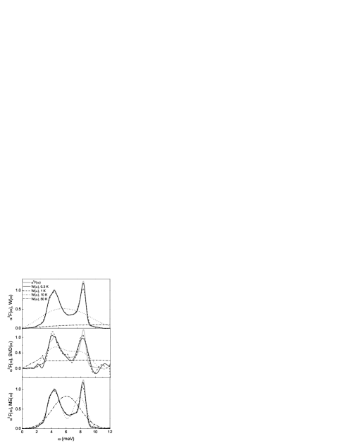
Figure 3: Inversion of finite temperature, normal state $\tau^{-1}_{op}(\omega)$ data computer generated using kernel (11). The solid lines correspond to the temperature $T=0.3\,$K, dashed lines to $1\,$K, dotted lines to $10\,$K, and dash-dotted lines to $50\,$K. The gray solid line represents the $\alpha^{2}F(\omega)$ spectral function applied to calculate the optical scattering rate data. Top frame: Second derivative method. Center frame: SVD method. Bottom frame: MaxEnt method.

Fig. 3 presents the spectra $W(\omega)$, SVD($\omega$), and ME($\omega$) which result from the application of the first two methods of inversion discussed in Sec. II.1. As input we used the finite temperature normal state optical scattering rate for lead generated using kernel (11) (dashed lines of Fig. 2). The top frame presents as a result of the second derivative method, the function $W(\omega)$ as defined in Eq. (6). At the lowest temperature, $T=0.3\,$K the input $\alpha^{2}F(\omega)$ (grey solid line) is perfectly reproduced (solid line), while at $T=1\,$K (dashed line) the high energy peak is already underestimated. At $T=10\,$K (dotted line) the method is no longer able to resolve the two peak structure, and at $T=50\,$K (dash-dotted line) the method fails completely. Nevertheless, it has to be emphasized that no smoothing had to be applied to the input data as no artificial noise was added.

The center frame of Fig. 3 presents the results SVD($\omega$) of a singular value decomposition of Eq. (9) using kernel (11). The svs threshold was set to $10^{-3}$. At $T=0.3\,$K and $1\,$K we obtain reasonable agreement with the $\alpha^{2}F(\omega)$. For energies $>9\,$meV the inversion shows oscillations and SVD($\omega$) even becomes negative which is unphysical. We also see oscillations at low energies and between the two peaks. At $T=10\,$K the SVD method still resolves a hint of a two peak structure in contrast to the second derivative method. Finally, at $T=50\,$K the method fails.

The bottom frame of Fig. 3 presents the results ME($\omega$) of the MaxEnt deconvolution of Eq. (8). Uncorrelated Gaussian noise of $\sigma=10^{-3}$ was added to the computer generated data. For the inversion optimized preblur (see Appendix A) was applied with $b=0.4$ for $T=0.3\,$K, $b=0.46$ for $1\,$K, $b=0.89$ for $T=10\,$K, and $b=1.91$ for $T=50\,$K. The default model was set to $m_{j}=0.01$. The $T=0.3\,$K inversion (solid line) gives almost perfect agreement with the model $\alpha^{2}F(\omega)$ spectral function. At $T=1\,$K the high energy peak is underestimated but reproduced at the appropriate energy. At $T=10\,$K, the two peak structure is still well resolved, only the second peak is underestimated and shifted to lower energies. The result is certainly much better than that of the other two methods. Finally, at $T=50\,$K MaxEnt is no longer able to resolve the two peak structure. Nevertheless, it is quite interesting to note that the area under the dash-dotted curve is $3.95\,$meV which is very close to the area $4.03\,$meV under the original $\alpha^{2}F(\omega)$ spectral function.

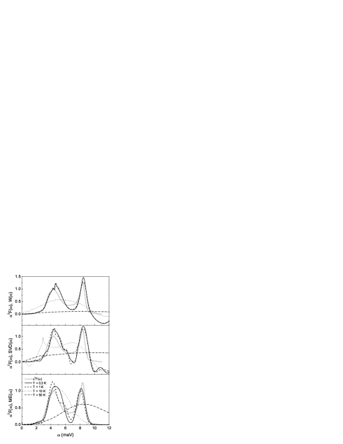
Figure 4: The same as Fig. 3 but now the Eliashberg theory generated normal state, finite temperature $\tau^{-1}_{op}(\omega)$ data (solid lines in Fig. 2) are used as input.

Fig. 2 demonstrated that $\tau^{-1}_{op}(\omega)$ data computer generated from full normal state Eliashberg theory differ from the approximate results of kernel (11). It can also be assumed that metals will more likely follow the predictions of full Eliashberg theory rather than approximate model formulas. It is therefore interesting to investigate how the inversion on the basis of the approximate kernel (11) performs when $\tau^{-1}_{op}(\omega)$ data computer generated within full Eliashberg theory are used for inversion. The result is presented in Fig. 4 which is organized the same way as Fig. 3. The top frame demonstrates the application of the second derivative formula which shouldn’t have any problems because this method is not based on approximate models formulas. Nevertheless, $W(\omega)$ is only in reasonable agreement with the original $\alpha^{2}F(\omega)$ at low temperatures. The low energy peak is over estimated and shifted towards higher energies, the valley between the peaks is too low, the second peak is positioned at the correct energy but its height is over/underestimated. At $T=10\,$K the two peak structure is no longer resolved and at $T=50\,$K the inversion fails. The central frame of Fig. 4 presents the function SVD($\omega$) as a result of an SVD inversion. The svs threshold was set at $10^{-2}$. At low temperatures, the peak positions are at the proper energies, nevertheless the low energy peak is overestimated, the valley between the peaks underestimated, and the high energy peak is too wide. At $T=10\,$K a two peak structure is resolved but both peaks are placed at the wrong energies. At $T=50\,$K the method fails altogether. It is typical for this method to show oscillations at energies $>9\,$meV which result in unphysical negative contributions even at energies below $\omega_{D}$.

Before applying the MaxEnt inversion uncorrelated Gaussian noise of $\sigma=0.1$ was added to the input data. For the temperature $0.3\,$K and $1\,$K the preblur parameter was optimized to 0.54 at higher temperatures no preblur was applied. The default model was set to $0.01$. At low temperatures MaxEnt overestimates the low energy peak and/or makes it broader. The valley between the peaks is too low, the second peak is resolved reasonably well and is at the proper position but underestimated in height. At higher temperatures the two peak structure is no longer resolved ($T=10\,$K, dotted line and $T=50\,$K, dash-dotted line). Nevertheless, data reconstruction is within error bars and this proves that we face in this case a deconvolution problem which is particularly ill conditioned.

All this demonstrates quite clearly that the application of methods of inversion based on approximate models to experimental data (represented here by computer generated $\tau^{-1}_{op}(\omega)$ data using full Eliashberg theory) can quite easily result in deconvoluted spectra $\alpha^{2}F(\omega)$ which will be close but not necessarily equal to the real electron-phonon spectrum which governs the interaction. In particular, the deviations from the gray solid lines in the central and bottom frame of Fig. 4 represent the deviations from the ‘real’ $\alpha^{2}F(\omega)$ which are required by the approximate kernels to reproduce the input optical scattering rate data as well as possible.

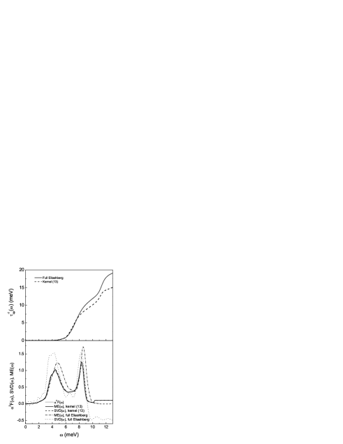
Figure 5: Top frame: The computer generated superconducting state optical scattering rate $\tau^{-1}_{op}(\omega)$ for Pb at $T=0.05T_{c}$ with $T_{c}=7.2K$. The solid line is based on the full Eqs. (20) while the dashed line is obtained using the simplified kernel (13). Bottom frame: The gray solid line symbolizes the $\alpha^{2}F(\omega)$ of Pb. The solid line is the result of the inversion of $\tau_{op}^{-1}(\omega)$ data computer generated using kernel (13) (dashed line in the top frame of this figure) using the MaxEnt method while the dashed line corresponds to an SVD inversion. The dash-dotted and dotted lines present equivalent results but now for full Eliashberg data (solid line in the top frame of this figure).

We now move on to a discussion of superconducting state data. The top frame of Fig. 5 presents the results for the superconducting state optical scattering rate $\tau^{-1}_{op}(\omega)$ in Pb at $T=0.05T_{c}$ with $T_{c}=7.2\,$K. The solid line was obtained on evaluation of the full Eqs. (20) and (21) taken for $s$-wave symmetry of the superconducting order parameter and a Coulomb pseudopotential $\mu^{\ast}=0.1438$. The dashed line is for comparison and was obtained from kernel (13) using the electron-phonon spectral density $\alpha^{2}F(\omega)$ shown by a gray solid line in the bottom frame of this figure. The approximate kernel (13) is evaluated with $\Delta_{0}=1.39\,$meV, the gap edge predicted by the full Eliashberg calculation.

The bottom frame of Fig. 5 presents the result of SVD as well as MaxEnt inversions based on the approximate kernel (13). The dashed line corresponds to the SVD inversion (svs threshold was set at $10^{-2}$) of the optical scattering rate generated using kernel (13) (dashed line in the top frame of Fig. 5) and $\Delta_{0}=1.39\,$meV. As expected, the agreement is almost perfect. The dotted line, on the other hand, shows the result of an SVD inversion of full Eliashberg data (solid line in the top frame). Here, the lower, transverse peak centered around $\sim 4\,$meV is broader and the area under the peak is larger. The same holds for the upper, longitudinal phonon peak but the differences are now less pronounced. Beyond $\sim 9\,$meV the dotted line becomes negative giving unphysical results. These differences are due to the use of the approximate kernel (13) in the inversion process.

The MaxEnt inversion was performed by attaching error bars of $\sigma=10^{-2}$ to the data and by adding uncorrelated Gaussian noise of the same $\sigma$. Furthermore, no preblur was applied and the default model was set to 0.1. The solid line is the MaxEnt inversion of the data computer generated with the help of kernel (13) (dashed line in the top frame of Fig. 5). Again we achieve perfect agreement. At energies $>10.5\,$meV the function ME($\omega$) levels off at the value 0.1 demonstrating the influence of the chosen default model. The dash-dotted curve, on the other hand, is based on full Eliashberg theory generated input data (solid line in the top frame of this figure). Both peaks are now overestimated in their height and width and are shifted towards higher energies. Nevertheless, ME($\omega$) never becomes negative which proves that there exists a positive definite solution for the deconvolution problem of Eq. (7). As experimental data are more likely to be close to full Eliashberg theory results, the deconvolution of Eq. (7) on the basis of kernel (13) will result in an electron-phonon spectral density $\alpha^{2}F(\omega)$ which will not agree in all details with the real spectral density despite the fact that the input data will be excellently reproduced. The only possible check for the validity of the deconvoluted electron-phonon spectral density SVD($\omega$) or ME($\omega$) is using it to calculate the optical scattering rate based on full Eliashberg theory and compare with the data. Such a comparison will then result in necessary readjustments of the deconvoluted spectrum.

III.2 High-$Tc$ cuprates

In contrast to the normal metal lead, the high $T_{c}$ cuprates are not likely to be electron-phonon systems, they are known to be highly correlated systems. There is a class of models used to describe such systems which we will refer to as boson exchange models. They have many common elements with the electron-phonon case. In particular, there exists a well developed literature on the Nearly Antiferromagnetic Fermi Liquid model (NAFFL) introduced by Pines and collaborators.pines1 ; pines2 The exchange bosons are antiferromagnetic spin fluctuations as described by Millis et al.mmp (MMP). Within this model the Eliashberg equations are retained in a zeroth order approximation neglecting possible vertex corrections which go beyond Migdal’s theorem. The electron-phonon spectral density $\alpha^{2}F(\omega)$ is replaced by the imaginary part of the spin susceptibility multiplied by the square of a coupling of the spin fluctuations to the charge carriers. In general, this interaction is anisotropic and not pinned to the Fermi surface.branch Nevertheless, as a first approximation, one can work with a simple interaction spectral function $I^{2}\chi(\omega)$ which replaces the $\alpha^{2}F(\omega)$ of Eliashberg theory. Carbotte et al.carb3 found that in optimally doped, twinned YBCO single crystals the measured normal state optical scattering rate $\tau^{-1}_{ex}(\omega)$, reported by Basov et al.bas1 , can be well described by a single MMP form:

$$I^{2}\chi(\omega)=I^{2}\frac{\omega/\omega_{SF}}{1+(\omega/\omega_{SF})^{2}}.$$ (15)

The two parameters, the square of the coupling constant $I$ and the characteristic spin fluctuation energy $\omega_{SF}$ were determined from a least squares fit to the data in the energy interval $0\leq\omega\leq 250\,$meV. The values $I^{2}=0.83$ and $\omega_{SF}=20\,$meV have been reported by CSB.

Based on the results for lead we cannot necessarily expect inversions of $\tau^{-1}_{op}(\omega)$ measured around $T=100\,$K or even higher will be feasible. To investigate this, normal state $\tau^{-1}_{op}(\omega)$ data are computer generated at various temperatures, namely $T=1\,$K, $10\,$K, $50\,$K, and $100\,$K using either kernel (11) or full Eliashberg theory with an $I^{2}\chi(\omega)$ determined by Eq. (15) and with the above values for the parameters $I^{2}$ and $\omega_{SF}$. The results of the inversion based on the approximate kernel (11) are discussed in Fig. 6 with $\tau^{-1}_{op}(\omega)$ data generated using kernel (11) and, in Fig. 7 with $\tau^{-1}_{op}(\omega)$ generated by full Eliashberg theory.

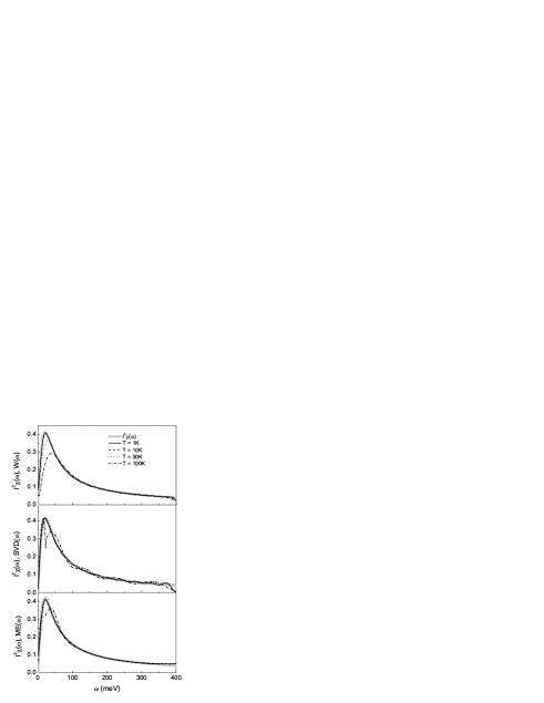
Figure 6: The same as Fig. 3 with the $\alpha^{2}F(\omega)$ replaced by the $I^{2}\chi(\omega)$ defined by Eq. (15) with $I^{2}=0.83$ and $\omega_{SF}=20\,$meV. The solid lines corresponds to $T=1\,$K, the dashed lines to $10\,$K, the dotted lines to $50\,$K, and the dash-dotted lines to $100\,$K.

The top frame of Fig. 6 presents results for $W(\omega)$ from the second derivative method. At the two lowest temperatures, namely $T=1\,$K (solid line) and $10\,$K (dashed line) the $I^{2}\chi(\omega)$ spectrum (gray solid line) is almost perfectly reproduced. At higher temperatures, namely at $T=50\,$K (dotted line) and $100\,$K (dash-dotted line) the inverted spectrum develops a less pronounced peak which is also shifted towards higher energies. In the tail ($\omega>100\,$meV) noise develops in the inverted spectrum. Nevertheless, in contrast to lead with its narrow two peak structure the simple MMP form can easily be inverted from optical scattering rate data even at temperatures around $100\,$K.

The center frame of Fig. 6 presents the results SVD($\omega$) of a singular value decomposition. The svs threshold was set at $10^{-3}$ for $T=1\,$K and $10\,$K and was increased to $10^{-2}$ for $T=50\,$K and $100\,$K. The inverted spectrum agrees reasonably well with the original spectrum at low energies, $\omega<75\,$meV. At higher energies significant oscillations occur. We also note for $T=100\,$K a typical splitting of the peak at $20\,$meV into two peaks. This is an indication of a particularly ill conditioned inversion problem. This phenomenon can be observed for rather narrow and fast rising peaks.sivia

The bottom frame of Fig. 6 presents the results ME($\omega$) of a MaxEnt deconvolution. The error bars on the data were determined by $\sigma=0.15$ and uncorrelated Gaussian noise of the same $\sigma$ was added. No preblur was applied. The default model was set to 0.05. This ensures that the spectrum ME($\omega$) agrees at high energies with $I^{2}\chi(\omega)$. The agreement with the original $I^{2}\chi(\omega)$ spectral function (gray solid line) is excellent up to temperatures of $50\,$K. At $100\,$K the peak at $20\,$meV is not as well resolved and shows tendency towards a splitted peak similar to the SVD inversion at the same temperature. Otherwise, the agreement is still rather good.

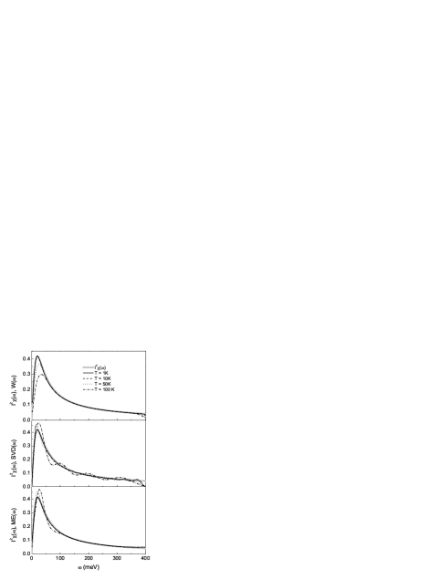
Figure 7: The same as Fig. 6 but now Eliashberg theory generated optical scattering rates have been used as input for the inversion.

The results presented in Fig. 7 are very similar to the ones shown in Fig. 6 with the difference that SVD and MaxEnt (error bars were determined by $\sigma=0.2$, uncorrelated Gaussian noise of the same $\sigma$ was added, no preblur) now overestimate the peak at $20\,$meV. The SVD result for $100\,$K (dash-dotted line in the center frame of Fig. 7) develops a slight tendency for a splitted peak at $20\,$meV. All this is the result of the minor differences between the optical scattering rates calculated from kernel (11) and full Eliashberg theory and the top frame of Fig. 8 demonstrates how little these differences are.

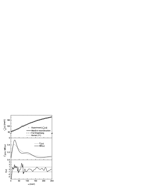
Figure 8: Top frame: Experimental normal state optical scattering rate $\tau^{-1}_{ex}(\omega)$ at $T=95\,$K for an optimally doped, twinned YBCO_6.95 single crystal as reported by Basov et al.bas1 (solid gray diamonds). The black solid line corresponds to the MaxEnt reconstruction based on kernel (11) using the spectral function ME($\omega$) shown in the middle frame of this figure (black solid line). The dashed line presents $\tau^{-1}_{op}(\omega)$ of a full Eliashberg calculation based on the spectral function $I^{2}\chi(\omega)$ shown by a gray solid line in the middle frame of this figure and the dotted line corresponds to $\tau^{-1}_{op}(\omega)$ computer generated using kernel (11) and the same $I^{2}\chi(\omega)$. Bottom frame: The residual $r(\omega)$ according to Eq. (14) of the MaxEnt data reconstruction.

We proceed to a study of the MaxEnt inversion of experimental data and make use of the $T=95\,$K normal state optical scattering rate measured by Basov et al.bas1 on an optimally doped, twinned YBCO_6.95 single crystal. Fig. 8 presents the result of a MaxEnt inversion. We assume the experimental data $\tau^{-1}_{ex}(\omega)$ to be contaminated by a substantial uncorrelated Gaussian noise of $\sigma=2.5$. The inversion is performed on the basis of kernel (11) and the resulting spectral function ME($\omega$) is shown as a solid line in the middle frame of Fig. 8. ME($\omega$) then replaces $\alpha^{2}F(\omega)$ in Eq. (7) which is used to calculate the reconstructed optical scattering rate shown by a solid line in the top frame of Fig. 8. It reproduces excellently the experimental data (gray solid diamonds). For comparison, the top frame of this figure contains two more results, namely $\tau^{-1}_{op}(\omega)$ calculated from full Eliashberg theory (dashed line) using the $I^{2}\chi(\omega)$ reported by CSB, namely $I^{2}=0.83$ and $\omega_{SF}=20\,$meV (gray solid line in the center frame of Fig. 8). The dotted line, on the other hand, corresponds to $\tau^{-1}_{op}(\omega)$ calculated from Eq. (7) using kernel (11) and the same $I^{2}\chi(\omega)$. Obviously, the two results are very close with the dotted line slightly above the dashed one at low energies. The opposite holds for high energies. This is in agreement with the result found for lead (see Fig. 2).

Finally, the bottom frame of Fig. 8 shows the residual $r(\omega)$ which is a measure for the quality of the data reconstruction. Apart from the low energy region the reconstruction is within the assumed standard deviation (indicated by the two straight lines at 1 and -1) of $\sigma=2.5$. The result is to be compared with the $r(\omega)$ shown in the bottom frame of Fig. 1 which results from the reconstruction of computer generated data with additional uncorrelated Gaussian noise. The $r(\omega)$ in the bottom frame of Fig. 8 is a rather smooth function which contains for energies $>70\,$meV very little stochastic elements which could be identified as noise. The various data points appear to be rather correlated an effect which could either be attributed to an additional background function $B(\omega)$ [see Eq. (2)] or to a ‘real’ signal. Nevertheless, what is important here is the fact that the inverted ME($\omega$) has a nonzero contribution even at energies $>150\,$meV thus establishing a high energy background in $I^{2}\chi(\omega)$ as predicted by CSB. Finally, as both spectral functions presented in the central frame of Fig. 8 reconstruct the experimental data (solid gray diamonds in the top frame of Fig. 8) equally well, they can be used as valid spectral functions because of the non-uniqueness of the deconvolution problem. Further calculations and comparison with other experiments than optical conductivity may then help to discriminate between these two spectra. It is interesting to point out that the area under $I^{2}\chi(\omega)$ ($42\,$meV) is approximately reproduced by the area under the spectrum ME($\omega$) ($41.4\,$meV) which could be used to explain the oscillations in ME($\omega$) as a result of the enhanced main peak at $20\,$meV.

Tu et al.tu measured the optical scattering rate of optimally doped Bi₂Sr₂CaCu₂O_8+δ (Bi2212) single crystals at various temperatures. They derived, using data analysis different from the methods discussed here, that even in the normal state at $100\,$K a resonance peak is seen in the function $W(\omega)$ while it is rather featureless at $295\,$K. Schachinger and Carbotteschach1 also analyzed these data using a combination of the second derivative method and least squares fits to the data. In particular, they found that the $T=295\,$K data are well described by an MMP form (15) in the energy region $0\leq\omega\leq 250\,$meV. The least squares fit determined the parameters $I^{2}=0.655$ and $\omega_{SF}=82\,$meV using full Eliashberg theory in the fitting procedure.

As MaxEnt turned out to be a rather powerful inversion technique we revisit the Bi2212 data analysis. We assume the experimental data of Tu et al. to contain uncorrelated Gaussian noise of $\sigma=2.0$ for $T=100\,$K and $\sigma=3.0$ for $T=200\,$K and $295\,$K. The preblur parameter was set to 5 for $T=100\,$K and to 10 for the other two temperatures. The default model was set to 0.1. The inversion is based on the application of the approximate kernel (11). Fig. 9 discusses the results of

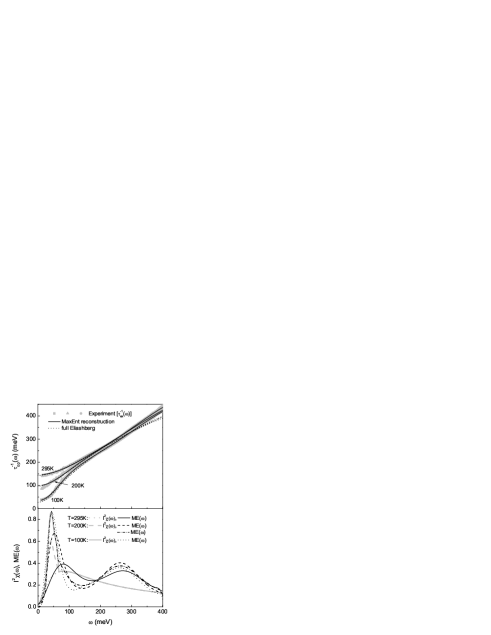
Figure 9: Top frame: Experimental optical scattering rate datatu $\tau^{-1}_{ex}(\omega)$ of Bi2212 (gray solid symbols) reconstructed using the MaxEnt method (black solid line) for various temperatures, namely $T=100\,$K, $200\,$K, and $295\,$K. The dotted lines correspond to data generated by full Eliashberg theory using the $I^{2}\chi(\omega)$ spectra reported by Schachinger and Carbotte.schach1 Bottom frame: The spectral function ME($\omega$) (black solid line for $295\,$K, black dashed, black dash-dotted for $200\,$K, and black dotted for $100\,$K) as a result of the MaxEnt inversion of the experimental data (gray solid symbols in the top frame of this figure). The gray lines (solid for $295\,$K, dotted for $200\,$K, and dashed for $100\,$K) show the $I^{2}\chi(\omega)$ spectra reported by Schachinger and Carbotte.schach1 The black dash-dotted line presents results of a MaxEnt inversion of the $200\,$K data (solid gray triangles in the top frame) using the $I^{2}\chi(\omega)$ (gray dotted line) as the default model.

our calculations. The top frame presents the data reconstruction and the bottom frame the inverted spectral function ME($\omega$) in comparison to $I^{2}\chi(\omega)$ spectral functions suggested by Schachinger and Carbotte.schach1 It is quite clear that the data reconstruction (black solid lines in the top frame of Fig. 9) is in excellent agreement with the original data (gray solid symbols) at all temperatures. The black dotted lines correspond to $\tau^{-1}_{op}(\omega)$ data generated from full Eliashberg theory using the $I^{2}\chi(\omega)$ spectral functions presented in the bottom frame of Fig. 9 by gray lines, namely solid for $100\,$K, dashed for $200\,$K, and dotted for $295\,$K. The full Eliashberg results follow the data rather nicely in the energy range $0\leq\omega\leq 250\,$meV and then deviate systematically to smaller values for energies $>250\,$meV. Thus, the MMP form alone is not sufficient to explain the energy dependence of $\tau^{-1}_{ex}(\omega)$ in the whole energy range $0\leq\omega\leq 400\,$meV.

Comparing the spectral functions ME($\omega$) to the $I^{2}\chi(\omega)$ spectra demonstrates rather good agreement at low energies for $T=100\,$K (black dotted line, gray solid line). Both spectra show a pronounced peak at $43\,$meV and they even agree in height and width of the peak which is rather fortuitous. At $T=200\,$K (black dashed line, gray dashed line) both spectra develop a less pronounced peak with the peak in ME($\omega$) shifted away from $43\,$meV to higher energies. Such a shift towards higher energies with increasing temperatures has already been observed in the analysis of computer generated $\tau^{-1}_{op}(\omega)$ data for YBCO_6.95, Fig. 6, and this peak in the ME$(\omega$) could very well correspond to a $43\,$meV peak in the ‘real’ spectrum. Finally, at $T=295\,$K (black solid line, gray dotted line) both spectra agree in showing a rather flat MMP like structure peaked around $82\,$meV with no indication of a resonance peak. This analysis corroborates the results reported by Tu et al.tu and by Schachinger and Carbotte.schach1

It is quite important to notice that all ME($\omega$) spectra develop a second structure of comparable height around $\sim 260\,$meV for all temperatures. Such a structure is missing in the $I^{2}\chi(\omega)$ spectra. This additional structure is required for a faithful reconstruction of the experimental $\tau^{-1}_{ex}(\omega)$ data at higher energies. To include one more check we repeated the inversion of the $T=200\,$K $\tau_{ex}^{-1}(\omega)$ data using MaxEnt but now without preblur and with the default model set to the $I^{2}\chi(\omega)$ spectrum for $200\,$K (gray dashed line in the bottom frame of Fig. 9). The result is presented by the black dash-dotted line in the bottom frame of Fig. 9. In this case the optical resonance can be found at $43\,$meV in contrast to the calculation with the constant default model (black dashed line) but it is now significantly enhanced.

Figure 10: The residual $r(\omega)$ of the data reconstruction presented in the top frame of Fig. 9. The top frame is for $T=100\,$K, the middle frame for $200\,$K, and the bottom frame for $295\,$K.

Even the kink in the $I^{2}\chi(\omega)$ spectrum at about $60\,$meV is reproduced in ME($\omega$). What is important, though, is the fact that the additional high energy structure around $260\,$meV appears again with approximately the same strength as in all other results. Thus, it seems to be a real and new feature not captured by a simple MMP form and this proves that the charge carrier-exchange boson spectral function $I^{2}\chi(\omega)$ in the cuprates has non-zero contributions up to at least $400\,$meV, a property which cannot be explained by a pure phonon mechanism.

It is interesting to note in closing that, for instance, ME($\omega$) for $T=295\,$K can be described using a simple model, namely the original MMP form which is replaced for $\omega>170\,$meV by a second MMP form peaked at $\omega_{SF}=260\,$meV. A least squares fit to $\tau^{-1}_{ex}(\omega,T=295\,$K) using full Eliashberg theory provides an $I^{2}=0.55$ for this second MMP form and agreement with the data is achieved over the whole energy range $0\leq\omega\leq 400\,$meV. This is a second, independent proof of the existence of this additional high energy structure in $I^{2}\chi(\omega)$ for optimally doped Bi2212.

In Fig. 10 the residual $r(\omega)$ of our analysis of the Bi2212 data is presented. The top frame is for $100\,$K, the middle frame for $200\,$K, and the bottom frame for $295\,$K. The residual clearly shows a stochastic component which is much smaller than the assumed values for $\sigma$ in the energy region $100\leq\omega\leq 350\,$meV. It can be identified as a noise contribution. There is obviously, another slowly oscillating contribution to $r(\omega)$ which is almost identical in its frequency dependence at $100\,$ and $200\,$K but it doubles its period at $295\,$K. This contribution is very likely to be a background signal $B(\omega)$ generated by the experimental equipment.

We proceed to investigate the inversion of superconducting state $\tau^{-1}_{op}(\omega)$ data for YBCO_6.95. We use for computer generated $\tau^{-1}_{op}(\omega)$ data the spectral function $I^{2}\chi(\omega)$ reported by CSB for $T=10\,$K. It was derived from experimental superconducting state $\tau^{-1}_{op}(\omega)$ data reported by Basov et al.bas1 at $T=10\,$K for an optimally doped, twinned YBCO_6.95 single crystal. This $I^{2}\chi(\omega)$ is based on the normal state $I^{2}\chi(\omega)$ for YBCO_6.95 which is an MMP form (15) with $I^{2}=0.83$ and $\omega_{SF}=20\,$meV (gray squares in Figs. 6 and 7). Superimposed is a pronounced peak at $\omega=41\,$meV which was found by applying the second order derivative method to the experimental data. The final form, shown using gray solid squares in the middle and bottom frame of Fig. 11, was established by a fit of full Eliashberg $\tau^{-1}_{op}(\omega)$ results to experiment.

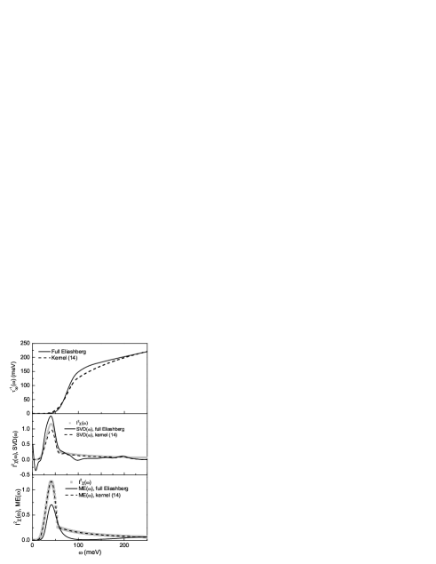
Figure 11: Top frame: The computer generated superconducting state optical scattering rate $\tau^{-1}_{op}(\omega)$ at $T=10\,$K calculated from full Eliashberg theory (solid line) or from kernel (14) (dashed line) using the $I^{2}\chi(\omega)$ spectrum shown as the gray solid lines in the middle and bottom frame of this figure. Middle frame: The gray solid line corresponds to the spectral function $I^{2}\chi(\omega)$ reported by CSB for superconducting YBCO_6.95 at $T=10\,$K. The solid line shows the spectral function SVD($\omega$) as a result of an SVD inversion of the full Eliashberg result (solid line in the top frame of this figure). The dashed line shows the same but now the scattering rate generated by kernel (14) is used as input. Bottom frame: The same as the middle frame. ME($\omega$) is the result of a MaxEnt inversion.

This spectrum which extends to $400\,$meV was applied by Schachinger et al.schach7 within full Eliashberg formalism. The authors demonstrated that it was possible to reproduce numerous superconducting state properties of optimally doped YBCO_6.95 in their temperature and energy dependence within experimental errors. The need for $I^{2}\chi(\omega)$ to extend to several hundred meV has also been reviewed by Basov and Timusk.bas5

The top frame of Fig. 11 presents computer generated superconducting state $\tau^{-1}_{op}(\omega)$ data at $T=10\,$K as a function of energy. The solid line gives the result of a full Eliashberg calculation using the solutions of Eqs. (20) and (21) on the basis of the spectral function $I^{2}\chi(\omega)$ just described. Eliashberg theory also provides a value for the zero temperature gap amplitude $\Delta_{0}=22.03\,$meV. The dashed line presents the optical scattering rate as calculated using kernel (14), the above value for $\Delta_{0}$, and the same spectral function $I^{2}\chi(\omega)$. The two results differ substantially in the energy region $70\leq\omega\leq 200\,$meV.

The results of an SVD inversion are shown in the middle frame of Fig. 11. The solid line presents the spectral function SVD($\omega$) found from inverting the full Eliashberg results (solid line in the top frame of this figure) on the basis of kernel (14) using $\Delta_{0}=22.03\,$meV as an external parameter. The dashed line corresponds to the inversion of the scattering rate generated by kernel (14) using the same value for $\Delta_{0}$ (dashed line in the top frame of this figure). In both cases the svs threshold was set to $10^{-2}$. The agreement of both spectra SVD($\omega$) with the original $I^{2}\chi(\omega)$ (gray solid line) is rather poor keeping in mind that the inversion is based on computer generated data.

The bottom frame of Fig. 11 is organized as the middle frame of this figure. It presents spectra ME($\omega$) as a result of a MaxEnt inversion. For the inversion of $\tau^{-1}_{op}(\omega)$ represented by the dashed line in the top frame of this figure an error bar of $\sigma=0.01$ was assumed and no noise was added to the data. The inversion was performed using historical MaxEnt with $\gamma^{2}=N_{1}$ as convergence criterion. The resulting spectral function ME($\omega$) is represented by a dashed line. The agreement with the spectrum $I^{2}\chi(\omega)$ (solid gray line) employed to generate $\tau^{-1}_{op}(\omega)$ is perfect as was to be expected. The inversion of full Eliashberg theory generated $\tau^{-1}_{op}(\omega)$ data (solid line in the top frame of this figure) based on the same $I^{2}\chi(\omega)$ is less successful as the resulting spectrum ME($\omega$) (solid line) demonstrates. For the inversion an error of $\sigma=0.7$ was attached to the $\tau^{-1}_{op}(\omega)$ data but we did not add noise. Furthermore, $\Delta_{0}$ had to be reduced to $21\,$meV in order to keep the peak in ME($\omega$) at $41\,$meV. The peak height is now grossly underestimated and the spectrum ME($\omega$) does no longer reproduce the normal state background spectrum. Such a result was expected because of the pronounced differences particularly in this energy region between the full Eliashberg theory generated data and the data generated using kernel (14).

We proceed and study the application of the MaxEnt inversion based on kernel (14) using experimental superconducting state $\tau^{-1}_{op}(\omega)$ data. The top frame of

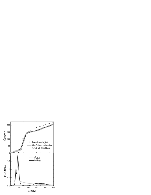
Figure 12: Top frame: The superconducting state optical scattering rate $\tau^{-1}_{ex}(\omega)$ at $T=10\,$K for an optimally doped, twinned YBCO_6.95 single crystal. The solid gray diamonds present the original data by Basov et al.bas1 . The solid line shows the MaxEnt reconstruction of the input data while the dashed line shows the result of a full Eliashberg theory calculation based on the spectrum $I^{2}\chi(\omega)$ reported by CSB for $T=10\,$K. Bottom frame: The gray solid line presents the $I^{2}\chi(\omega)$ spectrum suggested by CSB for superconducting YBCO_6.95 at $T=10\,$K. The solid line shows the spectrum ME($\omega$) as a result of the inversion of the experimental data by Basov et al.bas1 represented by solid gray diamonds in the top frame of this figure.

of Fig. 12 presents the original data by Basov et al.bas1 reported for an optimally doped, twinned YBCO_6.95 single crystal at $T=10\,$K (solid gray diamonds). The inversion of this data is performed using historical MaxEnt based on kernel (14) with $\gamma^{2}=N_{1}$ as criterion of convergence. An error bar of $\sigma=3.5$ was attached to the data and the default model was set to 0.05. The resulting spectrum ME($\omega)$ is presented as black solid line in the bottom frame of Fig. 12. This spectrum was found using $\Delta_{0}=21\,$meV. This allowed to place the main peak in ME($\omega$) at $41\,$meV. It is obvious that the inverted spectrum ME($\omega$) differs substantially from the $I^{2}\chi(\omega)$ spectrum (gray solid line) reported by CSB. It shows peak splitting of the resonance peak at $41\,$meV and the low energy peak ($\omega<5\,$meV) in ME($\omega$) is caused by an attempt to use MaxEnt to extrapolate to very small energies which are not supported by the $\tau^{-1}_{ex}(\omega)$ data. Nevertheless, the data reconstruction (black solid line in the upper frame of Fig. 12) is excellent. We added for comparison (dashed line in the upper frame of Fig. 12) the optical scattering rate as generated by full Eliashberg theory using $I^{2}\chi(\omega)$. The agreement with the data does not seem to be good enough to justify the particular shape of $I^{2}\chi(\omega)$ discussed above. Nevertheless, one has to keep in mind that all calculations presented here are performed without including impurities, i.e.: in the pure case limit. Adding impurities improves the agreement between full Eliashberg theory and experiment substantially.schach1

As a last example we present the reconstruction of experimental superconducting state $\tau^{-1}_{ex}(\omega)$ data reported by Tu et al.tu for an optimally doped Bi2212 single crystal at $T=6\,$K.

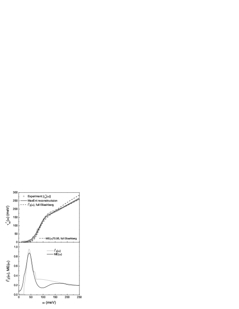
Figure 13: The same as Fig. 12 but now for a superconducting optimally doped Bi2212 single crystal at $T=6\,$K. The data have been reported by Tu et al.tu The additional dash-dotted line in the top frame describes the result of a full Eliashberg calculation based on the ME($\omega$) spectrum which was down scaled by a factor 0.95.

The results are presented in Fig. 13 which is organized the same way as Fig. 12. For the MaxEnt data reconstruction an error bar determined by $\sigma=3.0$ was attached to the data. Historical MaxEnt with $\gamma^{2}=N_{1}$ as criterion for convergence was applied. The default model was set to 0.2. The inversion is based on kernel (14) and the spectrum $I^{2}\chi(\omega)$ reported by Schachinger and Carbotteschach1 for $T=6\,$K is shown as a gray solid line in the bottom frame of Fig. 13 for comparison. It contains a peak at $43\,$meV and an MMP form (15) as background with $I^{2}=0.655$ and $\omega_{SF}=82\,$meV. In this case the agreement between the inverted spectrum ME($\omega$) (solid line in the bottom frame of Fig. 13) and $I^{2}\chi(\omega)$ is much better in comparison to YBCO_6.95. This confirms the analysis of Schachinger and Carbotteschach1 as well as a previous analysis of Bi2212 data by Schachinger and Carbotteschach2 based on data published by Puchkov et al.puchkov We added one more result to the top frame of Fig. 13 presented by a dash-dotted line. It corresponds to the result of a full Eliashberg calculation based on the ME($\omega$) spectrum (down scaled by a factor of 0.95) instead of $I^{2}\chi(\omega)$. The agreement with experiment is now very good. In particular, the ‘overshoot’ right after the main rise in the optical scattering ratebas5 is better resolved than in the original Eliashberg calculation (dashed line). Thus, the existence of this overshoot is an indication that a dip exists in the $I^{2}\chi(\omega)$ spectrum immediately following the resonance peak. This dip will, of course, not be as pronounced as it appears in ME($\omega$) because the major part of it stems from the differences between the approximate kernel (14) and full Eliashberg theory. If the ME($\omega$) spectrum is, furthermore, employed to calculate the zero temperature gap amplitude $\Delta_{0}$ within full Eliashberg theory a value of $32\,$meV is found, in excellent agreement with experimental results.zas1 ; zas2 We also note that the optical scattering rate $\tau^{-1}_{ex}(\omega)$ in the top frame of Fig. 12 (gray solid diamonds) develops a moderate overshoot following the main rise around $80\leq\omega\leq 110\,$meV. Thus, also in this case not all of the dip which follows the resonance peak in the ME($\omega$) spectrum can be attributed to the differences in the approximate kernel (14) and full Eliashberg theory.

III.3 The least squares fit method

It has been pointed out in the previous subsection that the least squares fit method has already been applied rather successfully to invert $I^{2}\chi(\omega)$ spectra from experiment using full Eliashberg theory together with additional information gathered by other means. This method is rather clumsy to handle and time

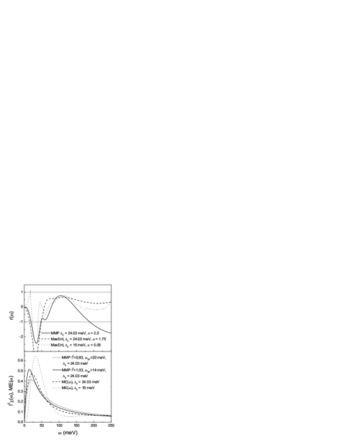
Figure 14: Top frame: The residual $r(\omega)$. The solid line corresponds to a least square fit of an MMP form to computer generated optical scattering rate data generated by full Eliashberg theory, $\Delta_{0}=24.03\,$meV and $\sigma=2.0$ was assumed. The dashed line corresponds to a MaxEnt analysis of the same data for $\sigma=1.75$ keeping $\Delta_{0}$ fixed and the dotted line is for $\sigma=0.05$ and $\Delta_{0}=15\,$meV. The main part of the various $r(\omega)$ curves is within $\pm 1$ indicating perfect data reconstruction within the assumed error. Bottom frame: The spectrum $I^{2}\chi(\omega)$ (gray solid line) is the input spectrum for the full Eliashberg calculation. The solid line gives the inverted spectrum as a result of a least squares fit to the data, the dashed line the result of a MaxEnt inversion both with $\Delta_{0}=24.03\,$meV. Finally, the dotted line shows the spectrum ME($\omega$) which resulted from an optimal data reproduction using MaxEnt but now $\Delta_{0}=15\,$meV.

consuming as one cannot develop a closed algorithm which allows one to fit parameters directly given some standard deviation $\sigma$ which plays the role of the nuisance parameter. Therefore, we want to study the least squares fit method based on the approximate kernel (14) for the superconducting state of a $d$-wave superconductor. The $\tau^{-1}_{op}(\omega)$ data are generated from full Eliashberg theory for the superconducting state at $T=10\,$K using for $I^{2}\chi(\omega)$ an MMP form (15) with $I^{2}=0.83$ and $\omega_{SF}=20\,$meV (gray solid line in the bottom frame of Fig. 14). The zero temperature gap $\Delta_{0}=24.03\,$meV. The least squares fit method is now applied to determine $I^{2}$ and $\omega_{SF}$ of an MMP form by a least squares fit to $\tau^{-1}_{op}(\omega)$ in the energy region $0\leq\omega\leq 250\,$meV. The error bar attached to the input data is given by $\sigma=2.0$. (This particular value of the standard deviation appears to be a realistic value for the reconstruction of experimental data as was demonstrated in the previous subsection.) No noise was added. A consistent data reconstruction was achieved with the parameters $I^{2}=1.03$ and $\omega_{SF}=14\,$meV. This becomes apparent from Fig. 14 in which the results of the least squares method are illustrated. The solid line in the top frame of this figure shows the residual $r(\omega)$, Eq. (5), which is on average well within the assumed $\sigma$. This insures a correct data reconstruction. The bottom frame of this figure compares the least squares fit spectrum (solid line) to the original $I^{2}\chi(\omega)$ indicated by a gray solid line. It is interesting to compare the areas under these two spectra, they are $41.5\,$meV and $42\,$meV, respectively, a difference of about 1%. The parameter $\lambda$ which is two times the first inverse moment of $I^{2}\chi(\omega)$ is also a good parameter to compare. We get $\lambda=2.48$ and $3.09$, respectively.

Figure. 14 contains additional information. We use the MaxEnt method to generate an ‘educated guess’ for a later least squares fit to data based on full Eliashberg theory. If we use $\Delta_{0}=24.03\,$meV and assume $\sigma=1.75$ historical MaxEnt reproduces the input data almost equally well as our least squares fit. (Dashed line in the top frame of Fig. 14.) The resulting spectrum ME($\omega$) (dashed line in the bottom frame of Fig. 14) has its peak at a slightly higher energy ($\sim 24\,$meV) as compared to the original $I^{2}\chi(\omega)$ but otherwise, the input spectrum is reproduced rather well, albeit not by an MMP form. The area under this spectrum is $40\,$meV and $\lambda=3.22$, again close to the result of the least squares fit ‘inversion’. We also include, for comparison, the result of a MaxEnt deconvolution with the emphasis on optimal data reconstruction. We reduce the error bar on the input data to $\sigma=0.05$ and use $\Delta_{0}$ as a parameter to be adjusted in order to achieve this goal. An almost perfect reproduction is possible if $\Delta_{0}$ is reduced to $15\,$meV. This becomes apparent from the residual $r(\omega)$ shown as a dotted line in the top frame of Fig. 14. The resulting spectrum ME($\omega$) is presented by a dotted line in the bottom frame. The peak is now shifted to much higher energies, it is wider, and is greater in height as compared to the original $I^{2}\chi(\omega)$. The area under the spectrum is $40.2\,$meV and $\lambda=1.92$. This demonstrates clearly the approximate nature of kernel (14) and that a value for $\Delta_{0}$ found from optimum data reproduction is not physically significant. Instead, one has to treat $\Delta_{0}$ as an external parameter to the inversion process which is to be determined by other means like, for instance, scanning tunneling microscopy.zas1 ; zas2

While the various methods of inversion described in this section lead to significant differences in the value of $\lambda$ obtained, the area under the spectral density varies very little. The differences in $\lambda$ can be traced mainly to variations in the position of the main fluctuation peak and, therefore, it is recommended that independent information on the position of this peak be used, for example from neutron scattering.

As a result of this study one can say that given additional information, like the value of the zero temperature gap amplitude, both methods, least squares fit and MaxEnt, result in comparable spectra, nevertheless, they differ qualitatively and quantitatively from the ‘real’ spectrum $I^{2}\chi(\omega)$. This emphasizes the role of additional information beyond the optical data for a successful data analysis.

IV Conclusion

There exists a well established formalism that relates the electron-phonon spectral density $\alpha^{2}F(\omega)$ to the infrared conductivity. It applies to the superconducting as well as normal state and involves the Eliashberg equations plus a Kubo formula which gives the optical conductivity $\sigma_{op}(\omega)$ from Green’s functions. While such a formalism is not as well justified in the case of other boson exchange mechanisms such as spin fluctuations, it has, nevertheless, been useful to apply it as a first approximation with appropriate essential modifications such as $d$-wave gap symmetry. The resulting equations are, however, rather complicated and simplified, lowest order perturbation theory expressions for the relationship between spectral density $I^{2}\chi(\omega)$ and optical conductivity have played an important role particularly if a main aim is to extract qualitative rather than quantitative information on the size and main features of the $I^{2}\chi(\omega)$ for a given set of optical data. If, however, accurate quantitative information is desired a full Eliashberg formulation cannot be avoided. In this paper we provided comparison between numerical results for the optical scattering rate $\tau^{-1}_{op}(\omega)$ based on the exact equations and results generated from several often used approximate relations between conductivity and spectral density including a recent generalization which applies to a superconductor at $T=0$ with $d$-wave symmetry.

Another important issue discussed in detail is the accuracy, advantages, and limitations of various numerical methods which are needed to invert data even within the limitations of approximate formulas for the optical scattering rate. These equations relate the optical scattering rate measured in infrared experiments to the desired spectral density $I^{2}\chi(\omega)$ through an convolution integral involving a known, specified kernel $K(\Omega,\omega;T)$ multiplied by $I^{2}\chi(\omega)$. A second derivative technique of the optical scattering rate, often used, is also considered.

In the normal state at low temperatures the second derivative technique applied to computer generated optical scattering rates based on Eliashberg theory reproduces well the spectral function $\alpha^{2}F(\omega)$ of Pb. There is a slight overestimate of the longitudinal and transverse phonon peaks as well as a small shift to higher energy. The region between the peaks is slightly underestimated and unphysical tails occur beyond the Debye energy but these are to be ignored. If the same data is inverted using either SVD or MaxEnt, the agreement between the spectral function of Pb and and the deconvoluted spectral functions remains good even though both inversion methods are based on an approximate lowest order perturbation theory expression for the relation between spectral function and scattering rate while the $\tau^{-1}_{op}(\omega)$ data is based on Eliashberg relations. It is noted, however, that MaxEnt does somewhat better than SVD which introduces additional oscillations into the resulting spectral density not present in the $\alpha^{2}F(\omega)$ of Pb. As the temperature is increased in the normal state all three methods begin to fail and at $T=50\,$K the two peak structure of the Pb $\alpha^{2}F(\omega)$ can no longer be resolved.

For the cuprates in their normal state an often used spectral function $I^{2}\chi(\omega)$ is the MMP form of the NAFFL model. This function is characterized by a spin fluctuation frequency $\omega_{SF}$ and a coupling constant between spin susceptibility and the charge carriers. The MMP form has a peak at $\omega=\omega_{SF}$ but is rather smooth and extends to energies of order $100\,$meV. For such a relatively unstructured spectrum, even at $100\,$K, the deconvoluted spectral function is much closer to the original MMP form than was the case for Pb. For the SVD inversion, however, there is a spurious splitting of the peak at $\omega=\omega_{SF}$ (for small $\omega_{SF}$) and some additional oscillations occur. These oscillations are also seen in the case of the MaxEnt inversion but they are less prominent and quite small. Of the two inversion methods considered above MaxEnt is to be preferred because it has the advantage that few assumptions, namely a default model and error bars attached to the data, will result in a deconvoluted spectrum which allows excellent data reconstruction. This spectrum can also be expected to contain, at least qualitatively, all the main features of the ‘real’ spectrum.

As a result of all this, inversion of normal state $\tau^{-1}_{ex}(\omega)$ data, even at high temperatures, can lead to useful quantitative results if the boson exchange spectral function is expected to be rather smooth with little structure. The application of methods based on the approximate kernel (11) is to be favored because there are only little differences between this kernel and full Eliashberg theory.

For the low temperature superconducting state use of the Eliashberg equations for the calculation of the optical scattering rate $\tau^{-1}_{op}(\omega)$ along with numerical inversion based on approximate lowest order perturbation theory simplified formulas leads to larger quantitative differences between the $\alpha^{2}F(\omega)$ spectrum of lead and deconvoluted spectrum than were noted for the normal state of lead. Nevertheless, both SVD and MaxEnt methods yield very useful, qualitative and even semi quantitative information on the shape and size of $\alpha^{2}F(\omega)$ with the MaxEnt method, again, to be preferred.

Inversion of experimental data on the optical scattering rate (as opposed to computer generated data) already exists in the literature in a few cases and these are based on full Eliashberg solutions and the Kubo formula. These inversions, however, proceed through a least squares fit of the scattering rates assuming a specific mathematical form for $I^{2}\chi(\omega)$ characterized by a few parameters, namely an MMP form with a low frequency cutoff plus a resonance peak at a specified frequency. Such fits have had considerable success when applied to normal and superconducting state in optimally doped cuprates. Attempts have been made since additional complications arise due to the emergence of the pseudogap. As yet no consensus exists as to the origin of this pseudogap and, thus, modeling its effect remains controversial.

Even though, as noted above, the SVD and MaxEnt methods are limited due to inaccuracies in the approximate second order perturbation form used to relate optical scattering rate to spectral density (instead of the complete Eliashberg analysis), we have used MaxEnt inversions to confirm the previously obtained least squares fits. All qualitative features of the resulting $I^{2}\chi(\omega)$ function, namely, coupling to an optical resonance at low energy and to a background extending even beyond $400\,$meV are confirmed and new features have been unveiled. This demonstrates the usefulness of such techniques which make no a priory assumption on the shape or size of the underlying spectral density. To get best results the value of the zero temperature gap amplitude $\Delta_{0}$ (obtained in some other way) should be used rather than varied arbitrarily to get a best fit. The numerical spectra for $I^{2}\chi(\omega)$ could be used as a first step in a more complicated inversion process which would involve further refinements along the lines of the least squares fit procedure described above. Other constraints such as known properties of the superconducting state could be added as well in the fit. It is not clear, however, that this is necessary and worthwhile for the oxides where the mechanism is not the electron-phonon interaction and additional complications such as a breakdown of the Migdal theorem may arise.

Appendix A The Maximum Entropy Method for Data Analysis

The direct inversion of Eq. (8) constitutes an ill-posed problem. Therefore, there are many different ‘solutions’ (varying orders of magnitude) that fit the data within the error bars. The most general solution to this problem is the calculation of the posterior probability distribution (pdf) $p({\bf a}|{\bf t},{\cal I})$ of possible solutions a given the data t and all additionally available background information ${\cal I}$, i.e.: the matrix $K$ which is defined by the underlying theoretical model, the background function $B(\omega)$, the noise contribution $\eta(\omega)$, etc. Bayesian probability theory sivia provides the consistent framework for such a fully probabilistic description. Bayes’ theorem provides the relation

$$p({\bf a}|{\bf t},{\cal I})=\frac{p({\bf t}|{\bf a},{\cal I})p({\bf a}|{\cal I})}{p({\bf t}|{\cal I})},$$ (16)

which relates the posterior $p({\bf a}|{\bf t},{\cal I})$ to the likelihood pdf $p({\bf t}|{\bf a},{\cal I})$ and the prior pdf $p({\bf a}|{\cal I})$. Finally, the denominator $p({\bf t}|{\cal I})$ ensures proper normalization of the posterior. The likelihood comprises the model definition and the error statistics of the data. Its knowledge is an essential prerequisite for any data analysis. The prior, on the other hand, should incorporate all available information of the problem at hand. In the particular case discussed here, the only known constraint is the positivity of the function values $a_{j}\equiv\alpha^{2}F(\Omega_{j})$.

Skillingskilling showed that the most uninformative prior in this case is the Maximum Entropy prior:

$$p({\bf a}|\alpha,{\cal I})=\exp(\alpha S)\left(\prod\limits_{j=1}^{N_{2}}\sqrt{a_{j}}\right)^{-1}.$$ (17)

Here, $\alpha$ is a renormalization (nuisance) parameter and $S$ is the generalized Shannon-Jaynes entropysivia

$$S=\sum\limits_{j=1}^{N_{2}}\left[a_{j}-m_{j}-a_{j}\log\frac{a_{j}}{m_{j}}\right].$$ (18)

It measures the distance of the candidate vector a from the so-called default model vector ${\bf m}=\{m_{j}|j=1,\ldots,N_{2}\}$, which represents the most probable solution prior the observation of any data. In case of insufficient background information it should be chosen constant, i.e.: $m_{j}\equiv\text{const},\,\forall j$. Nevertheless, it is adamant to check its influence on the solution, as certain features of the solution might not be supported by the data but instead just reflect the initial assumption of the default model.

The regularization parameter $\alpha$ determines the relative influence of the prior compared to the likelihood. In the limit $\alpha\to\infty$ one obtains ${\bf a}\to{\bf m}$ as the most probable solution; for $\alpha\to 0$, on the other hand, one gets the maximum likelihood solution which will be meaningless for ill-conditioned problems. Within conventional approaches, regularization parameters such as $\alpha$ are often fixed by hand. Apart from ad-hoc settings, a sensible choice is to adjust the regularization parameter such that the expectation value of the misfit $\gamma^{2}$ is reproduced.footnote In case of an $N$-dimensional uncorrelated normal distribution the misfit is described by the $\chi^{2}$-distribution with $N$ degrees of freedom and has mean $\langle\gamma^{2}\rangle=N$ and variance $\text{var}(\gamma^{2})=2N$. Historically, the criterion $\gamma^{2}=N$ was employed first in order to fix the parameter $\alpha$ (historical MaxEnt). However, one has to keep in mind that the solution might change dramatically if the regularization parameter $\alpha$ is tuned such that $\gamma^{2}$ varies between $N-\sqrt{2N}\leq\gamma^{2}\leq N+\sqrt{2N}$.

In principle, the regularization parameter $\alpha$ can be determined consistently within Bayesian probability theory by computing the most probable value $\alpha$ which maximizes the probability $p(\alpha|{\bf t},{\cal I})$ given the data t. (This is the classical MaxEnt of Ref. gull, .) Unfortunately, the calculation of $p(\alpha|{\bf t},{\cal I})$ involves high dimensional integrals which can only be evaluated using rather crude simplifications. The approximation usually appliedgull tends to overfit the data as $p(\alpha|{\bf t},{\cal I})$ is systematically overestimated for small $\alpha$ which results in a too small $\hat{\alpha}$-value at which $p(\alpha|{\bf t},{\cal I})$ has its maximum as a function of $\alpha$. Von der Lindenwvl suggested a different approximation scheme that partly corrects these deficiencies and yields results similar to the historic criterion.

For some data sets analyzed in the study, we found that all methods to determine the value of $\alpha$ suffered from oscillations (‘ringing’) due to overfitting. This has been observed for other applications as well.fischer1 ; fischer2 To a certain extent, this ringing is intrinsic to the MaxEnt prior which explicitly treats all points of the reconstruction a as uncorrelated.

In order to enforce smoothness of the solution Skillingskilling2 suggested the introduction of a ‘hidden image’ h which is blurred by a Gaussian

$$a_{j}=\sum\limits_{k}B_{jk}h_{k},\qquad B_{jk}=\frac{1}{\sqrt{2\pi b^{2}}}\exp\left[-\frac{(x_{j}-x_{k})^{2}}{2b^{2}}\right].$$ (19)

Here, the $x_{j}$ designate the abscissas of $a_{j}$ and $h_{j}$. The vector a enters the likelihood, while h is used to compute the entropy $S$. The blur-width $b$ is an additional hyper-parameter that can be determined simultaneously with $\alpha$ by locating the maximum of $p(b,\alpha|{\bf t},{\cal I})$ given the data t in the spirit of Ref. skilling2, .

Various choices of the blur-width $b$ can be regarded as distinct models which have a different number of degrees of freedom (similar to fit functions involving different numbers of parameters). For $b\to 0$ all positive discrete representations a can be realized as ${\bf a}\to{\bf h}$, while in the limit $b\to\infty$ only constant functions $a_{i}\equiv\text{const.}$ can be represented, i.e.: the model has only one effective degree of freedom.

The optimal blur-width $b$ is determined by the interplay of the likelihood and Occam’s razorsivia ; fischer2 which penalizes the complexity of the model employed and is implicit in the calculation of $p(b,\alpha|{\bf t},{\cal I})$. The ‘penalty factor’ is the ratio of the width of the likelihood and the prior distributions. Thus, a simpler model may be more favorable because a larger fraction of the parameter space is likely to be realized according to data although a more complex model fits the data better.

Unless stated otherwise, we have determined the optimal blur-width $b$ for the MaxEnt reconstructions presented in Sec. III as outlined above. For the computation of $p(b|{\bf t},{\cal I})$ we chose a flat prior $p(b|{\cal I})$ on the interval $b_{min}\leq b\leq b_{max}$ with $b_{min}\sim x_{2}-x_{1}$ and $b_{max}\sim x_{N}-x_{1}$.

The MaxEnt method obviously allows for an explicit treatment of ambiguous solutions and it allows prior knowledge to be taken into account consistently by introducing a suitable prior pdf. A direct inversion, like the SVD method, which may be badly conditioned or may involve uncontrolled approximations, is avoided. Finally, it is possible to obtain error estimates. Nevertheless, it has to be pointed out that ‘fuzzy’ constraints such as smoothness of the output of the inversion process make a definition of the prior pdf rather complicated.drose

Appendix B Eliashberg equations

The generalized, clean limit Eliashberg Equations which play an important role in this study are

$$\tilde{\Delta}(\nu+i0^{+};\theta) = \pi Tg\sum\limits_{m=0}^{\infty}\cos(2\theta)\left[\lambda(\nu-i\omega_{m})+\lambda(\nu+i\omega_{m})\right]h(i\omega_{m})$$

$$+i\pi g\int\limits^{\infty}_{-\infty}\!dz\,\cos(2\theta)I^{2}\chi(z)\left[n(z)+f(z-\nu)\right]h(i\omega_{m}\to\nu-z+i0^{+}),$$

and, in the renormalization channel,

$$\tilde{\omega}(\nu+i0^{+}) = \nu+i\pi T\sum\limits_{m=0}^{\infty}\left[\lambda(\nu-i\omega_{m})-\lambda(\nu+i\omega_{m})\right]g(i\omega_{m})$$ (20b)

$$+i\pi\int\limits^{\infty}_{-\infty}\!dz\,I^{2}\chi(z)\left[n(z)+f(z-\nu)\right]g(i\omega_{m}\to\nu-z+i0^{+}).$$

Here

$$h(i\omega_{m})=\left\langle\frac{\tilde{\Delta}(i\omega_{m};\theta)\cos(2\theta)}{\sqrt{\tilde{\omega}^{2}(i\omega_{m})+\tilde{\Delta}^{2}(i\omega_{m};\theta)}}\right\rangle_{\theta},\quad g(i\omega_{m})=\left\langle\frac{\tilde{\omega}(i\omega_{m})}{\sqrt{\tilde{\omega}^{2}(i\omega_{m})+\tilde{\Delta}^{2}(i\omega_{m};\theta)}}\right\rangle_{\theta},$$

and the parameter $g$ allows for a possible difference in spectral density between $\tilde{\omega}$ and $\tilde{\Delta}$ channels. It is fixed to get the measured value of the critical temperature. In the above $\tilde{\Delta}(i\omega_{m};\theta)$ is the pairing energy evaluated at the fermionic Matsubara frequencies $\omega_{m}=\pi T(2m-1),m=0,\,\pm 1,\,\pm 2,\ldots$; $f(z)$ and $n(z)$ are the Fermi and Bose distribution, respectively. The renormalized Matsubara frequencies are $\tilde{\omega}(i\omega_{m})$. The analytic continuation to real frequencies $\nu$ of the above is $\tilde{\Delta}(\nu+i0^{+};\theta)$ and $\tilde{\omega}(\omega+i0^{+})$. The brackets $\langle\cdots\rangle_{\theta}$ are the angular average over $\theta$, and $\lambda(\nu)=\int^{\infty}_{-\infty}\!d\Omega\,\alpha^{2}F(\Omega)/(\nu-\Omega+i0^{+})$. Eqs. (20) are a set of nonlinear coupled equations for the renormalized pairing potential $\tilde{\Delta}(\nu+i0^{+};\theta)$ and the normalized frequencies $\tilde{\omega}(\nu+i0^{+})$ with the gap $\Delta(\nu+i0^{+};\theta)=\tilde{\Delta}(\nu+i0^{+};\theta)/Z(\nu)$, where the renormalization function $Z(\nu)$ was introduced in the usual way as $\tilde{\omega}(\nu+i0^{+})=\nu Z(\nu)$. To get the $s$-wave version of these equations $g$ is set equal to one and all $\cos(2\theta)$ factors are to be omitted with no average over the polar angle $\theta$. A Coulomb pseudopotential $\mu^{\ast}$ must also be introduced in Eq. (20).

The optical conductivity follows from knowledge of $\tilde{\omega}$ and $\tilde{\Delta}$. The formula to be evaluated is

$$\sigma_{op}(T,\nu)=\frac{\Omega^{2}_{p}}{4\pi}\frac{i}{\nu}\left\langle\int\limits_{0}^{\infty}\!d\omega\,\tanh\left(\frac{\beta\omega}{2}\right)\left[J(\omega,\nu)-J(-\omega,\nu)\right]\right\rangle_{\theta}.$$ (21)

The function $J(\omega,\nu)$ is given by

$$2J(\omega,\nu) = \frac{1-N(\omega;\theta)N(\omega+\nu;\theta)-P(\omega;\theta)P(\omega+\nu;\theta)}{E(\omega;\theta)+E(\omega+\nu;\theta)}$$ (22)

$$+\frac{1+N^{\ast}(\omega;\theta)N(\omega+\nu;\theta)+P^{\ast}(\omega;\theta)P(\omega+\nu;\theta)}{E^{\ast}(\omega;\theta)-E(\omega+\nu;\theta)},$$

with $E(\omega;\theta)=\sqrt{\tilde{\omega}^{2}(\omega+i0^{+})-\tilde{\Delta}^{2}(\omega+i0^{+};\theta)}$, $N(\omega;\theta)=\tilde{\omega}(\omega+i0^{+})/E(\omega;\theta)$, and $P(\omega;\theta)=\tilde{\Delta}(\omega+i0^{+};\theta)/E(\omega;\theta)$. Finally, the star refers to the complex conjugate.

References

- (1) F. Marsiglio and J.P. Carbotte, in The Physics of Superconductivity: Conventional and High-Tc Superconductors, edited by K.-H. Bennemann and J.B. Ketterson (Springer, Berlin, 2003) Vol. I, p. 233.
- (2) J.P. Carbotte, Rev. Mod. Phys. 62, 1027 (1990).
- (3) P.B. Allen, Phys. Rev. B3, 305 (1971).
- (4) J.P. Carbotte, E. Schachinger, and J. Hwang, Phys. Rev. B71, 054506 (2005).
- (5) W.L. McMillan and J.M. Rowell, Phys. Rev. Lett. 14, 68 (1965).
- (6) B. Farnworth and T. Timusk, Phys. Rev. B10, 2799 (1974); Phys. Rev. B14, 5119 (1976).
- (7) P. Tomlinson and J.P. Carbotte, Phys. Rev. B13, 4738 (1976).
- (8) B. Mitrović and M.A. Fiorucci, Phys. Rev. B31, 2694 (1985).
- (9) B. Mitrović and S. Perkowitz, Phys. Rev. B30, 6749 (1984).
- (10) F. Marsiglio, T. Startseva, and J. P. Carbotte, Physics Lett. A 245, 172 (1998).
- (11) A. V. Chubukov, D. Pines, and J. Schmalian, in: The Physics of Superconductivity: Conventional and High-Tc Superconductors, edited by K.-H. Bennemann and J. B. Ketterson (Springer, Berlin, 2003), Vol. I, p. 495.
- (12) P. Monthoux and D. Pines, Phys. Rev. B 47, 6069 (1993); Phys. Rev. B 49, 4261 (1994).
- (13) M.L. Kulić, Phys. Rep. 338, 1 (2000).
- (14) R. Zeyher and M.L. Kulić, Phys. Rev. B53, 2850 (1996); 54, 8985 (1996).
- (15) M.L. Kulić and R. Zeyher, Phys. Rev. B49, R4395 (1994); Physica C 199-200, 358 (1994); 235-240, 358 (1994).
- (16) M. Weger, B. Barbelini, and M. Peter, Z. Phys. B 94, 387 (1994).
- (17) M. Weger, M. Peter, and L.P. Pitaevskii, Z. Phys. B 101, 573 (1996).
- (18) O.V. Danylenko, O.V. Dolgov, M.L. Kulić, and V. Oudovenko, Euro. Phys. Jour. B-Cond. Matter 9, 201 (1999).
- (19) M.L. Kulić and O.V. Dolgov, in High Temperature Superconductivity, edited by S. Barnes, J. Ashkenazi, J. Cohn, and F. Zuo, AIP Conf. Proc. No. 483 (AIP, Woodbury, NY, 1999), p. 63.
- (20) E. Schachinger and J.P. Carbotte, in: Models and Methods of High-TC Superconductivity: some Frontal Aspects, edited by J.K. Srivastava and S.M. Rao, (Nova Science, Hauppauge, NY, 2003), Vol. II, pp. 73.
- (21) J.F. Zasadzinski, L. Ozyuzer, N. Miyakawa, K.E. Gray, D.G. Hinks, and C. Kendziora, Phys. Rev. Lett. 87, 067005 (2001).
- (22) J.F. Zasadzinski, L. Coffey, P. Romano, and Z. Yusof, Phys. Rev. B68, 180504(R) (2003).
- (23) J.F. Zasadzinski, L. Ozyuzer, L. Coffey, K.E. Gray, D.G. Hinks, and C. Kendziora, cond-mat/0510057 (unpublished).
- (24) A. Kaminski, M. Randeria, J.C. Campuzano, M.R. Norman, H. Fretwell, J. Mesot, T. Sato, T. Takahashi, and K. Kadowaki, Phys. Rev. Lett. 86, 1070 (2001).
- (25) J.C. Campuzano, H. Ding, M.R. Norman, H.M. Fretwell, M. Randeria, A. Kaminski, J. Mesot, T. Takeuchi, T. Sato, T. Yokoya, T. Takahashi, T. Mochiku, K. Kadowaki, P. Guptasarma, D.G. Hinks, Z. Konstantinovic, Z.Z. Li, and H. Raffy, Phys. Rev. Lett. 83, 3709 (1999).
- (26) M.R. Norman, M. Eschrig, A. Kaminski, and J.C. Campuzano, Phys. Rev. B64, 184508 (2001).
- (27) M. Eschrig and M.R. Norman, Phys. Rev. Lett. 85, 3261 (2000).
- (28) T. Cuk, F. Baumberger, D.H. Lu, N. Ingle, X.J. Zhou, H. Eisaki, N. Kaneko, Z. Hussain, T.P. Devereaux, N. Nagaosa, and Z.X. Shen, Phys. Rev. Lett. textbf93, 117003 (2004).
- (29) J. P. Carbotte, E. Schachinger, and D. Basov, Nature (London) 401, 354 (1999).
- (30) J.J. Tu, C.C. Homes, G.D. Gu, D.N. Basov, and M. Strongin, Phys. Rev. B66, 144514 (2002).
- (31) E. Schachinger, J.J. Tu, and J.P. Carbotte, Phys. Rev. B67, 214508 (2003); Physica C 364-365, 13 (2001).
- (32) J. Hwang, T. Timusk, and G.D. Gu, Nature (London) 427, 714 (2004).
- (33) A. J. Millis, H. Monien, and D. Pines, Phys. Rev. B 42, 167 (1990).
- (34) E. Schachinger and J.P. Carbotte, Phys. Rev. B62, 9054 (2000).
- (35) E. Schachinger and J.P. Carbotte, J. Phys. Stud. 7, 209 (2003).
- (36) S.V. Dordevic, C.C. Homes, J.J. Tu, T. Valla, M. Strongin, P.D. Johnson, G.D. Gu, and D.N. Basov, Phys. Rev. B71, 104529 (2005).
- (37) S.V. Shulga, O.V. Dolgov, and E.G. Maksimov, Physica C 178, 266 (1991).
- (38) S.G. Sharapov and J.P. Carbotte, Phys. Rev. B72, 134506 (2005).
- (39) J.P. Carbotte and E. Schachinger, Ann. Phys. (in print).
- (40) J. Hwang, J. Yang, T. Timusk, S.G. Sharapov, J.P. Carbotte, D.A. Bonn, R. Liang, and W.N. Hardy, cond-mat/0505302 (unpublished).
- (41) See for instance: D.S. Sivia, Data Analysis, Clarendon Press, Oxford (1996).
- (42) J. C. Nash, Compact Numerical Methods for Computers: Linear Algebra and Function Minimalization, Adam Hilger, Bristol (1990), p. 30.
- (43) E.T. Jaynes, Phys. Rev. 106, 620 (1957); 108, 171 (1957).
- (44) R.R. Joyce and P.L. Richards, Phys. Rev. Lett. 24, 1007 (1970).
- (45) D. Branch and J. P. Carbotte, Can. J. Phys. 77, 531 (1999); Jour. Supercond. 12, 667 (1999).
- (46) D.N. Basov, A.V. Puchkov, R.A. Hughes, T. Strach, J. Preston, T. Timusk, D.A. Bonn, R. Liang, and W.N. Hardy, Phys. Rev. B49, 12165 (1994).
- (47) E. Schachinger, J.P. Carbotte, and D.N. Basov, Europhys. Lett. 54, 380 (2001).
- (48) D.N. Basov and T. Timusk, Rev. Mod. Phys. 77, 721 (2005).
- (49) A. Puchkov, D.N. Basov, and T. Timusk, J. Phys.: Condens. Matter 8, 10 049 (1996).
- (50) J. Skilling, in: Maximum Entropy and Bayesian Methods, edited by J. Skilling (Kluwer, Dortrecht, 1989), pp. 45.
- (51) We would like to point out that in the MaxEnt literature the symbol is used instead of .
- (52) S.F. Gull, in: Maximum Entropy and Bayesian Methods, edited by J. Skilling (Kluwer, Dortrecht, 1989), pp. 53.
- (53) W. von der Linden, R. Preuss, and V. Dose, in: Maximum Entropy and Bayesian Methods, edited by W. von der Linden, V. Dose, R. Fischer, and R. Preuss (Kluwer, Dortrecht, 1989), pp. 285.
- (54) R. Fischer, Anal. Bioanal. Chem. 374, 619 (2002).
- (55) R. Fischer, W. von der Linden, and V. Dose, in: MAXENT’96 - Proceedings of the Maximum Entropy Conference 1996, edited by M. Sears, V. Nedeljkovoc, N.E. Pendock, and S. Sibisi, (NMB Printers, Port Elisabeth, 1996), p. 21 and references therein.
- (56) J. Skilling, in: Maximum Entropy in Action, edited by B. Buck and V.A. Macauly (Calrendon Press, London, 1991), p.19.
- (57) V. Dose, Rep. Prog. Phys. 66, 1421 (2003).