The extended Hubbard model in the ionic limit

Abstract

In this paper, we study the Hubbard model with intersite Coulomb interaction in the ionic limit (i.e. no kinetic energy). It is shown that this model is isomorphic to the spin-1 Ising model in presence of a crystal field and an external magnetic field. We show that for such models it is possible to find, for any dimension, a finite complete set of eigenoperators and eigenvalues of the Hamiltonian. Then, the hierarchy of the equations of motion closes and analytical expressions for the relevant Green’s functions and correlation functions can be obtained. These expressions are formal because these functions depend on a finite set of unknown parameters, and only a set of exact relations among the correlation functions can be derived. In the one-dimensional case we show that by means of algebraic constraints it is possible to obtain extra equations which close the set and allow us to obtain a complete exact solution of the model. The behavior of the relevant physical properties for the 1D system is reported.

I Introduction

In a recent paper Mancini (2005a) we have shown that there is a large class of fermionic systems for which it is possible to find a complete set of eigenoperators and eigenvalues of the Hamiltonian. Then, the hierarchy of the equations of motion closes and analytical expressions for the Green’s functions (GF) can be obtained.

In this article, we apply this formulation to the extended Hubbard model, where a nearest-neighbor Coulomb interaction term is added to the original Hamiltonian. This model is one of the simplest models capable to describe charge ordering in interacting electron systems, experimentally observed in a variety of systems. We will study the model in the ionic limit, where the kinetic energy is neglected with respect to the local and intersite Coulomb interactions. Among the many analytical methods used to study the extended Hubbard model we recall: Hartree-Fock approximation Seo and Fukuyama (1998), perturbation theory van Dongen (1994), dynamical mean field theory Pietig et al. (1999), slave boson approach McKenzie et al. (2001); Merino and McKenzie (2001), coherent potential approximation Hoang and Thalmeier (2002). Numerical studies by means of Quantum Monte Carlo Hirsch (1984), Lanczos technique Hellberg (2001) and exact diagonalization Calandra et al. (2002) have also to be recalled.

As it will be shown in Section 2, the extended Hubbard model in the ionic limit is isomorphic to the spin-1 Ising model in presence of a crystal field $\Delta$ and an external magnetic field $h$. The latter model is known as the Blume-Capel (BC) model Blume (1966); Capel (1966, 1967a, 1967b). With the addition of a biquadratic interaction $K$ it is known as the Blume-Emery-Griffiths (BEG) model Blume et al. (1971) and has been largely applied to the study of fluid mixtures and critical phenomena. The model is also related to the three-component model Furman et al. (1977). Some exact results for the BC and BEG models are known. In one dimension and zero magnetic field, the spin-1 Ising model and the BEG model have been solved exactly by means of the transfer matrix method Suzuki et al. (1967); Hintermann and Rys (1969), and by means of the Bethe method Obokata and Oguchi (1968). Exact solutions have also been obtained for a Bethe lattice Chakraborty and Tucker (1986) and for the two-dimensional honeycomb lattice Rosengren and Haggkvist (1989). The most common approach to the BC and BEG models is based on the use of mean field approximation Blume et al. (1971); Bernasconi and Rys (1971); Mukamel and Blume (1974); Lajzerowicz and Sivardi re (1975); Sivardi re and Lajzerowicz (1975a, b); Furman et al. (1977); Hoston and Berker (1991). However, renormalization group studies Riedel and Wegner (1974); Berker and Wortis (1976); Burkhardt (1976); Burkhardt and Knops (1977); Mahan and Girvin (1978); Kaufman et al. (1981); Yeomans and Fisher (1981) show some qualitative differences from the mean field results. Among other techniques, we mention temperature expansions Oitmaa (1972); Fox and Gaunt (1972); Saul and Wortis (1974), cluster-variation method Lock and Lee (1984) and numerical simulations Tanaka and Kawabe (1985); Wang and Wentworth (1987); Wang et al. (1987); Rachadi and Benyoussef (2003). The self-consistent Ornstein-Zernike approximation has been used to study the phase diagram of the 3D Blume-Capel model for spin 1 Grollau et al. (2001) and spin 3/2 Grollau (2002). A generalization of the BEG model by introducing a nonsymmetric exchange interaction $L$ was introduced in Ref. Mukamel and Blume, 1974. The one-dimensional case for this model was studied in Ref. Krinsky and Furman, 1975, where exact renormalization-group recursion relations were derived, exhibiting tricritical and critical fixed points. Also, it should be mentioned that the general spin-1 model can be mapped onto the spin-1/2 Ising model, under certain constrained conditions, which determine the corresponding subspaces of interaction parameters ($J,L,K,h,\Delta$) Mi and Yang (1994). The Ising model with spin 1/2, 1 and with general spin has been also studied by means of the Green’s function formalism Doman and ter Haar (1962); Tahir-Kheli et al. (1963); Doman (1963); Callen (1963); Suzuki (1965); Oguchi and Ono (1966); Tyablikov and Fedyanin (1967); Tahir-Kheli (1968); Kalashnikov and Fradkin (1969); Anderson (1971). These studies do not lead to a complete solution, but to a series of exact relations among the spin correlation functions. These correlation identities have been used as basis for high temperature expansions Tahir-Kheli (1968); Taggart (1979), and in combination with the effective-field approximation Honmura and Kaneyoshi (1978); Siqueira and Fittipaldi (1985).

The outline of the paper is as follows. In Section 2, we introduce the model for a $d$-dimensional cubic lattice. In Section 3, we show that it is possible to find a closed set of composite operators, which are eigenoperators of the Hamiltonian and close the algebra. Then, as shown in Section 4, analytical expressions of the retarded Green’s function (GF) and correlation function (CF) can be obtained. These expressions are only formal. As the composite operators do not satisfy a canonical algebra, the GF and CF depend on a set of internal parameters, not calculable through the dynamics, and only exact relations among the correlation functions are obtained. In the framework of the Green’s functions formalism, extra equations must be found by fixing the representation. According to the scheme of the composite operator method Mancini and Avella (2003); Mancini (2003); Mancini and Avella (2004) (COM), we fix the representation by means of the algebra (algebra constraints). By following this scheme, in Section 5 we are able to derive for the one-dimensional case extra equations which close the set of relations and allow us to obtain an exact solution of the 1D extended Hubbard model in the ionic limit. This solution is also a solution of the 1D spin-1 Ising model in presence of a crystal field and an external magnetic field. As already mentioned, by using the GF formalism Doman and ter Haar (1962); Tahir-Kheli et al. (1963); Doman (1963); Callen (1963); Suzuki (1965); Oguchi and Ono (1966); Tyablikov and Fedyanin (1967); Tahir-Kheli (1968); Kalashnikov and Fradkin (1969); Anderson (1971), other authors have derived a set of exact equations for the correlation functions of the Ising model. All of them did not succeed to find the extra equations necessary to close the set. There is one exception: in Ref. Tyablikov and Fedyanin, 1967 the set of equations for the 1D spin-1/2 Ising model for an infinite chain is closed by using ergodicity conditions for the correlation functions. However, it should be remarked that ergodicity breaks down for finite systems and at the critical points. In Section 6, we present some results for the particle density, specific heat and compressibility, both in the case of attractive and repulsive intersite Coulomb interaction. Details of the calculations are given in the Appendices.

We would like to comment that the extended Hubbard model, although in the limit of localized electrons, is of physical interest. The results reported in Section 6 show some relevant features: (a) the behaviors of the particle density and of the double occupancy show the occurrence, at $T=0$, of phase transitions towards charge ordered states (in particular, for $V>0$, a checkerboard order establishes in the region $0<\mu<4V$); (b) the specific heat presents a double peak structure; (c) a crossing point in the specific heat curves can be observed (it is remarkable to note that this crossing is observed only in the region where the checkerboard order is present and the compressibility vanishes); (d) in the low $T$ region, the thermal compressibility exhibits a double peak structure, with peaks localized at $\mu=0$ and $\mu=4V$. All the above mentioned results are characteristic of the Hubbard interactions and are somehow independent of the mobility of the electrons. Indeed, very similar results have been obtained for the complete Hubbard model (i.e., with finite hopping) by making use of approximations.

II The model

A simple generalization of the Hubbard model is obtained by including an intersite Coulomb interaction. The Hamiltonian of this model is given by

$$H=\sum_{\mathbf{ij}}[t_{\mathbf{ij}}-\delta_{\mathbf{ij}}\mu]c^{{\dagger}}(i)c(j)+U\sum_{\mathbf{i}}n_{{}_{\uparrow}}(i)n_{{}_{\downarrow}}(i)+\frac{1}{2}\sum_{\mathbf{i}\neq\mathbf{j}}V_{\mathbf{ij}}n(i)n(j)$$ (1)

with the following notation. $c(i)$ and $c^{{\dagger}}(i)$ are annihilation and creation operators of electrons in the spinor notation

$$c(i)=\left(\begin{array}[]{l}c_{\uparrow}(i)\\ c_{\downarrow}(i)\end{array}\right)\;\;\;\;\;\;\;\;c^{{\dagger}}(i)=\left(\begin{array}[]{ll}c_{\uparrow}^{{\dagger}}(i)&c_{\downarrow}^{{\dagger}}(i)\end{array}\right)$$ (2)

and satisfy canonical anti-commutation relations:

$$\{c_{\sigma}(\mathbf{i},t),c_{\sigma^{\prime}}^{{\dagger}}(\mathbf{j},t)\} = \delta_{\sigma\sigma^{\prime}}\delta_{\mathbf{ij}}$$ (3)

$$\{c_{\sigma}(\mathbf{i},t),c_{\sigma^{\prime}}(\mathbf{j},t)\} = \{c_{\sigma}^{{\dagger}}(\mathbf{i},t),c_{\sigma^{\prime}}^{{\dagger}}(\mathbf{j},t)\}=0$$

$\mathbf{i}$ stays for the lattice vector $\mathbf{R}_{i}$ and $i=(\mathbf{i},t)$. The spinor notation will be used for all fermionic operators. $\mu$ is the chemical potential. $t_{\mathbf{ij}}$ denotes the transfer integral and describes hopping between different sites. $n_{\sigma}(i)=c_{\sigma}^{{\dagger}}(i)c_{\sigma}(i)$ is the charge density of electrons at the site $\mathbf{i}$ with spin $\sigma$. The strength of the local Coulomb interaction is described by the parameter $U$. $n(i)$ is the total charge density operator

$$n(i)=\sum_{\sigma}c_{\sigma}^{{\dagger}}(i)c_{\sigma}(i)=c^{{\dagger}}(i)c(i)$$ (4)

and $V_{\mathbf{ij}}$ describes the intersite Coulomb interaction. In this work, we restrict the analysis to the ionic limit (i.e., $t_{\mathbf{ij}}=0$). By considering only first-nearest neighboring sites, $V_{\mathbf{ij}}=-2dV\alpha_{\mathbf{ij}}$ where $d$ is the dimensionality of the system and $\alpha_{\mathbf{ij}}$ is the projection operator. For a cubic lattice of lattice constant $a$ we have

$$\alpha_{\mathbf{ij}}=\frac{1}{N}\sum_{\mathbf{k}}e^{i\mathbf{k}\cdot(\mathbf{R}_{i}-\mathbf{R}_{j})}\;\;\;\;\;\;\;\;\;\;\;\;\alpha(\mathbf{k})=\frac{1}{d}\stackrel{{\scriptstyle d}}{{\sum_{n=1}}}\cos(k_{n}a)$$ (5)

Then, the Hamiltonian (1) takes the form:

$$H=\sum_{\mathbf{i}}[-\mu n(i)+UD(i)+dVn(i)n^{\alpha}(i)]$$ (6)

where we introduced the double occupancy operator

$$D(i)=n_{{}_{\uparrow}}(i)n_{{}_{\downarrow}}(i)=\frac{1}{2}n(i)[n(i)-1]$$ (7)

Hereafter, for a generic operator $\Phi(i)$ we use the following notation

$$\Phi^{\alpha}(\mathbf{i},t)=\sum_{\mathbf{j}}\alpha_{\mathbf{ij}}\Phi(\mathbf{j},t)$$ (8)

Let us consider the transformation

$$n(i)=1+S(i)$$ (9)

It is clear that

$$\begin{array}[]{l}n(i)=0\\ n(i)=1\\ n(i)=2\end{array}\quad\begin{array}[]{l}{\Leftrightarrow}\\ {\Leftrightarrow}\\ {\Leftrightarrow}\end{array}\quad\begin{array}[]{l}S(i)=-1\\ S(i)=0\\ S(i)=1\end{array}$$ (10)

Under the transformation (9) the Hamiltonian (6) can be cast in the form

$$H=-dJ\sum\limits_{\mathbf{i}}{}S(i)S^{\alpha}(i)+\Delta\sum\limits_{\mathbf{i}}{}S^{2}(i)-h\sum\limits_{\mathbf{i}}{}S(i)+E_{0}$$ (11)

where we defined

$$\begin{array}[]{l}{{E_{0}=(-\mu+dV)N}\hfill}\\ {{h=\mu-2dV-{\frac{1}{2}}U}}\end{array}\qquad\begin{array}[]{l}{J=-dV}\\ {{\Delta={\frac{1}{2}}U}}\end{array}$$ (12)

Hamiltonian (11) is just the spin-1 Ising model with first-nearest neighbor interactions in presence of a crystal field $\Delta$ and an external magnetic field $h$. We have the equivalence

$$H_{Ising}=H-{{E_{0}}}$$ (13)

The relation between the partition functions is

$$Z_{H}=e^{-\beta{{E_{0}}}}{Z}_{Ising}$$ (14)

then, the thermal average of any operator A assumes the same value in both models

$$\left\langle A\right\rangle_{H}=\left\langle A\right\rangle_{Ising}$$ (15)

According to this we can choose to study either one or the other model and obtain both solutions at once. We decided to put attention to the model Hamiltonian (6). However, all the results can be easily extended to the Ising model by means of the property (15) and of the transformation rules (9) and (12). In closing this Section, we note that the particle-hole symmetry enjoyed by the Hubbard model corresponds to the symmetry of the Ising model under simultaneous inversion of spin and magnetic field.

III Composite fields and equations of motion

It is immediate to see that the density operator $n_{\sigma}(i)$ does not depend on time

$$\text{i}{\frac{\partial}{{\partial t}}}n_{\sigma}(i)=[n_{\sigma}(i),H]=0$$ (16)

and the standard methods based on the equations of motion are not applicable in terms of this operator. In order to use the Green’s function formalism, let us introduce the composite field operators

$$\psi_{p}^{(\xi)}(i)=\xi(i)[n^{\alpha}(i)]^{p-1}\quad\quad\quad\psi_{p}^{(\eta)}(i)=\eta(i)[n^{\alpha}(i)]^{p-1}$$ (17)

where $\xi(i)=[1-n(i)]c(i)$ and $\eta(i)=n(i)c(i)$ are Hubbard operators in the spinor notation [see (2)]. The field operators $\psi_{p}^{(\xi)}(i)$ and $\psi_{p}^{(\eta)}(i)$ satisfy the equations of motion

$$\begin{array}[]{l}\text{i}{\frac{\partial}{{\partial t}}}\psi_{p}^{(\xi)}(i)=-\mu\psi_{p}^{(\xi)}(i)+2dV\psi_{p+1}^{(\xi)}(i)\\ \text{i}{\frac{\partial}{{\partial t}}}\psi_{p}^{(\eta)}(i)=-(\mu-U)\psi_{p}^{(\eta)}(i)+2dV\psi_{p+1}^{(\eta)}(i)\end{array}$$ (18)

Apparently, the equations of motion do not constitute a closed set. By taking higher-order time derivatives we generate a hierarchy of composite operators. However, on the basis of the anticommutation relations (3 ) the following fundamental properties of the field $[n^{\alpha}(i)]^{p}$ can be established

$$[n^{\alpha}(i)]^{p}=\sum\limits_{m=1}^{4d}{}A_{m}^{(p)}[n^{\alpha}(i)]^{m}$$ (19)

where the coefficients $A_{m}^{(p)}$ are rational numbers which satisfy the relation

$$\sum\limits_{m=1}^{4d}{}A_{m}^{(p)}=1$$ (20)

The recurrence relation (19) is proved in Appendix A. We now define the composite operators $\psi^{(\xi)}(i)$ and $\psi^{(\eta)}(i)$, multiplet operators of rank $4d+1$

$$\psi^{(\xi)}(i)=\left(\begin{array}[]{c}{{{\psi_{1}^{(\xi)}(i)}}}\\ {{{\psi_{2}^{(\xi)}(i)}}}\\ \vdots\\ {{{\psi_{4d+1}^{(\xi)}}}}\end{array}\right)=\left(\begin{array}[]{c}{\xi(i)}\\ {{{\xi(i)[n^{\alpha}(i)]}}}\\ \vdots\\ {{{\xi(i)[n^{\alpha}(i)]^{4d}}}}\end{array}\right)$$ (21)

$$\psi^{(\eta)}(i)=\left(\begin{array}[]{c}{{{\psi_{1}^{(\eta)}(i)}}}\\ {{{\psi_{2}^{(\eta)}(i)}}}\\ \vdots\\ {{{\psi_{4d+1}^{(\eta)}(i)}}}\end{array}\right)=\left(\begin{array}[]{c}{\eta(i)}\\ {{{\eta(i)[n^{\alpha}(i)]}}}\\ \vdots\\ {{{\eta(i)[n^{\alpha}(i)]^{4d}}}}\end{array}\right)$$ (22)

By means of (18) and of the recurrence formula (19), these fields are eigenoperators of the Hamiltonian (6)

$$\begin{array}[]{l}\text{i}{\frac{\partial}{{\partial t}}}\psi^{(\xi)}(i)=[\psi^{(\xi)}(i),H]=\varepsilon^{(\xi)}\psi^{(\xi)}(i)\\ \text{i}{\frac{\partial}{{\partial t}}}\psi^{(\eta)}(i)=[\psi^{(\eta)}(i),H]=\varepsilon^{(\eta)}\psi^{(\eta)}(i)\end{array}$$ (23)

where $\varepsilon^{(\xi)}$ and $\varepsilon^{(\eta)}$ are the energy matrices, of rank $(4d+1)\times(4d+1)$, which can be calculated by means of the equations of motion (18) and the recurrence rule (19). The explicit expressions of the energy matrices are given in Appendix B. The eigenvalues $E_{n}^{(\xi)}$ and $E_{n}^{(\eta)}$ of the energy matrices are given by

$$\begin{array}[]{l}{{E_{n}^{(\xi)}=-\mu+(n-1)V}}\\ {{E_{n}^{(\eta)}=-\mu+U+(n-1)V}\hfill}\end{array}\quad\{n=1,2\cdots\cdots(4d+1)\}$$ (24)

The Hamiltonian (6) has been solved since we have obtained a closed set of eigenoperators and eigenvalues. Then, we can proceed to the calculation of observable quantities. This will be done in the next Sections by using the formalism of Green’s functions (GF). It is worth noticing that although at the level of equations of motion the two fields $\psi^{(\xi)}(i)$ and $\psi^{(\eta)}(i)$ are decoupled, they are indeed coupled by means of the self-consistent equations necessary to determine the correlators appearing in the normalization matrix [see Section 4].

IV Retarded and correlation functions

Let us consider the retarded Green’s function

$$G^{(ab)}(i,j)=\left\langle R[\psi^{(a)}(i)\psi^{(b){\dagger}}(j)]\right\rangle=\theta(t_{i}-t_{j})\left\langle\{\psi^{(a)}(i),\psi^{(b){\dagger}}(j)\}\right\rangle$$ (25)

where $\left\langle\cdots\right\rangle$ denotes the quantum-statistical average over the grand canonical ensemble and $a,b=\xi,\eta$. It can be shown that $G^{(ab)}(i,j)=\delta_{ab}\delta_{\mathbf{ij}}G^{(a)}(t_{i}-t_{j})$. By introducing the Fourier transform

$$G^{(a)}(t_{i}-t_{j})={}{\frac{\text{i}}{{(2\pi)}}}\int\limits_{-\infty}^{+\infty}{}d\omega e^{-\text{i}\omega(t_{i}-t_{j})}G^{(a)}(\omega)$$ (26)

and by means of the field equations (23), the retarded GF satisfies the equation

$${[\omega-\varepsilon^{(a)}]G^{(a)}(\omega)=I^{(a)}}$$ (27)

where $I^{(a)}$ is the normalization matrix, defined as

$$I^{(a)}=\left\langle\{\psi^{(a)}(i),\psi^{(a)}{}^{{\dagger}}(i)\}\right\rangle$$ (28)

Calculations of the anticommutator for a paramagnetic phase and use of the recursion rule (19) show that the normalization matrix has the following expression

$$I^{(a)}=\left(\begin{array}[]{ccccc}{{{I_{1,1}^{(a)}}}}&{{{I_{1,2}^{(a)}}}}&{\cdots}&{{{I_{1,4d}^{(a)}}}}&{{{I_{1,4d+1}^{(a)}}}}\\ {{{I_{1,2}^{(a)}}}}&{{{I_{1,3}^{(a)}}}}&{\cdots}&{{{I_{1,4d+1}^{(a)}}}}&{{{I_{2,4d+1}^{(a)}}}}\\ \vdots&\vdots&\vdots&\vdots&\vdots\\ {{{I_{1,4d}^{(a)}}}}&{{{I_{1,4d+1}^{(a)}}}}&{\cdots}&{{{\ I_{4d-1,4d+1}^{(a)}}}}&{{{I_{4d,4d+1}^{(a)}}}}\\ {{{I_{1,4d+1}^{(a)}}}}&{{{I_{2,4d+1}^{(a)}}}}&{\cdots}&{{{\ I_{4d,4d+1}^{(a)}}}}&{{{I_{4d+1,4d+1}^{(a)}}}}\end{array}\right)$$ (29)

where

$$I_{p,4d+1}^{(a)}=\sum\limits_{m=1}^{4d}{}A_{m}^{(4d+1)}I_{p-1,m+1}^{(a)}\quad\quad(p=2,3,\cdots,4d+1)$$ (30)

We see that we need to calculate only the $4d+1$ elements $I_{1,p}^{(a)}\;(p=1,2,\cdots,4d+1)$. These elements have the following expressions

$$\begin{array}[]{l}I_{1,p}^{(\xi)}=\kappa^{(p-1)}-\lambda^{(p-1)}\\ I_{1,p}^{(\eta)}(\mathbf{k})=\lambda^{(p-1)}\end{array}$$ (31)

with the definitions

$$\begin{array}[]{l}{\kappa^{(p)}=\left\langle{[n^{\alpha}(i)]^{p}}\right\rangle}\\ {\lambda^{(p)}={\frac{1}{2}}\left\langle{n(i)[n^{\alpha}(i)]^{p}}\right\rangle}\end{array}$$ (32)

The solution of Eq. (27) is

$${{G^{(a)}(\omega)=\sum\limits_{n=1}^{4d+1}{}{\frac{{\sigma^{(a,n)}}}{{\omega-E_{n}^{(a)}+}\text{{i}}{\delta}}}}}$$ (33)

where the spectral functions $\sigma_{\mu\nu}^{(a,n)}$ are calculated by means of the formula Mancini and Avella (2003)

$$\begin{array}[]{l}{\sigma_{\mu\nu}^{(a,n)}=\Omega_{\mu n}^{(a)}\sum\limits_{\delta}{}}[{\Omega_{n\delta}^{(a)}{}]^{-1}I_{\delta\nu}^{(a)}}\end{array}$$ (34)

where $\Omega^{(a)}$ is the $(4d+1)\times(4d+1)$ matrix whose columns are the eigenvectors of the matrix $\varepsilon^{(a)}$. Calculations of the matrices $\Omega^{(\xi)}$ and $\Omega^{(\eta)}$ are reported in Appendix B. It is worth noting that we have $\Omega^{(\xi)}=\Omega^{(\eta)}$.

The spectral density matrices $\sigma_{\mu\nu}^{(a,n)}$ are calculated in Appendix C. They satisfy the sum rule

$$\sum\limits_{n=1}^{4d+1}{}\sigma_{\mu\nu}^{(a,n)}=I_{\mu\nu}^{(a)}$$ (35)

This is a particular case of the general sum rule

$$\sum\limits_{n=1}^{4d+1}{}\,[E_{n}^{(a)}]^{p}\sigma^{(a,n)}=M^{(a,p)}$$ (36)

where $M^{(a,p)}$ are the spectral moments defined as

$$M^{(a,p)}=\left\langle\{\left(\text{{i}}{\partial/\partial t}\right)^{p}\psi^{(a)}(i),\psi^{(a){\dagger}}(i)\}\right\rangle$$ (37)

The fact that the sum rule (36) is satisfied at all orders in $p$, is a consequence of the theorem proved in Ref. Mancini, 1998 [see also pag. 572 in Ref. Mancini and Avella, 2004]. The correlation functions can be immediately calculate from (33) by means of the spectral theorem and are given by

$$C^{(a)}(t_{i}-t_{j})=\left\langle\psi^{(a)}(\mathbf{i},t_{i})\psi^{(a){\dagger}}(\mathbf{i},t_{j})\right\rangle={}{\frac{1}{{(2\pi)}}}\int\limits_{-\infty}^{+\infty}{}d\omega e^{-\text{i}\omega(t_{i}-t_{j})}C^{(a)}(\omega)$$ (38)

with

$$\begin{array}[]{l}{C^{(a)}(\omega)=2\pi\sum\limits_{n=1}^{4d+1}{}}\frac{{\ \sigma^{(a,n)}}}{1+e^{-\beta\omega}}{\delta[\omega-E_{n}^{(a)}]}\end{array}$$ (39)

Equations (33) and (39) are an exact solution of the model Hamiltonian (6). One is able to obtain an exact solution as the composite operators $\psi_{p}^{(\xi)}(i)$ and $\psi_{p}^{(\eta)}(i)$ constitute a closed set of eigenoperators of the Hamiltonian. However, as stressed in Ref. Mancini and Avella, 2003, the knowledge of the GF is not fully achieved yet. The algebra of the fields $\psi^{(\xi)}(i)$ and $\psi^{(\eta)}(i)$ is not canonical: as a consequence, the normalization matrix $I^{(a)}$ in the equation (27) contains some unknown static correlation functions, correlators, [see Eqs. (31)-(32)], that have to be self-consistently calculated. According to the scheme of calculations proposed by the composite operator method Mancini and Avella (2003); Mancini (2003); Mancini and Avella (2004), one way of calculating the unknown correlators is by specifying the representation where the GF are realized. The knowledge of the Hamiltonian and of the operatorial algebra is not sufficient to completely determine the GF. The GF refer to a specific representation (i.e., to a specific choice of the Hilbert space) and this information must be supplied to the equations of motion that alone are not sufficient to completely determine the GF. The procedure is the following. We set up some requirements on the representation and determine the correlators in order that these conditions be satisfied. From the algebra it is possible to derive several relations among the operators. We will call algebra constraints (AC) all possible relations among the operators dictated by the algebra. This set of relations valid at microscopic level must be satisfied also at macroscopic level, when expectations values are considered. Use of these considerations leads to some self-consistent equations which will be used to fix the unknown correlator appearing in the normalization matrix. An immediate set of rules is given by the equation

$$\left\langle\psi^{(a)}(i)\psi^{(a){\dagger}}(i)\right\rangle={}{\frac{1}{{(2\pi)}}}\int\limits_{-\infty}^{+\infty}{}d\omega C^{(a)}(\omega)$$ (40)

where the l.h.s. is fixed by the AC and the boundary conditions compatible with the phase under investigation, while in the r.h.s. the correlation function $C^{(a)}(\omega)$ is computed by means of the equations of motion [cfr. Eq. (39].

Another important set of AC can be derived Mancini (2005a, b) by observing that there exist some operators, $O$, which project out of the Hamiltonian a reduced part

$$OH=OH_{0}$$ (41)

When $H_{0}$ and $H_{I}=H-H_{0}$ commute, the quantum statistical average of the operator $O$ over the complete Hamiltonian $H$ must coincide with the average over the reduced Hamiltonian $H_{0}$

$$Tr\{Oe^{-\beta H}\}=Tr\{Oe^{-\beta H_{0}}\}$$ (42)

Another important relation is the requirement of time translational invariance which leads to the condition that the spectral moments, defined by Eq. (37), must satisfy the following relation

$$M_{nm}^{(ab,p)}(\mathbf{k})=[M_{mn}^{(ab,p)}(\mathbf{k})]^{*}$$ (43)

It can be shown that if (43) is violated, then states with a negative norm appear in the Hilbert space. Of course the above rules are not exhaustive and more conditions might be needed.

According to the calculations given in appendix C, the GF and the correlation functions depend on the following parameters: external parameters $(\mu,T,V,U)$, internal parameters $\kappa^{(1)},\kappa^{(2)},\cdots,\kappa^{(4d)}$ and $\lambda^{(1)},\lambda^{(2)},\cdots,\lambda^{(4d)}$. By means of the algebraic relations

$$\begin{array}[]{c}{\xi_{\uparrow}\xi_{\uparrow}^{{\dagger}}+\eta_{\uparrow}\eta_{\uparrow}^{{\dagger}}=1-n_{\uparrow}}\\ {\xi_{\downarrow}\xi_{\downarrow}^{{\dagger}}+\eta_{\downarrow}\eta_{\downarrow}^{{\dagger}}=1-n_{\downarrow}}\end{array}$$ (44)

and by making use of the AC (40), we obtain the following $4d+1$ self-consistent equations

$$C_{1,k}^{(\xi)}+C_{1,k}^{(\eta)}=\kappa^{(k-1)}-\lambda^{(k-1)}\quad\quad(k=1,2,\cdots 4d+1)$$ (45)

where, recalling (38) and (39)

$$\begin{array}[]{l}C_{1,k}^{(a)}=\left\langle\psi^{(a)}(i)\psi^{(a)}{}^{{\dagger}}(i)\right\rangle={{\frac{1}{2}}\sum\limits_{n=1}^{4d+1}{}T_{n}^{(a)}\sigma_{1,k}^{(a,n)}}\\ T_{n}^{(a)}=1+\tanh\left({{\frac{{E_{n}^{(a)}}}{{2k_{B}T}}}}\right)\end{array}$$ (46)

To determine the $8d$ parameters we need other $4d-1$ equations. In order to obtain a complete solution of the model, we must calculate these parameters. This will be done in the next Section for the one-dimensional case.

It is worth mentioning that the formulation given in this Section can be easily extended to multipoint correlation functions, as $\left\langle n(i)[n^{\alpha}(i)]^{p}n(l_{1})n(l_{2})\cdots n(l_{s})\right\rangle$. Let us define the retarded Green’s function

$$G^{(a,\Phi)}(t-t^{\prime})=\left\langle R[\psi^{(a)}(\mathbf{i},t)\psi^{(a){\dagger}}(\mathbf{i},t^{\prime})\Phi]\right\rangle$$ (47)

where $\Phi=\Phi\{n(j)\}$ is any function of the $n(j)$ with $\mathbf{j}\neq\mathbf{i}$. All the equations derived above remain valid by means of the substitutions

$$\begin{array}[]{l}I^{(a)}\longrightarrow I^{(a,\Phi)}=\left\langle\{\psi^{(a)}(i),\psi^{(a)}{}^{{\dagger}}(i)\}\Phi\right\rangle\\ {\kappa^{(p)}\longrightarrow\kappa^{(p,\Phi)}=\left\langle{[n^{\alpha}(i)]^{p}}\Phi\right\rangle}\\ {\lambda^{(p)}\longrightarrow\lambda^{(p,\Phi)}={\frac{1}{2}}\left\langle{n(i)[n^{\alpha}(i)]^{p}}\Phi\right\rangle}\end{array}$$ (48)

For each choice of the function $\Phi\{n(j)\}$, it is necessary to determine the new set of parameters $\kappa^{(p,\Phi)}$ and $\lambda^{(p,\Phi)}$. For example see Ref. Mancini, 2005b, where the correlation function $\left\langle n(i)[n^{\alpha}(i)]^{p}n(j)\right\rangle$ has been calculated for the 1D spin-1/2 Ising model.

V Self-consistent equations for one-dimensional systems

Until now the analysis has been carried on in complete generality for a cubic lattice of $d$ dimensions. We now consider one-dimensional systems, and in particular we will study an infinite chain in the homogeneous phase. As shown in previous Section, the set of self-consistent equations (45) are not sufficient to determine all the 8 internal parameters. The remaining three equations can be derived by algebraic considerations on the basis of the requirement (42). We start from the algebraic relations

$$\begin{array}[]{l}{{\xi^{{\dagger}}(i)n(i)=0}\hfill}\\ {{\xi^{{\dagger}}(i)D(i)=0}}\end{array}$$ (49)

which imply that

$$\xi^{{\dagger}}(i)H=\xi^{{\dagger}}(i)H_{0}$$ (50)

where

$$H_{0}=H-2Vn(i)n^{\alpha}(i)$$ (51)

By means of the fact that $H_{0}$ commutes with $H_{I}=H-H_{0}$, the relation (50) leads to

$$\xi^{{\dagger}}(i)e^{-\beta H}=\xi^{{\dagger}}(i)e^{-\beta H_{0}}$$ (52)

Then, by means of the requirement (42), the correlation function $C_{1k}^{(\xi)}=\left\langle\xi(i)\xi^{{\dagger}}(i)[n^{\alpha}(i)]^{k-1}\right\rangle$ can be expressed as

$${\frac{{C_{1k}^{(\xi)}}}{{C_{11}^{(\xi)}}}}={\frac{{C_{1k}^{(\xi,0)}}}{{C_{11}^{(\xi,0)}}}}$$ (53)

where

$$C_{1k}^{(\xi,0)}=\left\langle\xi(i)\xi^{{\dagger}}(i)[n^{\alpha}(i)]^{k-1}\right\rangle_{0}$$ (54)

and $\left\langle\cdots\right\rangle_{0}$ denotes the thermal average with respect to $H_{0}$. In order to calculate $C_{1k}^{(\xi,0)}$, let us define the retarded GF

$$\begin{array}[]{l}G_{1k}^{(\xi,0)}(t-t^{\prime})=\left\langle R[\xi(\mathbf{i},t)\xi(\mathbf{i},t^{\prime})]{[n^{\alpha}(i)]^{k-1}}\right\rangle_{0}\\ G_{1k}^{(\eta,0)}(t-t^{\prime})=\left\langle R[\eta(\mathbf{i},t)\eta(\mathbf{i},t^{\prime})]{[n^{\alpha}(i)]^{k-1}}\right\rangle_{0}\end{array}$$ (55)

By means of the equations of motion

$$\begin{array}[]{l}{[\xi(i),H_{0}]=-\mu\xi(i)}\\ {[\eta(i),H_{0}]=-(\mu-U)\eta(i)}\end{array}$$ (56)

we have for an homogeneous phase

$${G_{1k}^{(\xi,0)}(\omega)={\frac{{2\left\langle{[n^{\alpha}(i)]^{k-1}}\right\rangle_{0}-\left\langle{n(i)[n^{\alpha}(i)]^{k-1}}\right\rangle_{0}}}{{2(\omega+\mu+}\text{{i}}{\delta)}}}}$$ (57)

$${G_{1k}^{(\eta,0)}(\omega)={\frac{\left\langle{n(i)[n^{\alpha}(i)]^{k-1}}\right\rangle{{}_{0}}}{{2(\omega+\mu-U+}\text{{i}}{\delta)}}}}$$ (58)

Recalling the relation between retarded and correlation functions we have

$${C_{1k}^{(\xi,0)}={\frac{{2\left\langle{[n^{\alpha}(i)]^{k-1}}\right\rangle_{0}-\left\langle{n(i)[n^{\alpha}(i)]^{k-1}}\right\rangle_{0}}}{{2(1+e^{\beta\mu})}}}}$$ (59)

$${C_{1k}^{(\eta,0)}={\frac{\left\langle{n(i)[n^{\alpha}(i)]^{k-1}}\right\rangle{{}_{0}}}{{2(1+e^{\beta(\mu-U)})}}}}$$ (60)

Recalling the algebraic relations

$$\begin{array}[]{l}{\xi_{\sigma}\xi_{\sigma}^{{\dagger}}+\eta_{\sigma}\eta_{\sigma}^{{\dagger}}=1-n_{\sigma}}\\ {\eta_{\sigma}\eta_{\sigma}^{{\dagger}}=n_{\sigma}-n_{\uparrow}n_{\downarrow}}\end{array}$$ (61)

we obtain from (59) and (60)

$$\begin{array}[]{l}\left\langle{n(i)[n^{\alpha}(i)]^{k-1}}\right\rangle{{}_{0}=B_{1}\left\langle{[n^{\alpha}(i)]^{k-1}}\right\rangle_{0}}\\ \left\langle{D(i)[n^{\alpha}(i)]^{k-1}}\right\rangle{{}_{0}=B_{2}\left\langle{[n^{\alpha}(i)]^{k-1}}\right\rangle_{0}}\end{array}$$ (62)

where

$${B_{1}=\left\langle{n(i)}\right\rangle_{0}={\frac{{2e^{\beta\mu}(1+e^{\beta\mu}e^{-\beta U})}}{{(1+2e^{\beta\mu}+e^{2\beta\mu}e^{-\beta U})}}}}$$ (63)

$${B_{2}=\left\langle{D(i)}\right\rangle_{0}={\frac{{e^{\beta(2\mu-U)}}}{{\ (1+2e^{\beta\mu}+e^{2\beta\mu}e^{-\beta U})}}}}$$ (64)

By substituting (62) into (59) and (60)

$$\begin{array}[]{l}{C_{1k}^{(\xi,0)}=(1-B_{1}+B_{2})\left\langle{[n^{\alpha}(i)]^{k-1}}\right\rangle_{0}}\\ {C_{1k}^{(\eta,0)}={\frac{1}{2}}(B_{1}-2B_{2})\left\langle{[n^{\alpha}(i)]^{k-1}}\right\rangle_{0}}\end{array}$$ (65)

By substituting the first equation of (65) into (53) we obtain

$$C_{1k}^{(\xi)}=C_{11}^{(\xi)}\left\langle[n^{\alpha}(i)]^{k-1}\right\rangle_{0}$$ (66)

Now, we observe Fedro (1976) that $H_{0}$ describes a system where the original lattice is divided in two disconnected sublattices (the chains to the left and right of the site $\mathbf{i}$). Then, in $H_{0}$ representation, the correlation functions which relates sites belonging to different sublattices can be decoupled:

$$\left\langle a(j)b(m)\right\rangle_{0}=\left\langle a(j)\right\rangle_{0}\left\langle b(m)\right\rangle_{0}$$ (67)

for $\mathbf{i}$ and $\mathbf{j}$ belonging to different sublattices. By using this property and the algebraic relation (94) we have

$$\begin{array}[]{l}\left\langle{[n^{\alpha}(i)]^{2}}\right\rangle{{}_{0}={\frac{1}{2}}X_{1}+X_{2}+{\frac{1}{2}}X_{1}^{2}}\\ \left\langle{[n^{\alpha}(i)]^{3}}\right\rangle{{}_{0}={\frac{1}{4}}X_{1}+{\frac{3}{2}}X_{2}+{\frac{3}{2}}X_{1}X_{2}+{\frac{3}{4}}X_{1}^{2}}\\ \left\langle{[n^{\alpha}(i)]^{4}}\right\rangle{{}_{0}={\frac{1}{8}}X_{1}+{\frac{7}{4}}X_{2}+{\frac{9}{2}}X_{1}X_{2}+{\frac{7}{8}}X_{1}^{2}+{\ \frac{3}{2}}X_{2}^{2}}\end{array}$$ (68)

where we defined

$$\begin{array}[]{l}{X_{1}=\left\langle{n^{\alpha}(i)}\right\rangle_{0}}\\ {X_{2}=\left\langle{D^{\alpha}(i)}\right\rangle_{0}}\end{array}$$ (69)

Then, we obtain the self-consistent equations

$$\begin{array}[]{l}C_{14}^{(\xi)}=C_{11}^{(\xi)}[{\frac{1}{4}}X_{1}+{\frac{3}{2}}X_{2}+{\frac{3}{2}}X_{1}X_{2}+{\frac{3}{4}}X_{1}^{2}]\\ C_{15}^{(\xi)}=C_{11}^{(\xi)}[{\frac{1}{8}}X_{1}+{\frac{7}{4}}X_{2}+{\frac{9}{2}}X_{1}X_{2}+{\frac{7}{8}}X_{1}^{2}+{\frac{3}{2}}X_{2}^{2}]\end{array}$$ (70)

which relate the correlation functions $C_{14}^{(\xi)}$, $C_{15}^{(\xi)}$ to $C_{11}^{(\xi)}$, $C_{12}^{(\xi)}$, $C_{13}^{(\xi)}$, when we observe that, by means of (66), the two parameters $X_{1}$ and $X_{2}$ are expressed in terms of the correlation functions $C_{11}^{(\xi)}$, $C_{12}^{(\xi)}$, $C_{13}^{(\xi)}$ as

$${X_{1}={\frac{{C_{12}^{(\xi)}}}{{C_{11}^{(\xi)}}}}}$$ (71)

$${X_{2}={\frac{{C_{13}^{(\xi)}}}{{C_{11}^{(\xi)}}}}-{\frac{1}{2}}{\ \frac{{C_{12}^{(\xi)}}}{{C_{11}^{(\xi)}}}}-{\frac{1}{2}}{\frac{{\ C_{12}^{(\xi)}{}^{2}}}{{C_{11}^{(\xi)}{}^{2}}}}}$$ (72)

We need another equation. To this purpose, we start from the algebraic relations

$$\begin{array}[]{l}{{D^{p}(i)=D(i)}}\\ {{D(i)n^{p}(i)=2^{p}D(i)}}\end{array}\qquad\quad p\geq 1$$ (73)

From here, with some effort, we can derive the following relations

$$D(i)e^{-\beta H}=D(i)\{1+\sum\limits_{p=1}^{4}{}(2f_{p}+g_{p})[n^{\alpha}(i)]^{p}\}e^{-\beta H_{0}}$$ (74)

$$D^{\alpha}(i)e^{-\beta H}=D^{\alpha}(i)\{1+\sum\limits_{p=1}^{4}{}[f_{p}n(i)+g_{p}D(i)][n^{\alpha}(i)]^{p}\}e^{-\beta H_{0}}$$ (75)

where

$$\begin{array}[]{l}{f_{1}=2A_{1}-{\frac{{13}}{3}}A_{1}^{2}-{\frac{1}{2}}A_{2}^{2}+{\frac{8}{3}}A_{1}A_{2}}\\ {f_{2}={\frac{{40}}{3}}A_{1}^{2}+{\frac{{11}}{6}}A_{2}^{2}-{\frac{{28}}{3}}A_{1}A_{2}}\\ {f_{3}=-{\frac{{32}}{3}}A_{1}^{2}-2A_{2}^{2}+{\frac{{28}}{3}}A_{1}A_{2}}\\ {f_{4}={\frac{8}{3}}A_{1}^{2}+{\frac{2}{3}}A_{2}^{2}-{\frac{8}{3}}A_{1}A_{2}}\end{array}$$ (76)

$$\begin{array}[]{l}{g_{1}=-4A_{1}+2A_{2}+{\frac{{26}}{3}}A_{1}^{2}-{\frac{{10}}{3}}A_{2}^{2}-{\ \frac{1}{2}}A_{4}^{2}-{\frac{{16}}{3}}A_{1}A_{2}+{\frac{8}{3}}A_{2}A_{4}}\\ {g_{2}=-{\frac{{80}}{3}}A_{1}^{2}+{\frac{{29}}{3}}A_{2}^{2}+{\frac{{11}}{6}}A_{4}^{2}+{\frac{{56}}{3}}A_{1}A_{2}-{\frac{{28}}{3}}A_{2}A_{4}}\\ {g_{3}={\frac{{64}}{3}}A_{1}^{2}-{\frac{{20}}{3}}A_{2}^{2}-2A_{4}^{2}-{\frac{{56}}{3}}A_{1}A_{2}+{\frac{{28}}{3}}A_{2}A_{4}}\\ {g_{4}=-{\frac{{16}}{3}}A_{1}^{2}+{\frac{4}{3}}A_{2}^{2}+{\frac{2}{3}}A_{4}^{2}+{\frac{{16}}{3}}A_{1}A_{2}-{\frac{8}{3}}A_{2}A_{4}}\end{array}$$ (77)

and

$$A_{p}=e^{-p\beta V}-1$$ (78)

By taking the expectation value and by using the relations (62) and ( 66), we obtain from (74) and (75)

$$\left\langle D(i)\right\rangle={\frac{{B_{2}}}{{(1-B_{1}+B_{2})}}}\{C_{1,1}^{(\xi)}+\sum\limits_{p=1}^{4}{}(2f_{p}+g_{p})C_{1,p+1}^{(\xi)}\}$$ (79)

$$\left\langle D^{\alpha}(i)\right\rangle={\frac{{C_{11}^{(\xi)}}}{{\ (1-B_{1}+B_{2})}}}[\left\langle D^{\alpha}(i)\right\rangle_{0}+\sum\limits_{p=1}^{4}{}(B_{1}f_{p}+B_{2}g_{p})\left\langle D^{\alpha}(i)[n^{\alpha}(i)]^{p}\right\rangle_{0}]$$ (80)

The translational invariance requires that $\left\langle D^{\alpha}(i)\right\rangle=\left\langle D(i)\right\rangle$. Then, from (79) and (80) we obtain the equation

$$B_{2}+B_{2}\sum\limits_{p=1}^{4}{}(2f_{p}+g_{p}){\frac{{C_{1,p+1}^{(\xi)}}}{{C_{11}^{(\xi)}}}}=X_{2}+\sum\limits_{p=1}^{4}{}(B_{1}f_{p}+B_{2}g_{p})<D^{\alpha}(i)[n^{\alpha}(i)]^{p}>_{0}$$ (81)

To calculate the correlation functions $\left\langle D^{\alpha}(i)[n^{\alpha}(i)]^{p}\right\rangle_{0}$, we observe the following algebraic relation which can be derived by means of (94) and (73)

$$\begin{array}[]{l}{D^{\alpha}(i)n^{\alpha}(i)=D^{\alpha}(i)+{\frac{1}{6}}n^{\alpha}(i)-{\ \frac{1}{2}}[n^{\alpha}(i)]^{2}+{\frac{1}{3}}[n^{\alpha}(i)]^{3}}\\ {D^{\alpha}(i)[n^{\alpha}(i)]^{2}=D^{\alpha}(i)+{\frac{1}{6}}n^{\alpha}(i)-{\frac{1}{3}}[n^{\alpha}(i)]^{2}-{\frac{1}{6}}[n^{\alpha}(i)]^{3}+{\ \frac{1}{3}}[n^{\alpha}(i)]^{4}}\\ {D^{\alpha}(i)[n^{\alpha}(i)]^{3}=D^{\alpha}(i)-{\frac{1}{3}}n^{\alpha}(i)+{\frac{7}{4}}[n^{\alpha}(i)]^{2}-{\frac{{35}}{{12}}}[n^{\alpha}(i)]^{3}+{\frac{3}{2}}[n^{\alpha}(i)]^{4}}\\ {D^{\alpha}(i)[n^{\alpha}(i)]^{4}=D^{\alpha}(i)-{\frac{{25}}{{12}}}n^{\alpha}(i)+{\frac{{205}}{{24}}}[n^{\alpha}(i)]^{2}-{\frac{{265}}{{24}}}[n^{\alpha}(i)]^{3}+{\frac{{55}}{{12}}}[n^{\alpha}(i)]^{4}}\end{array}$$ (82)

By taking the expectation value of (82) with respect to $H_{0}$ and by using the property (67), we can express the correlation functions $\left\langle D^{\alpha}(i)[n^{\alpha}(i)]^{p}\right\rangle_{0}$ as

$$\begin{array}[]{l}\left\langle{D^{\alpha}(i)n^{\alpha}(i)}\right\rangle{{}_{0}=X_{2}+{\frac{1}{2}}X_{1}X_{2}}\\ \left\langle{D^{\alpha}(i)[n^{\alpha}(i)]^{2}}\right\rangle{{}_{0}=X_{2}+{\ \frac{5}{4}}X_{1}X_{2}+{\frac{1}{2}}X_{2}^{2}}\\ \left\langle{D^{\alpha}(i)[n^{\alpha}(i)]^{3}}\right\rangle{{}_{0}=X_{2}+{\ \frac{{19}}{8}}X_{1}X_{2}+{\frac{9}{4}}X_{2}^{2}}\\ \left\langle{D^{\alpha}(i)[n^{\alpha}(i)]^{4}}\right\rangle{{}_{0}=X_{2}+{\ \frac{{65}}{{16}}}X_{1}X_{2}+{\frac{{55}}{8}}X_{2}^{2}}\end{array}$$ (83)

Then, we can we can put equation (81) under the form

$$b_{0}+b_{1}X_{1}+b_{2}X_{2}+b_{3}X_{1}X_{2}+b_{4}X_{1}^{2}+b_{5}X_{2}^{2}=0$$ (84)

where

$$\begin{array}[]{l}{b_{0}=B_{2}}\\ {b_{1}=r_{1}-s_{1}+{\frac{1}{2}}(r_{2}-s_{2})+{\frac{1}{4}}(r_{3}-s_{3})+{\ \frac{1}{8}}(r_{4}-s_{4})}\\ {b_{2}=-1+r_{2}+{\frac{3}{2}}r_{3}+{\frac{7}{4}}r_{4}-s_{1}-2s_{2}-{\frac{5}{2}}s_{3}-{\frac{{11}}{4}}s_{4}}\\ {b_{3}={\frac{3}{2}}r_{3}+{\frac{9}{2}}r_{4}-{\frac{1}{2}}s_{1}-{\frac{5}{4}}s_{2}-{\frac{{31}}{8}}s_{3}-{\frac{{137}}{{16}}}s_{4}}\\ {b_{4}={\frac{1}{2}}(r_{2}-s_{2})+{\frac{3}{4}}(r_{3}-s_{3})+{\frac{7}{8}}(r_{4}-s_{4})}\\ {b_{5}={\frac{3}{2}}r_{4}-{\frac{1}{2}}s_{2}-{\frac{9}{4}}s_{3}-{\frac{{67}}{8}}s_{4}}\end{array}$$ (85)

$$\begin{array}[]{l}{r_{p}=(B_{1}+2B_{2})f_{p}+2B_{2}g_{p}}\\ {s_{p}=B_{1}f_{p}+B_{2}g_{p}}\end{array}$$ (86)

Recalling [see (71) and (72)] that the parameters ${X_{1}}$ and ${X_{2}}$ are expressed in terms of the correlation functions $C_{11}^{(\xi)}$, $C_{12}^{(\xi)}$, $C_{13}^{(\xi)}$, Eq. (84) gives the needed third equation

Summarizing, we have 8 self-consistent equations (45), (70) and (84) which will determine the 8 internal parameters $\kappa^{(1)},\kappa^{(2)},\kappa^{(3)},\kappa^{(4)},\lambda^{(1)},\lambda^{(2)},\lambda^{(3)},\lambda^{(4)}$ in terms of the external parameters $\mu,T,U$ and $V$. The set of 5 equations in (45) is a system of linear equations. This system can be analytically solved with respect to 5 parameters and we are left with three parameters, which are determined by the non-linear equations (70) and (84). Once these parameters are known, we can calculate the correlation functions and all the properties of the system.

VI Results for the one-dimensional case

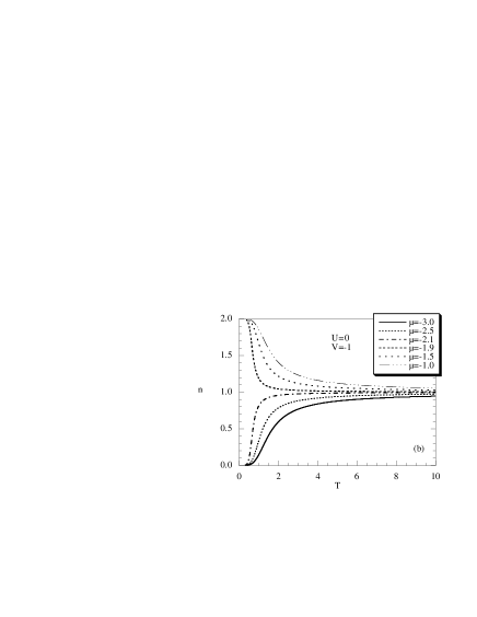
Figure 1: The particle density $n$ is plotted as a function of: (a) the chemical potential at various temperatures for $V=-1$; (b) the temperature at various values of chemical potential for $V=-1$.

We now present some results for the case $U=0$. This situation corresponds to the ionic Hubbard model without local Coulomb interaction, and to the pure spin-1 Ising model, without the crystal field. In one dimension and zero magnetic field, the spin-1 Ising model and the BEG model have been solved exactly by means of the transfer matrix method (Refs. Suzuki et al., 1967; Hintermann and Rys, 1969; Krinsky and Furman, 1975). We recall that the case of zero magnetic field corresponds to the case of half filling in the Hubbard model. The presence of magnetic field has been treated in Ref. Krinsky and Furman, 1975, only for a ferromagnetic coupling and studied only in connection to the existence of critical and tricritical fixed points. The general case of $U$ different from zero will be considered elsewhere. We study the behavior of the system as a function of the parameters $\mu$ and $T$. We take $\left|V\right|=1$: all energies are measured in units of $\left|V\right|$.

At first, we consider the case of an attractive intersite Coulomb potential (i.e., $V<0$). This situations corresponds to $J$ positive (i.e., ferromagnetic coupling). In Fig. 1 (a), we show the particle density $n=<n(i)>=\kappa^{(1)}$ as a function of the chemical potential $\mu$. In terms of the Ising model, this figure should be read as the magnetization $\left\langle S(i)\right\rangle$ versus the magnetic field $h$. By increasing $\mu$, the particle density increases and varies between $0$ and $2$. At $\mu=2V$ we have $n=1$, in agreement with the particle-hole symmetry. By decreasing the temperature, at $\mu=2V$ the system tends to become unstable against a charge ordered state (ferromagnetic order in the Ising model): the particle density jumps from $0$ to $2$. This is also seen in Fig. 1 (b), where the particle density is plotted versus the temperature for various values of the chemical potential. For $\mu<2V$ we have $\lim_{T\rightarrow 0}n=0$, while for $\mu>2V$ we have $\lim_{T\rightarrow 0}n=2$. At zero temperature there is a phase transition at $\mu=2V$ from a state with no particle to a fully occupied state where the charge assumes the maximum value.

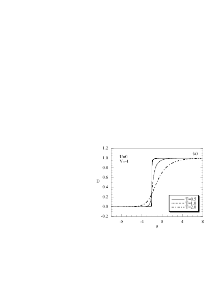
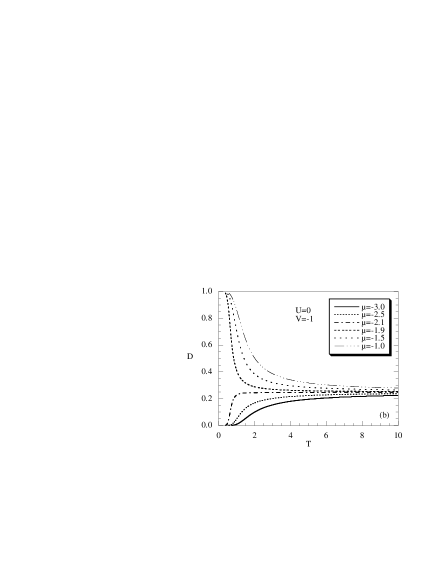
Figure 2: The double occupancy $D$ is plotted as function of: (a) the chemical potential at various temperatures for $V=-1$; (b) the temperature at various values of chemical potential for $V=-1$.

The double occupancy $D$ can be computed by means of the expression

$$D=\frac{n}{2}-C_{11}^{\eta\eta}$$ (87)

The behavior of $D$ is shown in Figs. 2 (a) and 2 (b), where $D$ is given as a function of the chemical potential and temperature, respectively. By increasing $\mu$, the double occupancy increases and varies between 0 and 1. For $\mu<2V$ we have $\lim_{T\rightarrow 0}n=0$, while for $\mu>2V$ we have $\lim_{T\rightarrow 0}D=1$. At zero temperature there is a phase transition at $\mu=2V$ from a state where all the sites are empty to a state where all the sites are doubly occupied. The behavior of the parameters $\kappa^{(p)}$ and $\lambda^{(p)}$ as functions of $\mu$ is similar to that exhibited by $n$; for $T=0$ these parameters at $\mu=2V$ jump from $0$ to their ergodic value.

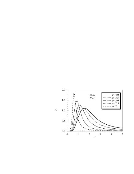
Figure 3: The specific heat $C$ is plotted as a function of the temperature at various values of chemical potential for $V=-1$.

The specific heat is given by

$$C=\frac{dE}{dT}$$ (88)

where the internal energy $E$ can be calculated by means of the expression

$$E=-\mu n+UD+2V\lambda^{(1)}$$ (89)

The specific heat satisfies the property $C(\mu)=C(2V-\mu)$. Therefore, we can limit the analysis to the region $2V<\mu<\infty$ (or $-\infty<\mu<2V$ ). As shown in Fig. 3, the specific heat increases by increasing $T$ up to a certain temperature, then decreases and goes to zero in the limit $T\rightarrow\infty$. Near the transition point $\mu=2V$, the peak is sharper and is situated in the low-temperature region. By moving away from $\mu=2V$, the peak becomes broader and moves to high temperatures.

The thermal compressibility $\kappa^{T}$ is given by

$$\kappa^{T}=\frac{1}{n^{2}}\frac{dn}{d\mu}$$ (90)

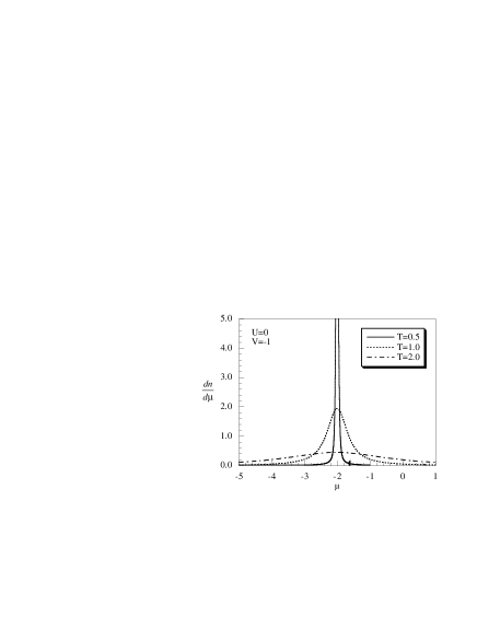
Figure 4: The derivative of the particle density with respect to the chemical potential $dn/d\mu$ is plotted as a function of the chemical potential at various temperatures for $V=-1$.

In Fig. 4 $\frac{dn}{d\mu}$ is plotted versus the chemical potential for various values of temperature. A peak is observed at the transition point $\mu=2V$. By decreasing $T$, the height of the peak increases and the compressibility tends to diverge in the limit $T\rightarrow 0$. As a function of the temperature ($\kappa^{T}$ $)_{\mu=2V}$ exponentially diverges at low temperatures and decreases as $\frac{1}{T}$ in the limit of large T. In terms of the Ising model, Fig. 4 should be read as the spin susceptibility versus the magnetic field.

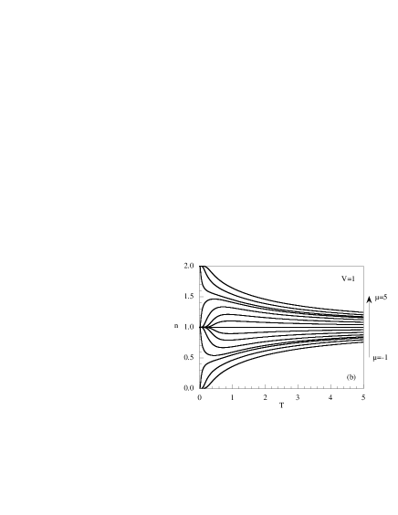
Figure 5: The particle density $n$ is plotted as a function of: (a) the chemical potential at various temperatures for $V=1$; (b) the temperature at various values of the chemical potential for $V=1$.

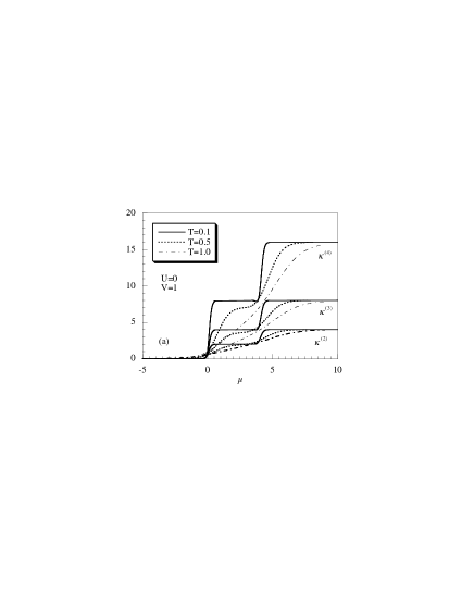
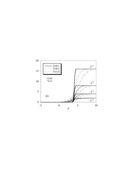
Figure 6: The internal parameters (a) $\kappa^{(2)}$, $\kappa^{(3)}$, $\kappa^{(4)}$ and (b) $\lambda^{(1)}$, $\lambda^{(2)}$, $\lambda^{(3)}$, $\lambda^{(4)}$ are plotted as functions of the chemical potential at various temperatures for $V=1$.

Next, we consider the case of a repulsive intersite Coulomb interaction (i.e., $V>0$). This case corresponds to $J$ negative (i.e., antiferromagnetic coupling). In Fig. 5 (a) we show the particle density $n$ as a function of the chemical potential $\mu$. By increasing $\mu$, the particle density increases from zero, reaches the value $1$ at $\mu=2V$, and tends to $2$ for larger values of the chemical potential. When the temperature decreases some instabilities of the homogeneous phase appear. In the limit $T\rightarrow 0$, two singularities manifest: one at $\mu=0$, where $n$ jumps from $0$ to $1$, the other at $\mu=4V$, where $n$ jumps from $1$ to $2$. In the region $0<\mu<4V$, $n$ exhibits a plateau centered at $\mu=2V$. This behavior is also seen in Fig. 5 (b), where the particle density $n$ is given as a function of the temperature. At $T=0$ we have two phase transitions. At $\mu=0$ the system passes from a state with no charge to a state where the charge is distributed in a checkerboard structure. At $\mu=4V$ there is a second phase transition where the system passes from the checkerboard structure to a state where the charge is uniformly distributed. The checkerboard structure is clearly seen from the behavior of the parameters $\kappa^{(p)}$ and $\lambda^{(p)}$, as shown in Figs. 6. While the parameters $\kappa^{(p)}$ have the same behavior as $n$, with two singularities at $\mu=0$ and at $\mu=4V$, the parameters $\lambda^{(p)}$ exhibit only one singularity at $\mu=4V$. The reason of this difference is related to the fact that $\kappa^{(p)}$ are correlation functions between the site $\mathbf{i}$ and second-nearest neighboring sites, while $\lambda^{(p)}$ mainly relate the site $\mathbf{i}$ to first-nearest neighboring sites.

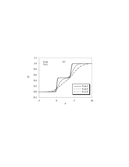
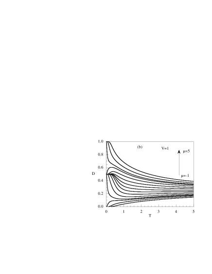
Figure 7: The double occupancy $D$ is plotted as function of: (a) the chemical potential at various temperatures for $V=1$; (b) the temperature at various values of chemical potential for $V=1$.

The double occupancy as a function of the chemical potential is shown in Fig. 7 (a); by increasing $\mu$, $D$ increases from zero and tends to $1$ for large values of the chemical potential. At $T=0$, as also seen in Fig. 7 (b), $D$ has a discontinuity at $\mu=0$, where jumps from zero to $1/2$, and another discontinuity at $\mu=4V$ where jumps from $1/2$ to $1$. In the region $0<\mu<4V$ D has the constant value of $1/2$. Again, this show the transition to a checkerboard structure of the charge.

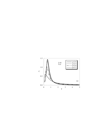
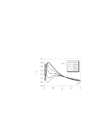
Figure 8: The specific heat $C$ is plotted as a function of the temperature at various values of chemical potential for $V=1$: (a) in the region $2V<\mu<4V$; (b) near the transition point $\mu=4V$; (c) in the region $\mu>4V$.

To study the specific heat, let us distinguish the two regions $2V<\mu<4V$ and $\mu>4V$. In the first region, see Fig. 8 (a), the specific heat increases with temperature, exhibits a peak at a certain temperature $T=T_{1}$, then decreases. When $\mu$ approaches the critical value $\mu_{c}=4V$, see Fig. 8 (b), the specific heat develops a double peak structure with a broad peak at higher temperature than $T_{1}$. The latter temperature decreases with $\mu$ and tends to zero for $\mu\rightarrow\mu_{c}$. It is characteristic of this region the fact that all the specific curves cross at the same temperature, independently on the value of $\mu$. The crossing temperature is $T^{*}\approx 1.1$. The fact that there is a crossing point in the specific heat curves versus $T$, when plotted for different values of some thermodynamics quantities, has been observed in a large variety of systems Vollhardt (1997); Mancini et al. (1999); Mancini and Avella (2004). In the second region, see Fig. 8 (c), C exhibits a low-temperature peak at a certain temperature $T=T_{2}$. $T_{2}$ tends to zero for $\mu\rightarrow\mu_{c}$, increases by increasing $\mu$. Again, close to $\mu_{c}$ there is a double-peak structure, which disappears when $\mu$ moves away from $\mu_{c}$. It is characteristic of this region that no crossing point is observed. For large value of $T$, the two specific heats (i.e. attractive and repulsive $V$) tend to coincide. This is because the system is in a homogeneous phase, where the thermal energy predominates over the Coulomb interaction. It is interesting to observe that the crossing point is observed only for $V>0$ and in the region $0<\mu<4V$, where the checkerboard order is observed.

Figure 9: The derivative of the particle density with respect to the chemical potential $dn/d\mu$ is plotted as a function of the chemical potential at various temperatures for $V=1$.

The thermal compressibility $\kappa^{T}$ is studied in Fig. 9, where $\frac{dn}{d\mu}$ is given as a function of the chemical potential for various values of temperature. When $T$ is lowered a double peak structure develops, with peaks localized at $\mu=0$ and $\mu=4V$. The heights of the peaks increases by decreasing $T$ and tends to diverge in the limit $T\rightarrow 0$. It is worth noticing that for low temperature the compressibility is very small (zero in the limit $T\rightarrow 0$) in the wide region $0<\mu<4V$, where the phase with checkerboard order of the charge is observed. Similar results have been obtained in Ref. Zhang et al., 2004, where the $t-V$ model has been studied within a cluster approximation.

VII Conclusions

The Hubbard model with intersite Coulomb interaction has been studied in the ionic limit (i.e., no kinetic energy). This model is isomorphic to the spin-1 Ising model in presence of a crystal field and an external magnetic field. A finite complete set of eigenoperators and eigenvalues of the Hamiltonian has been found for arbitrary dimensions. This knowledge allows us to determine analytical expressions of the local Green’s functions and the correlation functions. As the eigenoperators do not satisfy a canonical algebra, the GF and the CF depend on a set of unknown parameters, not calculable by means of the dynamics. By using appropriate boundary conditions and algebraic relations we have determined these parameters for the case of an infinite homogeneous chain. Some results for the case $U=0$ (i.e., no local Coulomb interaction / no crystal field) have been given. The system exhibits a different behavior according to the sign of $V$, the intersite Coulomb interaction, or the sign of $J$, the exchange interaction. For $V<0$ ($J>0$, ferromagnetic coupling) at $\mu=2V$ ($h=0$) the system exhibits a phase transition to a charge ordered state (ferromagnetic phase for the Ising model) at zero temperature. For positive $V$ ($J<0$, antiferromagnetic coupling), the system exhibits instabilities at $\mu=0$ ($h=-2\left|J\right|$) and at $\mu=4V$ ($h=2\left|J\right|$). In the limit of zero temperature a phase transition to a state with a checkerboard order of the charge (antiferromagnetic phase for the Ising model) is observed at $\mu=0$. This order persists up to $\mu=4V$, where a second transition to an homogeneous charge order is observed. A crossing point in the specific heat curves is observed only for $V>0$ and in the region $0<\mu<4V$, where the checkerboard order is observed. In the entire region $0<\mu<4V$, the compressibility vanishes at low temperatures. Further study, in particular for the case of finite $U$, will be presented elsewhere.

Appendix A Algebraic relations

Let us start by observing that because of the basic anticommutating rules (3) the number $n(i)=c^{{\dagger}}(i)c(i)$ and the double occupancy $D(i)=n(i)[n(i)-1]/2$ operators satisfy $for\;p\geq 1$ the following algebra

$$\begin{array}[]{l}n^{p}(i)=n(i)+a_{p}D(i)\\ D^{p}(i)=D(i)\\ n^{p}(i)D(i)=2^{p}D(i)\end{array}\;\;\;\;\;\;a_{p}=2^{p}-2$$ (91)

From this algebra several and important relations can be derived. Firstly, let us consider the operator

$$n^{\alpha}(i)=\frac{1}{2d}\stackrel{{\scriptstyle 2d}}{{\sum_{m=1}}}n(\mathbf{i}_{m})$$ (92)

where $\mathbf{i}_{m}$ are the first neighbors of the site $\mathbf{i}$. A basic relation can be derived for the operator $[n^{\alpha}(i)]^{p}$, with $p\geq 1$. In this and in the following Appendices we shall present results for the one-dimensional system . We start from the equation

$$[n^{\alpha}(i)]^{p}={\frac{1}{{2^{p}}}}\sum\limits_{m=0}^{p}{}\left(\begin{array}[]{c}p\\ m\end{array}\right)n(i_{1})^{p-m}n(i_{2})^{m}$$ (93)

Because of the algebraic relations (91) we obtain

$$[n^{\alpha}(i)]^{p}={\frac{1}{{2^{p}}}}\sum\limits_{m=1}^{4}{}b_{m}^{(p)}Z_{m}$$ (94)

where the operators $Z_{m}$ are defined as

$$\begin{array}[]{l}{Z_{1}=2n^{\alpha}(i)}\\ {Z_{2}=2D^{\alpha}(i)+n(i_{1})n(i_{2})}\\ {Z_{3}=D(i_{1})n(i_{2})+D(i_{2})n(i_{1})}\\ {Z_{4}=D(i_{1})D(i_{2})}\end{array}$$ (95)

and the coefficients $b_{m}^{(p)}$ have the expressions

$$\begin{array}[]{l}{b_{1}^{(p)}=1}\\ {b_{2}^{(p)}=\sum\limits_{m=1}^{p-1}{}\left(\begin{array}[]{c}p\\ m\end{array}\right)=2(-1+2^{p-1})}\\ {b_{3}^{(p)}=\sum\limits_{m=1}^{p-1}{}\left(\begin{array}[]{c}p\\ m\end{array}\right)a_{p-m}=3(1-2^{p}+3^{p-1})}\\ {b_{4}^{(p)}=\sum\limits_{m=1}^{p-1}{}\left(\begin{array}[]{c}p\\ m\end{array}\right)a_{p-m}a_{m}=4(-1+3\cdot 2^{p-1}-3^{p}+4^{p-1})}\end{array}$$ (96)

By solving the system (94) with respect to the variables $Z_{m}$, we can obtain from (94) the recurrence rule

$$[n^{\alpha}(i)]^{p}=\sum\limits_{m=1}^{4}{}A_{m}^{(p)}[n^{\alpha}(i)]^{m}$$ (97)

where the coefficients $A_{m}^{(p)}$ are defined as

$$\begin{array}[]{l}{A_{1}^{(p)}={\frac{1}{{2^{p-1}}}}[b_{1}^{(p)}-{\frac{1}{2}}b_{2}^{(p)}+{\ \frac{1}{3}}b_{3}^{(p)}-{\frac{1}{4}}b_{4}^{(p)}]}\\ {A_{2}^{(p)}={\frac{1}{{2^{p-1}}}}[b_{2}^{(p)}-b_{3}^{(p)}+{\frac{{11}}{{12}}}b_{4}^{(p)}]}\\ {A_{3}^{(p)}={\frac{1}{{2^{p-1}}}}[{\frac{2}{3}}b_{3}^{(p)}-b_{4}^{(p)}]}\\ {A_{4}^{(p)}={\frac{1}{{2^{p-1}}}}{\frac{1}{3}}b_{4}^{(p)}}\end{array}$$ (98)

We note that

$$\sum\limits_{m=1}^{4}{}A_{m}^{(p)}=1$$ (99)

In Table 1 we give some values of the coefficients $A_{m}^{(p)}.$

$p$ $A_{1}^{(p)}$ $A_{2}^{(p)}$ $A_{3}^{(p)}$ $A_{4}^{(p)}$ $1$ $1$ $0$ $0$ $0$ $2$ $0$ $1$ $0$ $0$ $3$ $0$ $0$ $1$ $0$ $4$ $0$ $0$ $0$ $1$ $5$ $-\frac{3}{2}$ $\frac{25}{4}$ $-\frac{35}{4}$ $5$ $6$ $-\frac{15}{2}$ $\frac{119}{4}$ $-\frac{75}{2}$ $\frac{65}{4}$ $7$ $-\frac{195}{8}$ $\frac{1505}{16}$ $-\frac{1799}{16}$ $\frac{175}{4}$ $8$ $-\frac{525}{8}$ $\frac{3985}{16}$ $-\frac{1155}{4}$ $\frac{1701}{16}$

Appendix B The energies matrices

The energy matrices $\epsilon^{(\xi)}$ and $\epsilon^{(\eta)}$ can be calculated by means of the equations of motion (19) and (20) and the recurrence rule (21). The explicit expressions are

$$\varepsilon^{(\xi)}=\left(\begin{array}[]{ccccc}{-\mu}&{2dV}&{\cdots}&0&0\\ 0&{-\mu}&{\cdots}&0&0\\ \vdots&\vdots&\vdots&\vdots&\vdots\\ 0&0&{\cdots}&{-\mu}&{2dV}\\ 0&{{{2dVA_{1}^{(4d+1)}}}}&{\cdots}&{{{2dVA_{4d-1}^{(4d+1)}}}}&{{{-\mu+2dVA_{4d}^{(4d+1)}}}}\end{array}\right)$$ (100)

$$\varepsilon^{(\eta)}=\left(\begin{array}[]{ccccc}U{-\mu}&{2dV}&{\cdots}&0&0\\ 0&U{-\mu}&{\cdots}&0&0\\ \vdots&\vdots&\vdots&\vdots&\vdots\\ 0&0&{\cdots}&U{-\mu}&{2dV}\\ 0&{{{2dVA_{1}^{(4d+1)}}}}&{\cdots}&{{{2dVA_{4d-1}^{(4d+1)}}}}&U{{{\ -\mu+2dVA_{4d}^{(4d+1)}}}}\end{array}\right)$$ (101)

where ${{{A_{m}^{(4d+1)}}}}$ are the coefficients appearing in (19). In particular, for one dimension

$$\epsilon^{(\xi)}=\left(\begin{array}[]{ccccc}-\mu&2V&0&0&0\\ 0&-\mu&2V&0&0\\ 0&0&-\mu&2V&0\\ 0&0&0&-\mu&2V\\ 0&-3V&\frac{25V}{2}&-\frac{35}{2}V&-\mu+10V\end{array}\right)$$ (102)

$$\epsilon^{(\eta)}=\left(\begin{array}[]{ccccc}U-\mu&2V&0&0&0\\ 0&U-\mu&2V&0&0\\ 0&0&U-\mu&2V&0\\ 0&0&0&U-\mu&2V\\ 0&-3V&\frac{25V}{2}&-\frac{35}{2}V&U-\mu+10V\end{array}\right)$$ (103)

The matrices $\Omega^{(\xi)}$ and $\Omega^{(\eta)}$ have the expressions

$$\Omega^{(\xi)}=\Omega^{(\eta)}=\left(\begin{array}[]{ccccc}1&2^{4}&1&(2/3)^{4}&(1/2)^{4}\\ 0&2^{3}&1&(2/3)^{3}&(1/2)^{3}\\ 0&2^{2}&1&(2/3)^{2}&(1/2)^{2}\\ 0&2&1&(2/3)&(1/2)\\ 0&1&1&1&1\end{array}\right)$$ (104)

Appendix C The spectral density matrices

By means of the formulas (34) and recalling the expressions [see Appendix B] for the energy matrices, and the expressions (31)-(32) of the normalization matrix, we can easily calculate the spectral matrices. Furthermore, we note that the matrices $\Omega^{(\xi)}$ and $\Omega^{(\eta)}$ are equal. Then, the spectral density matrices have similar form in terms of the matrix elements of the normalization matrices. Because of the recurrence relation, we need to calculate only the first row of the matrices. Calculations show that the matrices $\sigma^{(a,n)}$ have the following form

$$\sigma^{(a,n)}=\Sigma_{n}^{(a)}\Gamma^{(n)}\qquad n=1,2.\cdots,4d+1$$ (105)

where $\Sigma_{n}^{(a)}$ are functions of the elements $I_{1,m}^{(a)}$ $(m=1,2.\cdots,4d+1)$ and $\Gamma^{(n)}$ are matrices of rank $(4d+1)\times(4d+1)$. For the one-dimensional case

$$\begin{array}[]{l}{\Sigma_{1}^{(a)}={\frac{1}{6}}(6I_{1,1}^{(a)}-25I_{1,2}^{(a)}+35I_{1,3}^{(a)}-20I_{1,4}^{(a)}+4I_{1,5}^{(a)})}\\ {\Sigma_{2}^{(a)}={\frac{4}{3}}(6I_{1,2}^{(a)}-13I_{1,3}^{(a)}+9I_{1,4}^{(a)}-2I_{1,5}^{(a)})}\\ {\Sigma_{3}^{(a)}=-6I_{1,2}^{(a)}+19I_{1,3}^{(a)}-16I_{1,4}^{(a)}+4I_{1,5}^{(a)}}\\ {\Sigma_{4}^{(a)}={\frac{4}{3}}(2I_{1,2}^{(a)}-7I_{1,3}^{(a)}+7I_{1,4}^{(a)}-2I_{1,5}^{(a)})}\\ {\Sigma_{5}^{(a)}={\frac{1}{6}}(-3I_{1,2}^{(a)}+11I_{1,3}^{(a)}-12I_{1,4}^{(a)}+4I_{1,5}^{(a)})}\end{array}$$ (106)

$$\begin{array}[]{l}\Gamma_{1,m}^{(1)}=(\begin{array}[]{lllll}1&0&0&0&0\end{array})\\ \Gamma_{1,m}^{(2)}=(\begin{array}[]{lllll}1&2^{-1}&2^{-2}&2^{-3}&2^{-4}\end{array})\\ \Gamma_{1,m}^{(3)}=(\begin{array}[]{lllll}1&1&1&1&1\end{array})\\ \Gamma_{1,m}^{(4)}=(\begin{array}[]{lllll}1&(2/3)^{-1}&(2/3)^{-2}&(2/3)^{-3}&(2/3)^{-4}\end{array})\\ \Gamma_{1,m}^{(5)}=(\begin{array}[]{lllll}1&(1/2)^{-1}&(1/2)^{-2}&(1/2)^{-3}&(1/2)^{-4}\end{array})\end{array}$$ (107)

References

- Mancini (2005a) F. Mancini, Europhys. Lett. 70, 1 (2005a).
- Seo and Fukuyama (1998) H. Seo and H. Fukuyama, J. Phys. Soc. Jpn. 77, 2602 (1998).
- van Dongen (1994) P. van Dongen, Phy. Rev. B 50, 14016 (1994).
- Pietig et al. (1999) R. Pietig, R. Bulla, and S. Blawid, Phys. Rev. Lett. 82, 4046 (1999).
- McKenzie et al. (2001) R. H. McKenzie et al., Phys. Rev. B 64, 085109 (2001).
- Merino and McKenzie (2001) J. Merino and R. H. McKenzie, Phys. Rev. Lett. 87, 237002 (2001).
- Hoang and Thalmeier (2002) A. Hoang and P. Thalmeier, J. Phys. Condens. Matter 14, 6639 (2002).
- Hirsch (1984) J. Hirsch, Phys. Rev. Lett. 53, 2327 (1984).
- Hellberg (2001) C. Hellberg, J. Appl. Phys. 89, 6627 (2001).
- Calandra et al. (2002) M. Calandra, J. Merino, and R. H. McKenzie, Phys. Rev. B 66, 195102 (2002).
- Blume (1966) M. Blume, Phys. Rev. 141, 517 (1966).
- Capel (1966) H. W. Capel, Physica (Utrecht) 32, 966 (1966).
- Capel (1967a) H. W. Capel, Physica (Utrecht) 33, 295 (1967a).
- Capel (1967b) H. W. Capel, Physica (Utrecht) 37, 423 (1967b).
- Blume et al. (1971) M. Blume, V. J. Emery, and R. D. Griffiths, Phys. Rev. A 4, 1071 (1971).
- Furman et al. (1977) D. Furman, S. Dattagupta, and R. B. Griffiths, Phys. Rev. B 15, 441 (1977).
- Suzuki et al. (1967) M. Suzuki, B. Tsujiyama, and S. Katsura, J. Math. Phys. 8, 124 (1967).
- Hintermann and Rys (1969) A. Hintermann and F. Rys, Helv. Phys. Acta 42, 608 (1969).
- Obokata and Oguchi (1968) T. Obokata and T. Oguchi, J. Phys. Soc. Jpn 25, 322 (1968).
- Chakraborty and Tucker (1986) K. G. Chakraborty and J. W. Tucker, J. Magn. Matter 54-57, 1349 (1986).
- Rosengren and Haggkvist (1989) A. Rosengren and R. Haggkvist, Phys. Rev. Lett. 63, 660 (1989).
- Bernasconi and Rys (1971) J. Bernasconi and F. Rys, Phys. Rev. B 4, 3045 (1971).
- Mukamel and Blume (1974) D. Mukamel and M. Blume, Phys. Rev. A 10, 610 (1974).
- Lajzerowicz and Sivardi re (1975) J. Lajzerowicz and J. Sivardi re, Phys. Rev. A 11, 2079 (1975).
- Sivardi re and Lajzerowicz (1975a) J. Sivardi re and J. Lajzerowicz, Phys. Rev. A 11, 2090 (1975a).
- Sivardi re and Lajzerowicz (1975b) J. Sivardi re and J. Lajzerowicz, Phys. Rev. A 11, 2101 (1975b).
- Hoston and Berker (1991) W. Hoston and A. N. Berker, Phys. Rev. Lett. 67, 1027 (1991).
- Riedel and Wegner (1974) E. K. Riedel and F. J. Wegner, Phys. Rev. B 9, 294 (1974).
- Berker and Wortis (1976) A. N. Berker and M. Wortis, Phys. Rev. B 14, 4946 (1976).
- Burkhardt (1976) T. W. Burkhardt, Phys. Rev. B 14, 1196 (1976).
- Burkhardt and Knops (1977) T. W. Burkhardt and H. J. F. Knops, Phys. Rev. B 15, 1602 (1977).
- Mahan and Girvin (1978) G. D. Mahan and S. M. Girvin, Phys. Rev. B 17, 4411 (1978).
- Kaufman et al. (1981) M. Kaufman, R. B. Griffiths, J. M. Yeomans, and M. Fisher, Phys. Rev. B 23, 3448 (1981).
- Yeomans and Fisher (1981) J. M. Yeomans and M. E. Fisher, Phys. Rev. B 24, 2825 (1981).
- Oitmaa (1972) J. Oitmaa, J. Phys. C 5, 435 (1972).
- Fox and Gaunt (1972) P. F. Fox and D. S. Gaunt, J. Phys. C 5, 3085 (1972).
- Saul and Wortis (1974) D. M. Saul and M. Wortis, Phys. Rev. B 9, 4964 (1974).
- Lock and Lee (1984) S. L. Lock and B. S. Lee, Phys. Status Solidi B 124, 593 (1984).
- Tanaka and Kawabe (1985) M. Tanaka and T. Kawabe, J. Phys. Soc. Jpn. 54, 2194 (1985).
- Wang and Wentworth (1987) L. Wang and C. Wentworth, J. Appl. Phys. 61, 4411 (1987).
- Wang et al. (1987) L. Wang, F. Lee, and J. D. Kimel, Phys. Rev. B 36, 8945 (1987).
- Rachadi and Benyoussef (2003) A. Rachadi and A. Benyoussef, Phys. Rev. B 68, 064113 (2003).
- Grollau et al. (2001) S. Grollau, E. Kierlik, M. L. Rosinberg, and G. Tarjus, Phys. Rev. E 63, 041111 (2001).
- Grollau (2002) S. Grollau, Phys. Rev. E 65, 056130 (2002).
- Krinsky and Furman (1975) S. Krinsky and D. Furman, Phys. Rev. B 11, 2602 (1975).
- Mi and Yang (1994) X. D. Mi and Z. R. Yang, Phys. Rev. E 49, 3636 (1994).
- Doman and ter Haar (1962) B. G. S. Doman and D. ter Haar, Phys. Lett. 2, 15 (1962).
- Tahir-Kheli et al. (1963) R. A. Tahir-Kheli, B. G. S. Doman, and D. ter Haar, Phys. Lett. 4, 5 (1963).
- Doman (1963) B. G. S. Doman, Phys. Lett. 4, 156 (1963).
- Callen (1963) H. B. Callen, Phys. Lett. 4, 161 (1963).
- Suzuki (1965) M. Suzuki, Phys. Lett. 19, 267 (1965).
- Oguchi and Ono (1966) T. Oguchi and I. Ono, Prog. Theor. Phys. 35, 998 (1966).
- Tyablikov and Fedyanin (1967) S. V. Tyablikov and V. K. Fedyanin, Fisika metallov and metallovedenie 23, 193 (1967).
- Tahir-Kheli (1968) R. A. Tahir-Kheli, Phys. Rev. 169, 517 (1968).
- Kalashnikov and Fradkin (1969) O. K. Kalashnikov and E. S. Fradkin, Sov. Phys. JETP 28, 976 (1969).
- Anderson (1971) F. B. Anderson, Phys. Rev. B 3, 3950 (1971).
- Taggart (1979) G. B. Taggart, Phys. Rev. B 20, 3886 (1979).
- Honmura and Kaneyoshi (1978) R. Honmura and T. Kaneyoshi, Prog. Theor. Phys. 60, 635 (1978).
- Siqueira and Fittipaldi (1985) A. F. Siqueira and I. P. Fittipaldi, Phys. Rev. B 31, 6092 (1985).
- Mancini and Avella (2003) F. Mancini and A. Avella, Eur. Phys. J. B 37, 37 (2003).
- Mancini (2003) F. Mancini, in Highlights in Condensed Matter Physics, edited by A. Avella, R. Citro, C. Noce, and M. Salerno (American Institute of Physics, New York, 2003), pp. 240–257.
- Mancini and Avella (2004) F. Mancini and A. Avella, Advances in Physics 53, 537 (2004).
- Mancini (1998) F. Mancini, Physics Letters A 249, 231 (1998).
- Mancini (2005b) F. Mancini, Eur. Phys. J. B 45, 497 (2005b).
- Fedro (1976) A. J. Fedro, Phys. Rev. B 14, 2983 (1976).
- Vollhardt (1997) D. Vollhardt, Phys. Rev. Lett. 78, 1307 (1997).
- Mancini et al. (1999) F. Mancini, H. Matsumoto, and D. Villani, J. Phys. Studies 3, 474 (1999).
- Zhang et al. (2004) Y. Z. Zhang, T. Minh-Tien, V. Yushankhai, and P. Thalmeier (2004), cond-mat/0411539.
- Mancini (2005c) F. Mancini, Tech. Rep., University of Salerno (2005c).