Multiple Core-Hole Coherence in X-Ray Four-Wave-Mixing Spectroscopies

Abstract

Correlation-function expressions are derived for the coherent nonlinear response of molecules to three resonant ultrafast pulses in the x-ray regime. The ability to create two-core-hole states with controlled attosecond timing in four-wave-mixing and pump probe techniques should open up new windows into the response of valence electrons, which are not available from incoherent x-ray Raman and fluorescence techniques. Closed expressions for the necessary four-point correlation functions are derived for the electron-boson model by using the second order cumulant expansion to describe the fluctuating potentials. The information obtained from multidimensional nonlinear techniques could be used to test and refine this model, and establish an anharmonic oscillator picture for electronic excitations.

I Introduction

The development of bright attosecond soft and hard x-ray sources such as the free electron laser has triggered considerable interest in all-x-ray nonlinear spectroscopymurnane91 ; krausz ; cherguireview ; cherguimukamelpreface . In resonant optical techniques in the visible, a photon is tuned to high frequency ($\sim 2$eV) electronic transitions, but a wealth of information is provided on lower-frequency ($<0.4$eV) nuclear (vibrational and phonon) degrees of freedom which are accessible through multiphoton (e.g. Raman-type) resonances with differences (and higher combinations) of visible photons. In a completely analogous manner, combinations of x-ray photons resonant with high frequency ( keV) core transitions can probe the lower frequency ($<50$eV) valence electronic excitations. By exploiting this analogy, we can use the theoretical apparatus developed for probing electronic and vibrational coherences in nonlinear opticsmukbook , to predict nonlinear x-ray signals and design new multiple pulse experiments. For example, the concepts underlying multidimensional techniquessmannreview which provide extremely valuable information on optical excitations in molecular aggregates can be extended to probe correlations among multiple core hole states.

Nozieres and De Dominicis had proposed a model Hamiltonian for resonant x-ray processes in metalsnozieres69 . The $\sim\omega^{\alpha}$ threshold (Fermi edge singularity) behavior of x-ray absorption was calculated. The interplay of the large number of electron hole pairs and the vanishing of the many-electron wavefunction overlap with and without the core hole (Anderson’s Catastrophe) can result in either a diverging ($\alpha<0$) or converging ($\alpha>0$) lineshape at threshold, as shown by Mahanmahan82 ; hedin96 ; nordgren97 . Signatures of this singularity in femtosecond optical pump probe spectroscopy of doped semiconductor nanostructures have been studied.perakis Higher order radiative processes such as spontaneous emission (fluorescence or Raman) or nonlinear wave mixing provide more detailed insights through multipoint correlation functionsnozieresandabrams ; beyondoneelectronmodel ; mukbook ; agrenreview99 ; agren01 . The formal theory of x-ray response closely resembles its visible or infrared counterpart where the relevant correlation and response functions and possible time orderings have been studied extensively.mukxraypaper It is also closely connected with the treatment of currents in open molecular systems coupled to electrodes.upendra

In this paper we apply the density matrix Liouville space formalismmukbook to calculate time resolved x-ray four-wave mixing signals and compare them with spontaneous emission and pump probe spectroscopy. Much current activity is focused on the application of time resolved diffraction to probe structural changes such as surface melting.melting From a theoretical point these can be described using the existing formalism of diffraction by simply including the parametric time dependence of the electronic charge density; coherence does not play a role in these techniques. Other experiments have been carried out using a visible or an infrared pump followed by the absorption of an x-ray probe. These techniques provide x-ray snapshots of vibrational coherence or coherence among valence electronic states. agren05 Photoelectron spectroscopy provides additional novel ultrafast probes.agren04 ; gelmukhanov05

Pure resonant x-ray nonlinear optics of the type considered here can probe high frequency coherence of many-electron states involving core hole transitions and provide multidimensional real space pictures for the response of valence electrons to external perturbations. The necessary multipoint correlation functions may be calculated using several levels of theory. (i) Multiple summations over the many electron states of the valence system with $N$, $N+1$, and $N+2$ electrons in the presence of zero, one, and two core holes respectively. (ii) The transition potential method, which uses a reference system with partially filled orbitals degroottransstate ; nexafsofadsorbates ; dftinnershell ; degroot74 (iii) many-body Green function perturbative techniques. nozieresandabrams ; agren01 ; beyondoneelectronmodel ; hedin99 ; hedin96 ; nordgren97 ; cederbaum81 (iv) Replace the original Hamiltonian by the electron-boson model (EBM) and treat charge-density fluctuations as classical oscillations. langreth ; hedin99 ; langreth70 ; lundqvist67 ; overhauser71

Method (i) is conceptually the simplest but the most expensive numerically. The sum over state (SOS) expressions for nonlinear response functions allow us to employ any level of quantum chemistry for computing electronically excited states. TDDFT, for example, provides a relatively efficient way for computing a large number of electronically excited states.gross The relevant states are determined by the pulse bandwidth. e.g. $3.75$eV for a $10$as pulse. Method (ii) Represents systems with different numbers of core holes by varying the occupation numbers of a single set of reference orbitals. This approximate method works well for core level spectroscopies of small molecules, and may be extended to the nonlinear response. Method (iii) was used by Nozieres and coworkers to compute XANES and x-ray Raman spectra.nozieres69 ; nozieresandabrams It is formally exact, and allows the development of powerful approximations. The EBM is by far the simplest to implement, since it is exactly solvable by the second order cumulant expansion. The model is not expected to apply for small molecules where the core electrons added to the valence band by the absorption of an x-ray photon need to be treated explicitly. It has been tested and found to work quite well for solids (semiconductors and metals). Plasmon satellites have been predicted in x-ray photoemission.hedin85 ; hedin96 ; beyondoneelectronmodel and inelastic scattering.schulke They are less clearly seen in x-ray absorption, but have indirect signatures in e.g. the oscillator strengths. Using the EBM, electronic excitations are described as anharmonic oscillations whose parameters may be extracted from coherent nonlinear x-ray techniques.

II The Nonlinear X-Ray Response

We start with the Mahan-Nozieres-De Dominicis(MND) Hamiltonianmahan82 ; nozieres69 ; almbladh01 ; hedin99 ; hedin85

$$H=\sum_{k}\epsilon_{k}c_{k}^{\dagger}c_{k}+\sum_{n}\epsilon_{n}d_{n}^{\dagger}d_{n}+\sum_{\begin{subarray}{c}kk^{\prime}\\ n\end{subarray}}V_{kk^{\prime},n}c_{k}^{\dagger}c_{k^{\prime}}d_{n}d_{n}^{\dagger}$$ (1)

where $c_{k}^{\dagger}$, $d_{n}^{\dagger}$ are the Fermi creation operators for a valence and a core electron respectively, $\epsilon_{n}$ is the energy of core state $n$, and $V_{kk^{\prime},n}$ is the potential acting on the valence electrons due to the $n$th core hole.

The dipole interaction with the x-ray field in the rotating wave approximation (RWA) is

$$H_{int}=\sum_{n}\left[E(\mathbf{r},t)B_{n}^{\dagger}+E^{*}(\mathbf{r},t)B_{n}\right]$$ (2)

where

$$B^{\dagger}_{n}=\sum_{k}\mu_{kn}c_{k}^{\dagger}d_{n},\qquad B_{n}=\sum_{k}\mu_{nk}c_{k}d^{\dagger}_{n}$$ (3)

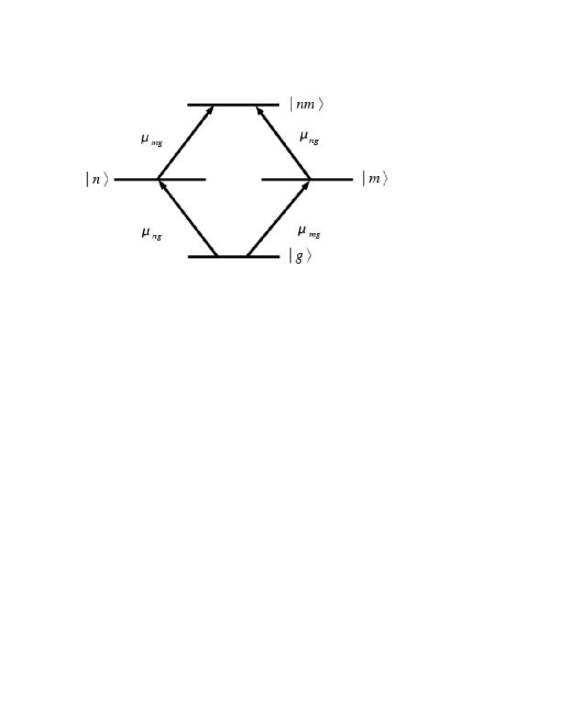
Figure 1: The core exciton states which enter the third order response. $|g\rangle$ is the ground state, $|n\rangle$ and $|m\rangle$ are single core-hole states, and $|nm\rangle$ is a double core hole state.

are creation (annihilation) operators for core-hole excitons. $\mu_{kn}$ is the dipole matrix element between the $n$’th core orbital and the $k$’th valence orbital, and $E(\mathbf{r},t)$ is the complex field envelope (see Eq. (25)). The possible transitions between the zero, one and two core hole states are shown in Fig. 1.

The $j$’th order molecular response to the x-ray field is described by the induced polarization mukbook :

$$P^{(j)}(\mathbf{r},t)\equiv Tr(\hat{P}\hat{\rho}^{(j)}(t))$$ (4)

where $Tr(\ldots)$ denotes the trace and

$$\hat{P}=\sum_{n}(B_{n}+B^{\dagger}_{n})$$ (5)

is the polarization operator. $\hat{\rho}^{(j)}(t)$ is the density matrix describing the state of the molecule obtained by solving the Liouville equation to $j$’th order in the field.

$$\frac{d\hat{\rho}}{dt}=-i[\hat{H},\hat{\rho}],$$ (6)

where the total Hamiltonian $\hat{H}=\hat{H}_{0}+\hat{H}_{int}$, $\hat{H}_{0}$ is the material Hamiltonian.

Eq. (4) can be expanded as

$$P^{(j)}(\mathbf{r},t) = \int_{0}^{\infty}dt_{n}\int_{0}^{\infty}dt_{n-1}\ldots\int_{0}^{\infty}dt_{1}S^{(j)}(t_{n},t_{n-1},\ldots,t_{1})\times$$ (7)

$$E(\mathbf{r},t-t_{n})E(\mathbf{r},t-t_{n}-t_{n-1})\ldots E(\mathbf{r},t-t_{n}-t_{n-1}\ldots-t_{1}).$$

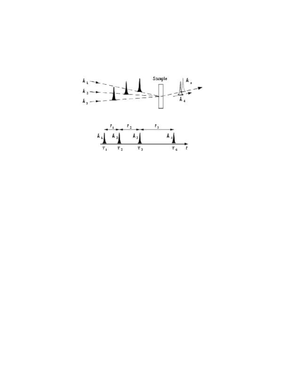
Figure 2: (Upper panel) Laser pulse sequence in a three-pulse, four-wave mixing experiment. Three pulses $\mathbf{k}_{1}$, $\mathbf{k}_{2}$ and $\mathbf{k}_{3}$ create the nonlinear polarization in the sample, which generates the new x-ray field in the direction $\mathbf{k}_{s}=\pm\mathbf{k}_{1}\pm\mathbf{k}_{2}\pm\mathbf{k}_{3}$. $\mathbf{k}_{4}=\mathbf{k}_{s}$ is the heterodyne field. (Lower panel) The peak ordering and time intervals.

where $S^{(j)}(t_{n},t_{n-1},\ldots,t_{1})$ denotes the $j$–th order response function and $t_{n}\equiv\tau_{n+1}-\tau_{n}$ is the time delay between two consecutive interactions with the x-ray field (see Fig. 2).

The first order polarization is related to the linear response function $S^{(1)}$:

$$P^{(1)}(\mathbf{r},t)=\int_{0}^{\infty}dt_{1}S^{(1)}(t_{1})E(\mathbf{r},t-t_{1}),$$ (8)

$S^{(1)}$ is a second rank tensor with respect to the polarization direction. For clarity we do not use tensor notation.

Here

$$S^{(1)}(t_{1})=i\theta(t_{1})[J(t_{1})-J^{\ast}(t_{1})],$$ (9)

$J(t_{1})=\langle\hat{P}(t_{1})\hat{P}(0)\rangle$ is a two point correlation function and the polarization operator is given in the Heisenberg representation:

$$\hat{P}(t_{1})=\exp(i\hat{H}_{0}t_{1})\hat{P}\exp(-i\hat{H}_{0}t_{1}),$$ (10)

$\theta(t)$ is the Heavyside function ($\theta(t)=0$ for $t<0$, $\theta(t)=1$ for $t\geq 0$) which represents causality, and the angular brackets $\langle\cdots\rangle$ denote the trace over the ground state density matrix:

The third order polarization is given by

$$P^{(3)}(\mathbf{r},t) = \int\!\!\!\int\!\!\!\int_{0}^{\infty}dt_{3}dt_{2}dt_{1}S^{(3)}(t_{3},t_{2},t_{1})\times$$ (11)

$${E}(\mathbf{r},t-t_{3}){E}(\mathbf{r},t-t_{3}-t_{2}){E}(\mathbf{r},t-t_{3}-t_{2}-t_{1}).$$

The third order response function is similarly given by a sum of eight terms, each representing a distinct Liouville space pathway mukbook :

$$S(t_{3},t_{2},t_{1})=i^{3}\theta(t_{3})\theta(t_{2})\theta(t_{1})\sum_{p=1}^{4}\Big{[}R_{p}(t_{3},t_{2},t_{1})-R_{p}^{\ast}(t_{3},t_{2},t_{1})\Big{]},$$ (12)

where

$$R_{1}(t_{3},t_{2},t_{1}) = F(t_{1},t_{1}+t_{2},t_{1}+t_{2}+t_{3},0),$$

$$R_{2}(t_{3},t_{2},t_{1}) = F(0,t_{1}+t_{2},t_{1}+t_{2}+t_{3},t_{1}),$$

$$R_{3}(t_{3},t_{2},t_{1}) = F(0,t_{1},t_{1}+t_{2}+t_{3},t_{1}+t_{2}),$$

$$R_{4}(t_{3},t_{2},t_{1}) = F(t_{1}+t_{2}+t_{3},t_{1}+t_{2},t_{1},0),$$ (13)

and the four-point correlation function is given by:

$$F(\tau_{4},\tau_{3},\tau_{2},\tau_{1})=\langle\hat{P}(\tau_{4})\hat{P}(\tau_{3})\hat{P}(\tau_{2})\hat{P}(\tau_{1})\rangle.$$ (14)

The polarization may be alternatively expressed in the frequency domain using the susceptibility tensors: $\chi^{(1)}(-\omega_{a};\omega_{a})\equiv\chi^{(1)}(\omega_{a})$ and $\chi^{(3)}(-\omega_{s};\omega_{a},\omega_{b},\omega_{c})$:

$$P^{(1)}(\mathbf{r},t)=\int_{-\infty}^{\infty}d\omega_{a}\exp(-i\omega_{a}t)\chi^{(1)}(\omega_{a})\mathcal{E}(\mathbf{r},\omega_{a}).$$ (15)

$$P^{(3)}(\mathbf{r},t) = \int\!\!\!\int\!\!\!\int\!\!\!\int_{-\infty}^{\infty}d\omega_{s}d\omega_{a}d\omega_{b}d\omega_{c}\exp(-i\omega_{s}t)\times$$ (16)

$$\times\chi^{(3)}(-\omega_{s};\omega_{a},\omega_{b},\omega_{c})\mathcal{E}(\mathbf{r},\omega_{a})\mathcal{E}(\mathbf{r},\omega_{b})\mathcal{E}(\mathbf{r},\omega_{c}).$$

$\mathcal{E}(\mathbf{r},\omega_{a})$ is the x-ray field in the frequency domain:

$${\mathcal{E}}(\mathbf{r},\omega)\equiv\int_{-\infty}^{\infty}d\tau{E}(\mathbf{r},\tau)\exp(i\omega\tau).$$ (17)

The response functions and the nonlinear susceptibilities are related by a Fourier transform:

$$\chi^{(1)}(\omega_{a})\equiv\int_{0}^{\infty}dt_{1}S^{(1)}(t_{1})\exp(i\omega_{a}t_{1}),$$ (18)

$$\chi^{(3)}(-\omega_{s};\omega_{a},\omega_{b},\omega_{c})\equiv\frac{1}{3!}\sum_{p}\int\!\!\!\int\!\!\!\int_{0}^{\infty}dt_{3}dt_{2}dt_{1}S^{(3)}(t_{3},t_{2},t_{1})$$ (19)

$$\exp(i(\omega_{a}+\omega_{b}+\omega_{c})t_{3}+i(\omega_{a}+\omega_{b})t_{2}+i\omega_{a}t_{1}),$$

where $\omega_{s}\equiv\omega_{a}+\omega_{b}+\omega_{c}$ and the sum $\sum_{p}$ runs over all $3!=6$ permutations of $\omega_{a},\omega_{b},\omega_{c}$.

III Expansion in Many-Electron Eigenstates

Expressing the two-point correlation function Eq. (9) using Eq. (5) we get

$$J(t)=\sum_{n}\langle B_{n}(t)B_{n}^{\dagger}(0)\rangle$$ (20)

Similarly, upon the substitution of Eq. (5) in Eq. (14) we find three contributions $F=F_{1}+F_{2}+F_{3}$ where

$$F_{1}(\tau_{4},\tau_{3},\tau_{2},\tau_{1}) = \sum_{n,m}\langle B_{m}(\tau_{4})B_{m}^{\dagger}(\tau_{3})B_{n}(\tau_{2})B_{n}^{\dagger}(\tau_{1})\rangle,$$

$$F_{2}(\tau_{4},\tau_{3},\tau_{2},\tau_{1}) = \sum_{n\neq m}\langle B_{n}(\tau_{4})B_{m}(\tau_{3})B_{m}^{\dagger}(\tau_{2})B_{n}^{\dagger}(\tau_{1})\rangle,$$

$$F_{3}(\tau_{4},\tau_{3},\tau_{2},\tau_{1}) = \sum_{n\neq m}\langle B_{m}(\tau_{4})B_{n}(\tau_{3})B_{m}^{\dagger}(\tau_{2})B_{n}^{\dagger}(\tau_{1})\rangle.$$ (21)

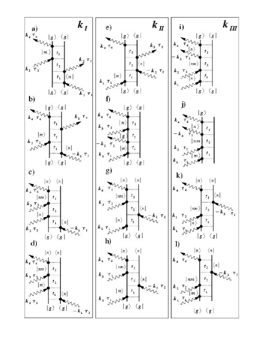
Figure 3: Double-sided Feynman diagams representing the Liouville-space pathways contributing to the third-order response in the rotating wave approximation. The level scheme is given in Fig. 1. Shown are the diagrams contributing to the four-wave mixing signal generated along the various possible directions: $\mathbf{k}_{I}=-\mathbf{k}_{1}+\mathbf{k}_{2}+\mathbf{k}_{3}$, $\mathbf{k}_{II}=\mathbf{k}_{1}-\mathbf{k}_{2}+\mathbf{k}_{3}$, and $\mathbf{k}_{III}=\mathbf{k}_{1}+\mathbf{k}_{2}-\mathbf{k}_{3}$. Diagrams (a), (b), (e), and (f) correspond to $F_{1}$ and only include one-exciton states. All other diagrams also involve two-exciton states. (i), (c), (g), and (k) correspond to $F_{2}$ and (j), (d), (h) and (l) represent $F_{3}$.

$F_{1}$ only contains transitions to and from the ground state $g\rightarrow n\rightarrow g\rightarrow m\rightarrow g$, and depends on either one ($n=m$) or two ($n\neq m$) core holes. Its sensitivity to correlations between core holes stems from an interference between two pathways that lead to the same valence electron-hole pair via the two possible intermediate channels (core hole on $n$ or $m$). At no point along the path do we have a state with two core-holes existing simultaneously. $F_{2}$ and $F_{3}$, in contrast, are intrinsically cooperative since they also include transitions among the excited states $g\rightarrow n\rightarrow nm\rightarrow m\rightarrow g$ and depend on two-core-hole (two exciton) states. This may best be seen using the Liouville space pathways (Eq. (II)) displayed in Fig. 3.

The evaluation of these matrix elements requires the many-electron wavefunctions $|\psi_{\nu}^{N}\rangle$ of the original molecule with N valence electrons, where $\nu=g$ is the ground state and $\nu=e,f\dots$ are valence excited states. In addition we need the valence $N+1$ electron wavefunctions calculated in the presence of the $n$th core hole, $|\psi_{n,\nu}^{N+1}\rangle$ and $N+2$ electron wavefunctions calculated in the presence of two core holes at $n$ and $m$, $|\psi_{nm,\nu}^{N+2}\rangle$. The corresponding energies will be denoted $E_{\nu}^{N}$, $E_{n,\nu}^{N+1}+\Omega_{n}$ and $E_{nm,\nu}^{N+2}+\Omega_{n}+\Omega_{m}$ respectively. Here $\Omega_{n}$ is the core-hole excitation energy whereas $E_{\nu}$ is the energy associated with valence electrons. Expanding in these states, the four point correlation functions (Eqn. (III)) assume the form

$$F_{1}(\tau_{4},\tau_{3},\tau_{2},\tau_{1}) = \sum_{nm}\sum_{\nu_{1}\nu_{2}\nu_{3}}\langle\psi_{g}^{N}|B_{m}(\tau_{4})|\psi_{m,\nu_{3}}^{N+1}\rangle\langle\psi_{m,\nu_{3}}^{N+1}|B_{m}^{\dagger}(\tau_{3})|\psi_{\nu_{2}}^{N}\rangle$$

$$\times \langle\psi_{\nu_{2}}^{N}|B_{n}(\tau_{2})|\psi_{n,\nu_{1}}^{N+1}\rangle\langle\psi_{n,\nu_{1}}^{N+1}|B_{n}^{\dagger}(\tau_{1})|\psi_{g}^{N}\rangle$$

$$F_{2}(\tau_{4},\tau_{3},\tau_{2},\tau_{1}) = \sum_{n\neq m}\sum_{\nu_{1}\nu_{2}\nu_{3}}\langle\psi_{g}^{N}|B_{n}(\tau_{4})|\psi_{n,\nu_{3}}^{N+1}\rangle\langle\psi_{n,\nu_{3}}^{N+1}|B_{m}(\tau_{3})|\psi_{nm,\nu_{2}}^{N+2}\rangle$$

$$\times \langle\psi_{nm,\nu_{2}}^{N+2}|B_{m}^{\dagger}(\tau_{2})|\psi_{n,\nu_{1}}^{N+1}\rangle\langle\psi_{n,\nu_{1}}^{N+1}|B_{n}^{\dagger}(\tau_{1})|\psi_{g}^{N}\rangle$$

$$F_{3}(\tau_{4},\tau_{3},\tau_{2},\tau_{1}) = \sum_{n\neq m}\sum_{\nu_{1}\nu_{2}\nu_{3}}\langle\psi_{g}^{N}|B_{m}(\tau_{4})|\psi_{m,\nu_{3}}^{N+1}\rangle\langle\psi_{m,\nu_{3}}^{N+1}|B_{n}(\tau_{3})|\psi_{nm,\nu_{2}}^{N+2}\rangle$$

$$\times \langle\psi_{nm,\nu_{2}}^{N+2}|B_{m}^{\dagger}(\tau_{2})|\psi_{n,\nu_{1}}^{N+1}\rangle\langle\psi_{n,\nu_{1}}^{N+1}|B_{n}^{\dagger}(\tau_{1})|\psi_{g}^{N}\rangle$$

These can be expressed as

$$F_{1}(\tau_{4},\tau_{3},\tau_{2},\tau_{1}) = \sum_{nm}\textrm{exp}\Big{(}-i\Omega_{m}\tau_{43}-i\Omega_{n}\tau_{21}\Big{)}\sum_{\nu_{1}\nu_{2}\nu_{3}}\textrm{exp}\Big{[}-iE_{m,\nu_{3}}^{N+1}\tau_{43}-iE_{\nu_{2}}^{N}\tau_{32}-iE_{n,\nu_{1}}^{N+1}\tau_{21}\Big{]}$$

$$\times \langle\psi_{g}^{N}|B_{m}|\psi_{m,\nu_{3}}^{N+1}\rangle\langle\psi_{m,\nu_{3}}^{N+1}|B_{m}^{\dagger}|\psi_{\nu_{2}}^{N}\rangle\langle\psi_{\nu_{2}}^{N}|B_{n}|\psi_{n,\nu_{1}}^{N+1}\rangle\langle\psi_{n,\nu_{1}}^{N+1}|B_{n}^{\dagger}|\psi_{g}^{N}\rangle$$

$$F_{2}(\tau_{4},\tau_{3},\tau_{2},\tau_{1}) = \sum_{n\neq m}\textrm{exp}\Big{(}-i\Omega_{m}\tau_{32}-i\Omega_{n}\tau_{41}\Big{)}\sum_{\nu_{1}\nu_{2}\nu_{3}}\textrm{exp}\Big{[}-iE_{n,\nu_{3}}^{N+1}\tau_{43}-iE_{nm,\nu_{2}}^{N+2}\tau_{32}-iE_{n,\nu_{1}}^{N+1}\tau_{21}\Big{]}$$

$$\times \langle\psi_{g}^{N}|B_{n}|\psi_{n,\nu_{3}}^{N+1}\rangle\langle\psi_{n,\nu_{3}}^{N+1}|B_{m}|\psi_{nm,\nu_{2}}^{N+2}\rangle\langle\psi_{nm,\nu_{2}}^{N+2}|B_{m}^{\dagger}|\psi_{n,\nu_{1}}^{N+1}\rangle\langle\psi_{n,\nu_{1}}^{N+1}|B_{n}^{\dagger}|\psi_{g}^{N}\rangle$$

$$F_{3}(\tau_{4},\tau_{3},\tau_{2},\tau_{1}) = \sum_{n\neq m}\textrm{exp}\Big{(}-i\Omega_{m}\tau_{42}-i\Omega_{n}\tau_{31}\Big{)}\sum_{\nu_{1}\nu_{2}\nu_{3}}\textrm{exp}\Big{[}-iE_{m,\nu_{3}}^{N+1}\tau_{43}-iE_{nm,\nu_{2}}^{N+2}\tau_{32}-iE_{n,\nu_{1}}^{N+1}\tau_{21}\Big{]}$$

$$\times \langle\psi_{g}^{N}|B_{m}|\psi_{m,\nu_{3}}^{N+1}\rangle\langle\psi_{m,\nu_{3}}^{N+1}|B_{n}|\psi_{nm,\nu_{2}}^{N+2}\rangle\langle\psi_{nm,\nu_{2}}^{N+2}|B_{m}^{\dagger}|\psi_{n,\nu_{1}}^{N+1}\rangle\langle\psi_{n,\nu_{1}}^{N+1}|B_{n}^{\dagger}|\psi_{g}^{N}\rangle$$

where $\tau_{ij}\equiv\tau_{i}-\tau_{j}$ and $i,j=1,2,3,4$. For the linear response we have

$$J(\tau)=\sum_{n,\nu}|\langle\psi_{n,\nu}^{N+1}|B_{n}^{\dagger}|\psi_{g}^{N}\rangle|^{2}\textrm{exp}(-i\Omega_{n}\tau-iE_{n,\nu}^{N+1}\tau)$$ (24)

A finite core-hole lifetime can be added by setting $\Omega_{m}\rightarrow\Omega_{m}-\frac{i}{2}\gamma_{m}$, $\Omega_{n}\rightarrow\Omega_{n}-\frac{i}{2}\gamma_{n}$. $\gamma$ provides a time window for the experiment. Typically it is $\sim 0.375$eV which corresponds to $\sim 10$ fsec window. Only higher frequencies and faster processes than this window can be probed by resonant x-ray techniques. Information about multiple core-hole dynamics can be also extracted from frequency domain x-ray four wave mixing.mukpaper433

IV Coherent Multidimensional Signals

We consider a sequence of x-ray pulses (Fig. 2), whose electric field is given by:

$$E(\mathbf{r},t)=\sum_{j=1}^{4}E_{j}(t)\exp\left(i\mathbf{k}_{j}\mathbf{r}-i\omega_{j}\tau\right)+\textrm{c.c.}$$ (25)

Here $E_{j}(t)$ is the slowly–varying complex envelope function of pulse $j$ with carrier frequency $\omega_{j}$ and wavevector $\mathbf{k}_{j}$. $c.c.$ denotes the complex conjugate. Most generally, a third-order process requires four external fields: three ($j$=1, 2, 3) interact with the system and the fourth, heterodyne, field ($j$=4) is used for the detection.

To calculate the signals we expand the nonlinear polarization in $\mathbf{k}$ space:

$$P^{(3)}(\mathbf{r},t)=\sum_{s}P_{s}^{(3)}(t)\exp(i\mathbf{k}_{s}\mathbf{r}),$$ (26)

where the possible wavevectors are $\mathbf{k}_{s}=\pm\mathbf{k}_{1}\pm\mathbf{k}_{2}\pm\mathbf{k}_{3}$.

We shall consider well-separated pulses where pulse 1 comes first, followed by 2 and finally 3.2 Three signals are possible for our model, $\mathbf{k}_{I}=-\mathbf{k}_{1}+\mathbf{k}_{2}+\mathbf{k}_{3}$, $\mathbf{k}_{II}=\mathbf{k}_{1}-\mathbf{k}_{2}+\mathbf{k}_{3}$, and $\mathbf{k}_{III}=\mathbf{k}_{1}+\mathbf{k}_{2}-\mathbf{k}_{3}$. The polarizations responsible for the these signals, obtained by invoking the RWA (i.e. neglecting highly oscillatory off-resonant terms), are given by

$$P_{I}^{(3)}(t) = \int_{-\infty}^{t}d\tau_{3}\int_{-\infty}^{\tau_{3}}d\tau_{2}\int_{-\infty}^{\tau_{2}}d\tau_{1}$$

$$\Big{[}F_{1}(\tau_{1},\tau_{2},\tau_{4},\tau_{3})+F_{1}(\tau_{1},\tau_{3},\tau_{4},\tau_{2})-F_{2}(\tau_{1},\tau_{4},\tau_{3},\tau_{2})-F_{3}(\tau_{1},\tau_{4},\tau_{3},\tau_{2})\Big{]}$$

$$\times E_{1}^{*}(\tau_{1})E_{2}(\tau_{2})E_{3}(\tau_{3})$$

$$P_{II}^{(3)}(t) = \int_{-\infty}^{t}d\tau_{3}\int_{-\infty}^{\tau_{3}}d\tau_{2}\int_{-\infty}^{\tau_{2}}d\tau_{1}$$

$$\Big{[}F_{1}(\tau_{2},\tau_{3},\tau_{4},\tau_{1})+F_{1}(\tau_{4},\tau_{3},\tau_{2},\tau_{1})-F_{2}(\tau_{2},\tau_{4},\tau_{3},\tau_{1})-F_{3}(\tau_{2},\tau_{4},\tau_{3},\tau_{1})\Big{]}$$

$$\times E_{1}(\tau_{1})E_{2}^{*}(\tau_{2})E_{3}(\tau_{3})$$

$$P_{III}^{(3)}(t) = \int_{-\infty}^{t}d\tau_{3}\int_{-\infty}^{\tau_{3}}d\tau_{2}\int_{-\infty}^{\tau_{2}}d\tau_{1}$$

$$\Big{[}F_{2}(\tau_{4},\tau_{3},\tau_{2},\tau_{1})+F_{3}(\tau_{4},\tau_{3},\tau_{2},\tau_{1})-F_{3}(\tau_{3},\tau_{4},\tau_{2},\tau_{1})-F_{2}(\tau_{3},\tau_{4},\tau_{2},\tau_{1})\Big{]}$$

$$\times E_{1}(\tau_{1})E_{2}(\tau_{2})E_{3}^{*}(\tau_{3})$$

For very short (impulsive) pulses, we can eliminate the time integrations and simply set $\tau_{1}=t-t_{3}-t_{2}-t_{1}$, $\tau_{2}=t-t_{3}-t_{2}$, $\tau_{3}=t-t_{3}$, and $\tau_{4}=t$. $P_{j}^{(3)}$ will then depend parametrically on the three time delays $t_{1}$, $t_{2}$, and $t_{3}$ (Fig. 2).

The physical processes underlying each of these signals can be understood by using the Feynman diagrams shown in Fig. (3) mukbook which depict the evolution of the valence electronic density matrix in the course of the nonlinear process. The two vertical lines in the diagram represent the ket and the bra (time goes from the bottom to the top), while arrows represent interactions with the laser pulses. A coherence($|g\rangle\langle m|$ or $|m\rangle\langle g|$) is created by the first pulse. The second pulse takes the system either to a single exciton population ($|n\rangle\langle n|$), coherence ($|n\rangle\langle m|$), or to a two exciton coherence ($|nm\rangle\langle g|$). The population and the coherence evolutions can then be probed by holding the second delay time, $t_{2}$ fixed. The third pulse creates coherences either between the ground and one-exciton states or between one- and two-exciton states. The four diagrams contributing to $\mathbf{k}_{I}$ are shown in the left column. In all diagrams the density matrix represents a single-quantum coherence $|g\rangle\langle n|$ between the ground state and the singly excited state during $t_{1}$. During $t_{3}$ it is either in the conjugate coherence $|m\rangle\langle g|$ (a and b), or in a coherence between the one and two exciton manifolds $|mn\rangle\langle n|$ (c and d). $\mathbf{k}_{III}$ is similarly described by the four diagrams ((i),(j),(k) and (l)) and shows double-quantum coherences between ground state and the two–exciton band $|nm\rangle\langle n|$ during the $t_{2}$ interval. During $t_{3}$ it has a single quantum coherence $|n\rangle\langle g|$ (i and j) and $|nm\rangle\langle n|$ (k and l). $\mathbf{k}_{I}$, known as the photon echo technique, can improve the resolution by eliminating certain types of inhomogeneous broadening. $\mathbf{k}_{III}$ carries direct information regarding the coherence between the two exciton states and the ground state (double quantum coherence) so that its spectral bandwidth is doubled.mukbook ; weipaper

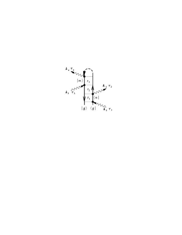
Figure 4: Each of the 12 non-time-ordered correlation function expressions for $F_{j}$ (Eq. (IV)) may be obtained from the corresponding Feynman diagram (Fig. 3) using time ordering on a Keldysh loop. This is illustrated here for $\mathbf{k}_{I}$(a). ($F_{1}(\tau_{1},\tau_{2},\tau_{4},\tau_{3})$)

Note that the absolute time arguments of $F$ in Eq. (IV) are not time ordered. However they are ordered on the Keldysh loop shown in Fig. (4) in the following sense: for each diagram we can start in the bottom right, move up on the bra line and then down on the ket line. This will give the order of the $\tau$ arguments for each of the 12 terms in Eq. (IV).

Within the slowly varying amplitude approximation the signal field is proportional to the polarization, $E_{s}(t)\propto iP_{s}^{(n)}(t)$mukbook . The simplest detection measures the time integrated signal field intensity, and the third order signal in the $\mathbf{k}_{s}$ direction is given by:

$$I_{hom}(t_{1},t_{2})=\int_{-\infty}^{+\infty}|P^{(3)}_{s}(t)|^{2}dt.$$ (28)

This is known as the homodyne detection mode. Additional time resolution may be achieved by time gating which yields the absolute value of polarization itself $I_{hom}(t_{1},t_{2},t_{3})=|P^{(3)}_{s}(t)|^{2}$.

In heterodyne detection the generated field $E_{s}(t)$ is mixed with a fourth field, ${E}_{4}(t)$ which has the same wavevector and the heretodyne signal is given by:

$$I_{het}(t_{1},t_{2},t_{3})=Im\int_{-\infty}^{+\infty}{E}_{4}^{\ast}(t)P^{(3)}_{s}(t)dt.$$ (29)

The time resolution is now determined by the heterodyne field, and the signal depends linearly rather than quadratically on $P^{(3)}_{s}(t)$. By choosing different phases of the heterodyne field it is possible to measure separately the real and the imaginary parts of the polarization.

A mixed time/frequency representation of the signal may be useful to reveal correlations in the system. For example, one can display two dimensional $\omega_{1}/\omega_{3}$ correlation plots for a fixed $t_{2}$.

$$I_{het}(\omega_{1},t_{2},\omega_{3})=\int_{0}^{+\infty}\!\!\!\int_{0}^{+\infty}dt_{1}dt_{3}I_{het}(t_{1},t_{2},t_{3})\exp(i\omega_{1}t_{1}+i\omega_{3}t_{3}).$$ (30)

Time and frequency resolved signals and fields may be displayed using the Wigner spectrogram khidekel ; ciurdariu ; schleich :

$$W_{s}(t,\omega)=\int_{-\infty}^{+\infty}E_{s}^{\ast}(t-\tau/2)E_{s}(t+\tau/2)\exp(i\omega\tau)d\tau.$$ (31)

The spectrogram directly shows what fraction of the field energy is contained in a given time and frequency window. Integrating over the frequencies gives the instantaneous field energy

$$\int_{-\infty}^{+\infty}W_{s}(t,\omega)d\omega=2\pi|E_{s}(t)|^{2}$$ (32)

while integrating over the time gives the energy density spectrum

$$\int_{-\infty}^{+\infty}W_{s}(t,\omega)dt=|\mathcal{E}_{s}(\omega)|^{2}.$$ (33)

The one dimensional projections of the spectrogram (Eqs. (32) and (33)) are known as marginals.

To express the heterodyne signal, Eqn. (29), in the Wigner representation we assume that the heterodyne field is a replica of one of the incoming fields in a nonlinear experiment, and expand the polarization to first order in this field:

$$P_{s}(t)=\int_{-\infty}^{+\infty}d\tau\tilde{S}^{(1)}(t,\tau)E_{4}(\tau).$$ (34)

$\tilde{S}$ is a non-equilibrium correlation function of the system driven by all other fields. Defining the mixed time–frequency response function

$$\tilde{S}^{(1)}(t,\omega)=\int_{-\infty}^{+\infty}\tilde{S}^{(1)}(t+\tau/2,t-\tau/2)\exp(i\omega\tau)d\tau,$$ (35)

the heterodyne signal assumes the form khidekel ; ciurdariu :

$$I_{het}(t_{1},t_{2},t_{3})=\int_{-\infty}^{+\infty}dt\int_{-\infty}^{+\infty}\frac{d\omega}{2\pi}W_{4}(t,\omega)\tilde{S}^{(1)}(t,\omega),$$ (36)

where $W_{4}(t,\omega)$ is the heterodyne spectrogram, (Eq. (31)).

Eq. (36) is exact and holds for arbitrary field envelopes. For impulsive (very short) pulses the Wigner distribution is narrowly peaked at the time of heterodyne field $\bar{\tau}_{4}$ and Eq. (36) reduces to

$$I_{het}(t_{1},t_{2},t_{3})=\tilde{S}^{(1)}(\bar{\tau}_{4},\bar{\tau}_{4})\propto Im\{E_{h}^{\ast}(\bar{\tau}_{4})P_{s}(\bar{\tau}_{4})\}.$$ (37)

In the other extreme of ideal frequency domain experiments the spectrogram is narrowly peaked around its carrier frequency $\bar{\omega}_{4}$ and

$$I_{het}(t_{1},t_{2},t_{3})=\tilde{S}^{(1)}(\bar{\omega}_{4},\bar{\omega}_{4})\propto Im\big{[}\mathcal{E}_{h}^{\ast}(\bar{\omega}_{4})P_{s}(\bar{\omega}_{4})\big{]},$$ (38)

where

$$\tilde{S}^{(1)}(\omega_{1},\omega_{2})=\int_{-\infty}^{+\infty}d\tau_{1}d\tau_{2}\tilde{S}^{(1)}(\tau_{1},\tau_{2})\exp(i\omega_{1}\tau_{1}+i\omega_{2}\tau_{2}).$$ (39)

V Pump-Probe Spectroscopy

Pump-probe is the simplest third order technique and only requires two pulses. The signal defined as the difference absorption of the probe with and without the pump is related to the polarization at $\mathbf{k}_{s}=\mathbf{k}_{1}+\mathbf{k}_{2}-\mathbf{k}_{1}$ originating from two interactions with the pump $(\omega_{1},\mathbf{k}_{1})$ and one with the probe $(\omega_{2},\mathbf{k}_{2})$. The probe serves as the heterodyne field since the signal is measured in the probe direction. This technique may thus be viewed as self-heterodyne detection. This is an incoherent technique whereby the contributions of different molecules to the signal itself (rather than to its amplitude) are additive.

We consider a sequential pump probe signal induced by short, well-separated pulses where the pump comes first, followed by the probe with a delay time of $\tau$. The signal is obtained from Eqs. (IV) and (29) by combining the $\mathbf{k}_{I}$ and $\mathbf{k}_{II}$ polarizations. We get $S_{pp}=S^{A}_{pp}+S^{B}_{pp}$, where

$$S^{A}_{pp}(\omega_{1},\omega_{2};\tau) = \int_{-\infty}^{\infty}dt\int_{0}^{\infty}dt_{3}\int_{0}^{\infty}dt_{2}\int_{0}^{\infty}dt_{1}E_{2}^{*}(t-\tau+t_{3})E_{2}(t-\tau)E_{1}^{*}(t-t_{2})E_{1}(t-t_{2}-t_{1})$$ (40)

$$\times \textrm{exp}[i\omega_{2}t_{3}+i\omega_{1}t_{1}]$$

$$\times \Big{[}F_{1}(t-t_{2}-t_{1},t-\tau+t_{3},t-\tau,t-t_{2})$$

$$+ F_{1}(t-t_{2}-t_{1},t-t_{2},t-\tau,t-\tau+t_{3})\Big{]}$$

$$+ \int_{-\infty}^{\infty}dt\int_{0}^{\infty}dt_{3}\int_{0}^{\infty}dt_{2}\int_{0}^{\infty}dt_{1}E_{2}^{*}(t-\tau+t_{3})E_{2}(t-\tau)E_{1}(t-t_{2})E_{1}^{*}(t-t_{2}-t_{1})$$

$$\times \textrm{exp}[i\omega_{2}t_{3}-i\omega_{1}t_{1}]$$

$$\times \Big{[}F_{1}(t-t_{2},t-\tau+t_{3},t-\tau,t-t_{2}-t_{1})$$

$$+ F_{1}(t-\tau,t-\tau+t_{3},t-t_{2},t-t_{2}-t_{1})\Big{]}$$

$$S^{B}_{pp}(\omega_{1},\omega_{2};\tau) = \int_{-\infty}^{\infty}dt\int_{0}^{\infty}dt_{3}\int_{0}^{\infty}dt_{2}\int_{0}^{\infty}dt_{1}\textrm{exp}[-i\omega_{2}t_{3}+i\omega_{1}t_{1}]$$ (41)

$$\times E_{2}(t+t_{3}-\tau)E_{2}^{*}(t-\tau)E_{1}^{*}(t-t_{2})E_{1}(t-t_{2}-t_{1})$$

$$\times \Big{[}F_{2}(t-t_{2}-t_{1},t-\tau+t_{3},t-\tau,t-t_{2})$$

$$+ F_{3}(t-t_{2}-t_{1},t-\tau+t_{3},t-\tau,t-t_{2})\Big{]}$$

$$+ \int_{-\infty}^{\infty}dt\int_{0}^{\infty}dt_{3}\int_{0}^{\infty}dt_{2}\int_{0}^{\infty}dt_{1}E_{2}(t+t_{3}-\tau)E_{2}^{*}(t-\tau)E_{1}(t-t_{2})E_{1}^{*}(t-t_{2}-t_{1})$$

$$\times \textrm{exp}[-i\omega_{2}t_{3}-i\omega_{1}t_{1}]$$

$$\times \Big{[}F_{2}(t-t_{2},t-\tau+t_{3},t-\tau,t-t_{2}-t_{1})$$

$$+ F_{3}(t-t_{2},t-\tau+t_{3},t-\tau,t-t_{2}-t_{1})\Big{]}$$

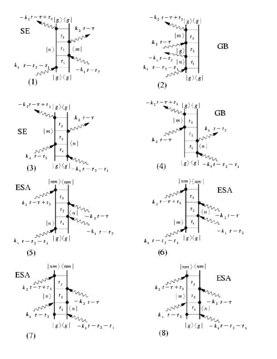
Figure 5: Feynman diagrams representing the eight contributions to the sequential pump-probe spectrum. Diagrams (1)-(8) correspond respectively to the eight terms in Eqs. (40) and (41). (1)-(4) represent the $F_{1}$ contributions (Eq. (40)), which can be divided into ground state bleaching (GB) and stimulated emission (SE) type. (5)-(8) are the $F_{2}$ and $F_{3}$ contributions (Eq. (41)), which represent excited state absorption (ESA).

These terms can be separated into two negative contributions, ground state bleaching (GB) and stimulated emission (SE) and a positive path, excited state absorption (ESA). The corresponding Feynman diagrams are shown in Fig. 5.

Using the Wigner representation (Eq. (36)), the pump probe signal can be expressed as an overlap integral of three functions: the pump spectrogram $W_{1}(t^{\prime},\omega^{\prime})$, the third order response function $S^{(3)}(t^{\prime\prime},\omega^{\prime\prime},t^{\prime},\omega^{\prime})$ and the probe spectrogram $W_{2}(t^{\prime\prime},w^{\prime\prime})$ khidekel ; ciurdariu :

$$I_{PP}(\bar{\omega}_{1},\bar{\tau}_{1},\bar{\omega}_{2},\bar{\tau}_{2},)=\int\!\!\!\int\!\!\!\int\!\!\!\int dt^{\prime}dt^{\prime\prime}d\omega^{\prime}d\omega^{\prime\prime}W_{2}(t^{\prime\prime},w^{\prime\prime})S^{(3)}(t^{\prime\prime},\omega^{\prime\prime},t^{\prime},\omega^{\prime})W_{1}(t^{\prime},\omega^{\prime}).$$ (42)

VI Fluorescence and Raman Spectroscopy

Resonant x-ray emission is widely used in the study of core-hole transitions nordgren97 ; beyondoneelectronmodel ; agrenreview99 ; nozieresandabrams ; agren01 . We consider a molecule driven by an x-ray field with a complex envelop $E(t)$ and carrier frequency $\omega_{L}$. We shall write the molecule-field interaction within the RWA in the form

$$H_{int}=E(t)B^{\dagger}\mbox{exp}\left(-i\omega_{L}t\right)+E^{*}(t)B\mbox{exp}\left(i\omega_{L}t\right).$$ (43)

$B^{\dagger}(B)$ are the exciton creation (annihilation) operators and the dipole operator is given by $\mu=$$B+B^{\dagger}$. The time and frequency resolved flourescence spectrum is given by cohentannoudjibook

$$S_{F}(\omega_{L},\omega_{S},t)=\int_{-\infty}^{\infty}d\tau\int_{-\infty}^{t}d\tau_{1}\int_{-\infty}^{t+\tau}d\tau_{2}\langle B(\tau_{2})B^{\dagger}(t+\tau)B(t)B^{\dagger}(\tau_{1})\rangle$$

$$E(\tau_{2})E^{*}(\tau_{1})\textrm{exp}\left[i\omega_{L}(\tau_{1}-\tau_{2})-i\omega_{S}\tau\right]$$ (44)

We can divide the response into time-ordered contributions which separate the Liouville space pathways into Raman and fluorescence typesmukbook . The three pathways with $\tau>0$ and $\tau<0$ are complex conjugates. This gives

$$S_{F}(\omega_{L},\omega_{S},t) = 2\textrm{Re}\int_{0}^{\infty}dt_{3}\int_{0}^{\infty}dt_{2}\int_{0}^{\infty}dt_{1}$$ (45)

$$\Big{[}E(t-t_{1}-t_{2}-t_{3})E^{*}(t-t_{2}-t_{3})\textrm{exp}(i\omega_{L}t_{1}+i\omega_{S}t_{3})F_{1}(t_{1},t_{1}+t_{2},t_{1}+t_{2}+t_{3},0)$$

$$+ E^{*}(t-t_{1}-t_{2}-t_{3})E(t-t_{2}-t_{3})\textrm{exp}(-i\omega_{L}t_{1}+i\omega_{S}t_{3})F_{1}(0,t_{1}+t_{2},t_{1}+t_{2}+t_{3},t_{1})$$

$$+ E^{*}(t-t_{1}-t_{2}-t_{3})E(t-t_{3})\textrm{exp}(-i\omega_{L}t_{1}-i(\omega_{L}-\omega_{S})t_{2}+i\omega_{S}t_{3})$$

$$\times F_{1}(0,t_{1},t_{1}+t_{2}+t_{3},t_{1}+t_{2})\Big{]}$$

The three terms in Eqn. (45) come from $R_{1}$, $R_{2}$ and $R_{3}$ respectively of Eqn. (II). It is interesting to note that $S_{F}$ only depends on $F_{1}$; four wave mixing signals also depend on $F_{2}$ and $F_{3}$, and therefore explore new regimes of Fock space not accessible by fluorescence.

We now insert the complete basis of many-body states in Eq. (III). We denote the transition frequency between states $|a\rangle$ and $|b\rangle$ as $\omega_{ab}\equiv\omega_{a}-\omega_{b}$ and $\Gamma_{ab}=\frac{1}{2}(\gamma_{a}+\gamma_{b})+\hat{\Gamma}_{ab}$ is the corresponding dephasing rate. Here $\gamma_{a}$ is the inverse lifetime of state $|a\rangle$ and $\hat{\Gamma}_{ab}$ is the pure dephasing rate resulting from frequency fluctuations. Assuming a c.w. field ($E(t)=1$), we can carry out the time integrations and obtain

$$S_{F}(\omega_{S},\omega_{L},t)=-\frac{2}{\hbar^{4}}\mbox{Re}\left(\frac{}{}S_{I}(\omega_{S},\omega_{L})+S_{II}(\omega_{S},\omega_{L})+S_{III}(\omega_{S},\omega_{L})\frac{}{}\right),$$ (46)

where

$$S_{I}(\omega_{S},\omega_{L})=-i\sum_{mn}\!\sum_{\nu_{1},\nu_{2},\nu_{3}}\!\frac{\left\langle\psi^{N}_{g}|B_{m}|\psi^{N+1}_{m,\nu_{1}}\right\rangle\left\langle\psi^{N+1}_{m,\nu_{1}}|B^{{\dagger}}_{m}|\psi^{N}_{\nu_{2}}\right\rangle\left\langle\psi^{N}_{\nu_{2}}|B_{n}|\psi^{N+1}_{n,\nu_{3}}\right\rangle\left\langle\psi^{N+1}_{n,\nu_{3}}|B^{{\dagger}}_{n}|\psi^{N}_{g}\right\rangle}{(\omega_{\nu_{1}\nu_{2}}-\omega_{S}+i\Gamma_{\nu_{1}\nu_{2}})(\omega_{\nu_{1}\nu_{3}}+i\Gamma_{\nu_{1}\nu_{3}})(\omega_{\nu_{1}g}-\omega_{L}+i\Gamma_{\nu_{1}g})}$$

$$S_{II}(\omega_{S},\omega_{L})=-i\sum_{mn}\!\sum_{\nu_{1},\nu_{2},\nu_{3}}\!\frac{\left\langle\psi^{N}_{g}|B_{m}|\psi^{N+1}_{m,\nu_{1}}\right\rangle\left\langle\psi^{N+1}_{m,\nu_{1}}|B^{{\dagger}}_{m}|\psi^{N}_{\nu_{2}}\right\rangle\left\langle\psi^{N}_{\nu_{2}}|B_{n}|\psi^{N+1}_{n,\nu_{3}}\right\rangle\left\langle\psi^{N+1}_{n,\nu_{3}}|B^{{\dagger}}_{n}|\psi^{N}_{g}\right\rangle}{(\omega_{\nu_{1}\nu_{2}}-\omega_{S}+i\Gamma_{\nu_{1}\nu_{2}})(\omega_{\nu_{1}\nu_{3}}+i\Gamma_{\nu_{1}\nu_{3}})(\omega_{L}-\omega_{\nu_{3}g}+i\Gamma_{\nu_{3}g})}$$

$$S_{III}(\omega_{S},\omega_{L})=-i\sum_{mn}\!\sum_{\nu_{1},\nu_{2},\nu_{3}}\!\frac{\left\langle\psi^{N}_{g}|B_{m}|\psi^{N+1}_{m,\nu_{1}}\right\rangle\left\langle\psi^{N+1}_{m,\nu_{1}}|B^{{\dagger}}_{m}|\psi^{N}_{\nu_{2}}\right\rangle\left\langle\psi^{N}_{\nu_{2}}|B_{n}|\psi^{N+1}_{n,\nu_{3}}\right\rangle\left\langle\psi^{N+1}_{n,\nu_{3}}|B^{{\dagger}}_{n}|\psi^{N}_{g}\right\rangle}{(\omega_{L}-\omega_{S}-\omega_{\nu_{2}g}+i\Gamma_{\nu_{2}g})(\omega_{\nu_{1}\nu_{2}}-\omega_{S}+i\Gamma_{\nu_{1}\nu_{2}})(\omega_{L}-\omega_{\nu_{3}g}+i\Gamma_{\nu_{3}g})}.$$

In the absence of dephasing, $\Gamma_{g\nu}=0,(\nu=\nu_{1},\nu_{2},\nu_{3})$, these terms can be combined to yield

$$S(\omega_{S},\omega_{L}) = \frac{2\pi}{\hbar^{4}}\sum_{\nu_{2}}\left|\sum_{n}\sum_{\nu_{1}}\frac{\left\langle\psi^{N}_{\nu_{2}}|B_{n}|\psi^{N+1}_{n,\nu_{1}}\right\rangle\left\langle\psi^{N+1}_{n,\nu_{1}}|B^{{\dagger}}_{n}|\psi^{N}_{g}\right\rangle}{\omega_{L}-\omega_{g\nu_{1}}+i\eta}\right|^{2}\delta(\omega_{L}-\omega_{S}-\omega_{g\nu_{2}})$$ (50)

where $\eta$ is an infinitesimal positive number. This is the standard expression for spontaneous emission spectramukbook .

VII The Electron-Boson Model

So far we derived exact expressions for the multipoint correlation functions in terms of the many-electron states. A much simpler description can be obtained by replacing the valence excitations by a boson bath described by the operators $a_{s}$, $a_{s}^{\dagger}$ and adding the electron-boson model Hamiltonian hedin99 ; langreth70 ; lundqvist67 ; overhauser71 ; hedin85 ; hedin98

$$H=\sum_{k}\epsilon_{k}c_{k}^{\dagger}c_{k}+\sum_{s}\omega_{s}a_{s}^{\dagger}a_{s}+\sum_{sk}V_{ks}(a_{s}+a_{s}^{\dagger})c_{k}^{\dagger}c_{k}.$$ (51)

The first two terms represent the reference Hamiltonian for the noninteracting valence and core electrons. The last term is the potential induced by the $k$’th core hole which causes a linear displacement of the bath modes.

$$U_{k}=\sum_{s}V_{ks}(a_{s}+a_{s}^{\dagger}),\qquad k=n,m$$ (52)

Each time we act with $B^{\dagger}$ we add a valence electron. If the valence system is very large (e.g. the electron gas or a large metal nanoparticle) we can ignore the effect of the additional electron and only consider the added core hole potential. In this case we can set $B^{\dagger}=c^{\dagger}$, $B=c$ and the polarization operator becomes

$$\hat{\mathbf{P}}=\sum_{k}(c_{k}+c_{k}^{\dagger}).$$ (53)

We then have

$$B_{n}^{\dagger}(\tau) = \textrm{exp}(iH_{n}\tau)\textrm{exp}(-iH_{o}\tau)$$ (54)

$$= \textrm{exp}_{-}\left[i\int_{0}^{\tau}d\tau U_{n}(\tau)\right],$$

where $H_{o}$ consists of the first two terms in Eqn. (51) so that $U_{n}\equiv H_{n}-H_{o}$ is the fluctuating potential caused by the $n$th core hole.

$$U_{n}(\tau)=\textrm{exp}(iH_{o}\tau)U_{n}\textrm{exp}(-iH_{o}\tau)$$ (55)

Similarly

$$B_{n}(\tau)=\textrm{exp}_{+}\left[-i\int_{0}^{\tau}d\tau U_{n}(\tau)\right]$$ (56)

$\textrm{exp}_{+(-)}$ refer to positive(negative) time-ordered exponentials. The multipoint correlation functions may then be calculated using the second order cumulant expansion.dariusreview ; mukpaper ; almbladh04

This is formally analogous to a multilevel molecular aggregate Hamiltonian with diagonal energy fluctuations whose nonlinear response was calculated in dariusreview ; mukpaper ; mukbook . Assuming that the transition dipole operator does not depend on the bath coordinates, we obtain

$$J(\tau)=\sum_{n}\Big{\langle}\textrm{exp}(-i\int_{0}^{\tau}d\tau_{1}U_{n}(\tau_{1})\Big{\rangle}$$ (57)

$$J(\tau)=\sum_{n}|\mu_{gn}|^{2}\exp[-i\Omega_{n}\tau-\frac{1}{2}g_{nn}(\tau)],$$ (58)

$\mathbf{\mu}_{ag}$ is the transition dipole moment between the ground state and state $a$ and $\mathbf{\mu}_{ab}$ is the transition dipole moment between excited states $a$ and $b$. The line broadening function $g_{nm}$ is associated with energy level fluctuations:

$$g_{ab}(\tau)\equiv\frac{1}{2}\int_{0}^{\tau}d\tau_{1}\int_{0}^{\tau_{1}}d\tau_{2}\,\,\left[\langle U_{a}(\tau_{1})U_{b}(\tau_{2})\rangle+\langle U_{b}(\tau_{1})U_{a}(\tau_{2})\rangle\right].$$ (59)

The four-point correlation functions may be calculated by starting with mukpaper ,

$$F_{1}(\tau_{4},\tau_{3},\tau_{2},\tau_{1}) = \sum_{n,m}\Big{\langle}\textrm{exp}_{+}\left(-i\int_{0}^{\tau_{4}}U_{m}(\tau)d\tau\right)\textrm{exp}_{-}\left(i\int_{0}^{\tau_{3}}U_{m}(\tau)d\tau\right)$$

$$\times \textrm{exp}_{+}\left(-i\int_{0}^{\tau_{2}}U_{n}(\tau)d\tau\right)\textrm{exp}_{-}\left(i\int_{0}^{\tau_{1}}U_{n}(\tau)d\tau\right)\Big{\rangle}$$

$$F_{2}(\tau_{4},\tau_{3},\tau_{2},\tau_{1}) = \sum_{n\neq m}\Big{\langle}\textrm{exp}_{+}\left(-i\int_{0}^{\tau_{4}}U_{n}(\tau)d\tau\right)\textrm{exp}_{+}\left(-i\int_{0}^{\tau_{3}}U_{m}(\tau)d\tau\right)$$

$$\times \textrm{exp}_{-}\left(i\int_{0}^{\tau_{2}}U_{m}(\tau)d\tau\right)\textrm{exp}_{-}\left(i\int_{0}^{\tau_{1}}U_{n}(\tau)d\tau\right)\Big{\rangle}$$

$$F_{3}(\tau_{4},\tau_{3},\tau_{2},\tau_{1}) = \sum_{n\neq m}\Big{\langle}\textrm{exp}_{+}\left(-i\int_{0}^{\tau_{4}}U_{m}(\tau)d\tau\right)\textrm{exp}_{+}\left(-i\int_{0}^{\tau_{3}}U_{n}(\tau)d\tau\right)$$ (60)

$$\times \textrm{exp}_{-}\left(i\int_{0}^{\tau_{2}}U_{m}(\tau)d\tau\right)\textrm{exp}_{-}\left(i\int_{0}^{\tau_{1}}U_{n}(\tau)d\tau\right)\Big{\rangle}$$

Performing the cumulant expansion to second order,ravi ; meiereee ; dariusreview we get

$$F_{1}(\tau_{4},\tau_{3},\tau_{2},\tau_{1}) = \sum_{n,m}\mu_{gm}\mu_{mg}\mu_{gn}\mu_{ng}\times$$

$$\exp[-i\Omega_{m}\tau_{43}-i\Omega_{n}\tau_{21}-f_{1}(\tau_{4},\tau_{3},\tau_{2},\tau_{1})]$$

with

$$f_{1}(\tau_{1},\tau_{2},\tau_{3},\tau_{4})= g_{nn}(\tau_{21})+g_{mm}(\tau_{43})+g_{nm}(\tau_{32})+g_{nm}(\tau_{41})-$$ (62)

$$-g_{nm}(\tau_{31})-g_{nm}(\tau_{42}).$$

$$F_{2}(\tau_{4},\tau_{3},\tau_{2},\tau_{1}) = \sum_{n\neq m}\mu_{gn}\mu_{gm}\mu_{mg}\mu_{ng}\times$$ (63)

$$\exp[-i\Omega_{m}\tau_{32}-i\Omega_{n}\tau_{41}-f_{2}(\tau_{4},\tau_{3},\tau_{2},\tau_{1})],$$

with

$$f_{2}(\tau_{1},\tau_{2},\tau_{3},\tau_{4})= g_{nn}(\tau_{41})+g_{mm}(\tau_{32})-g_{nm}(\tau_{21})$$ (64)

$$+g_{nm}(\tau_{31})-g_{mn}(\tau_{43})+g_{mn}(\tau_{42}).$$

and

$$F_{3}(\tau_{4},\tau_{3},\tau_{2},\tau_{1}) = \sum_{n\neq m}\mu_{gm}\mu_{gn}\mu_{mg}\mu_{ng}\times$$ (65)

$$\exp[-i\Omega_{m}\tau_{42}-i\Omega_{n}\tau_{31}-f_{3}(\tau_{4},\tau_{3},\tau_{2},\tau_{1})],$$

with

$$f_{3}(\tau_{4},\tau_{3},\tau_{2},\tau_{1})=g_{nn}(\tau_{31})+g_{mm}(\tau_{42})+g_{nm}(\tau_{32})-g_{nm}(\tau_{21})+g_{nm}(\tau_{41})-g_{nm}(\tau_{43}).$$ (66)

The fluctuating potentials enter the response through the spectral densities:

$${C^{\prime\prime}}_{ab}(\omega)\equiv-\frac{1}{2}\int_{-\infty}^{+\infty}dt\exp(i\omega t)\langle[U_{a}(t),U_{b}(0)]\rangle,$$ (67)

where the expectation value and the time evolution are taken with respect to the bath Hamiltonian. These contain all relevant information about the fluctuations necessary for computing the nonlinear response of the system. $g_{ab}(t)$ are directly related to the diagonal spectral densities of the bath ${C^{\prime\prime}}_{ab}(\omega)$ mukbook :

$$g_{ab}(t) = \int_{-\infty}^{\infty}\frac{d\omega}{2\pi}\frac{1-\cos(\omega t)}{\omega^{2}}\coth\left(\frac{\hbar\omega}{2k_{B}T}\right)\left[C^{{}^{\prime\prime}}_{ab}(\omega)+C^{{}^{\prime\prime}}_{ba}(\omega)\right]$$ (68)

$$+i\int_{-\infty}^{\infty}\frac{d\omega}{2\pi}\frac{\sin(\omega t)-\omega t}{\omega^{2}}\left[C^{{}^{\prime\prime}}_{ab}(\omega)+C^{{}^{\prime\prime}}_{ba}(\omega)\right]$$

These spectral densities can be obtained from photooelectron spectroscopy or inelastic x-ray scattering.schulke A simple model for the bath is given by the overdamped Brownian oscillator spectral density:mukbook

$${C^{\prime\prime}}_{ab}(\omega)=2\lambda_{ab}\frac{\omega\Lambda_{ab}}{\omega^{2}+\Lambda_{ab}^{2}}.$$ (69)

$\lambda_{aa}$ represents the magnitude of fluctuations of the energy of state $a$, while $\lambda_{ab}$ represents the fluctuation of the coupling between states $a$ and $b$. It can be observed in fluorescence as the time dependent Stokes shift. We further define the linewidth parameter $\Delta_{ab}^{2}\equiv 2k_{B}T\lambda_{ab}$. Substituting the overdamped Brownian oscillator spectral density we get in the high temperature limit:

$$g_{ab}(t)=2\left(\frac{2T\lambda_{ab}}{\Lambda_{ab}^{2}}-i\frac{\lambda_{ab}}{\Lambda_{ab}}\right)(\exp(-\Lambda_{ab}|t|)+\Lambda_{ab}t-1).$$ (70)

Two dimensionless parameters, $\eta$ and $\kappa$, can be used to characterize the model and classify different regimes of energy fluctuations. The first, $\eta$, defined by ravi $\Delta_{ab}^{2}\equiv\eta_{ab}\Delta_{aa}\Delta_{bb}$, represents the correlation of fluctuation amplitudes. $-1\leq\eta_{ab}\leq 1$. These may be anti-correlated ($\eta_{ab}=-1$), uncorrelated ($\eta_{ab}=0$) and fully correlated ($\eta_{ab}=1$). The second parameter, $\kappa_{ab}\equiv\Lambda_{ab}/\Delta_{ab}$, is the ratio of the inverse time–scale of the bath to the amplitude of the fluctuations. It controls the lineshape; in the slow bath limit ($\kappa_{ab}<1$) it has a Gaussian profile which gradually turns into a Lorentzian as $\kappa_{ab}$ is increased mukbook ; Kubo .

VIII Discussion

Nonlinear core-hole spectroscopies could provide critical tests for the limitations of the electron-boson model. Even when the core holes are localized, the valence orbitals are usually delocalized and the third order response (Eqs. (III)) requires four sets of valence orbitals corresponding to $|\psi^{N}\rangle$, $|\psi_{m}^{N+1}\rangle$, $|\psi_{n}^{N+1}\rangle$ and $|\psi_{nm}^{N+2}\rangle$. New insights could be provided on electron dynamics in conjugated molecules,mukpaper433 ; agrenreview99 and mixed valence compounds.dexheimer00 In the EBM, the effect of both core holes on the boson system is additive, (Eqn. (52)). This is why the response only depends on two collective coordinates (fluctuation potentials), $U_{n}$ and $U_{m}$. It is possible to extend this model in various ways. For example, if we add an extra coupling to Eqn. (51) $H^{\prime}=\sum_{nm}V_{nm,s}(a_{s}+a_{s}^{\dagger})c_{n}^{\dagger}c_{m}^{\dagger}c_{n}c_{m}$, the dynamics will depend on a third collective coordinate, $U_{nm}\equiv\sum_{s}V_{nm,s}(a_{s}+a_{s}^{\dagger})$. The bath displacement when both $n$ and $m$ holes exist simultaneously will then be non-additive, $U_{n}+U_{m}+U_{nm}$. The nonlinear response for this model may be calculated using the general expressions for a multilevel system given in ref (dariusreview ). Fluorescence will not depend on $U_{nm}$, since it does not affect $F_{1}$. The valence electrons generally behave as anharmonic oscillators and the Hamiltonian may contain higher order terms in $a_{s}$ and $a^{\dagger}_{s}$. Coherent nonlinear x-ray techniques may provide new information about these anharmonicities in the same way that infrared multidimensional techniques probe vibrational potential surfaces.smannreview The signal generally depends on many pulse parameters and can be displayed by various types of multidimensional correlation plots. For example, displaying the signals as a function of the time delays $t_{1}$, $t_{2}$ and $t_{3}$ provides a direct look at valence electron wavepackets. In the electron gas these probe charge density fluctuations. The third order techniques considered in this article offer numerous new probes for electron dynamics. Complementary information is provided by second order techniques such as sum and difference frequency generation.mukpaper494 These can also be analyzed using the formalism presented in the article.mukpaper512

Nonlinear core hole spectroscopy provides new ways for probing the dynamics and response of electronic valence excitations by controlled attosecond switching of external potentials. Femtosecond pulses introduced in the eighties allowed real time probing of nuclear motions. Attosecond x-ray pulses make it possible to watch electronic motions in real time. These techniques could help develop more realistic anharmonic Hamiltonians for the core-valence couplings, and test the validity of approximate model Hamiltonians.