Universality in edge-source diffusion dynamics

Abstract

We show that in edge-source diffusion dynamics the integrated concentration $N(t)$ has a universal dependence with a characteristic time-scale $\tau=({\mathcal{A}}/{\mathcal{P}})^{2}\pi/(4D)$, where $D$ is the diffusion constant while $\mathcal{A}$ and $\mathcal{P}$ are the cross-sectional area and perimeter of the domain, respectively. For the short-time dynamics we find a universal square-root asymptotic dependence $N(t)=N_{0}\sqrt{t/\tau}$ while in the long-time dynamics $N(t)$ saturates exponentially at $N_{0}$. The exponential saturation is a general feature while the associated coefficients are weakly geometry dependent.

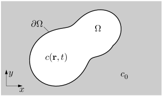
Figure 1: A sketch of the cross section $\Omega$ (white) with boundary $\partial\Omega$ (black curve) in the $xy$-pane of a rod with translational invariance in the $z$ direction. At time $t=0$, where the concentration $c(\textbf{r},t)$ inside $\Omega$ is zero, diffusion is suddenly turned on from the outside, where the concentration is kept at the constant value $c_{0}$ (gray).

Concepts like diffusion and Brownian motion are central in a wide range of complex dynamical phenomena Hänggi et al. (2005); Hänggi and Marchesonia (2005) including diffusion of ions through biological membranes, neutron diffusion in nuclear reactors, charge-carrier diffusion in semiconductors, diffusion of heat in any substance, diffusion of momentum in fluids, and diffusion of photons in the interior of the Sun Landau and Lifshitz (1987); Smith and Jensen (1989); Cussler (1997); Bird et al. (2002). In its simplest form of a scalar quantity $c$ the diffusion dynamics is governed by the linear partial differential equation

$$D\nabla^{2}c(\mathbf{r},t)=\partial_{t}c(\mathbf{r},t),$$ (1)

where $D$ is the diffusion constant. With the above notation we have emphasized diffusion of matter (with concentration $c$), but we note that the same equation also governs diffusion of energy such as in thermal problems where Eq. (1) is often referred to as the heat equation. Despite its apparent simplicity the link between space and time variables $\mathbf{r}$ and $t$ typically makes diffusion dynamics strongly dependent on the geometry and initial conditions. In this paper we find an exception to this and report a universality in edge-source diffusion dynamics. Assuming perfect translation invariance along the $z$ direction, we consider a cross section $\Omega$ in the $xy$ plane, see Fig. 1, where chemical species or heat is supplied at the boundary $\partial\Omega$. For simplicity we imagine a situation with a constant concentration $c_{0}$ outside $\Omega$ while the domain itself is empty, $c(\mathbf{r},t<0)=0$ for $\mathbf{r}\in\Omega$, before the onset of diffusion at $t=0$.

Recently, pressure-driven flow in steady-state was analyzed in the framework of simple geometrical measures Mortensen et al. (2005) such as the cross-sectional area $\mathcal{A}=\int_{\Omega}d\mathbf{r}$, the perimeter of the boundary $\mathcal{P}=\int_{\partial\Omega}d\ell$, and the compactness $\mathcal{C}=\mathcal{P}^{2}/\mathcal{A}$. In the following we study the importance of these parameters for diffusion dynamics and in particular for the integrated concentration $N(t)$ given by

$$N(t)=\int_{\Omega}d\mathbf{r}\,c(\mathbf{r},t),$$ (2)

with the limits $N(t\rightarrow 0)=0$ and $N(t\rightarrow\infty)=c_{0}\mathcal{A}$ implied by the boundary and initial conditions for $c$.

Dimensional analysis. As a first step in solving the dynamics of the integrated concentration $N(t)$ one might estimate the time-scale $\tau$ for filling up the domain. Obviously, increasing the area $\mathcal{A}$ results in an increasing filling time, while increasing the perimeter $\mathcal{P}$ or the diffusion constant $D$ results in a decreasing filling time. By dimensional analysis we thus arrive at $\tau\sim({\mathcal{A}}/{\mathcal{P}})^{2}/D$ which, as we shall see, is indeed a good estimate since detailed analysis yields

$$\tau=\left(\frac{\mathcal{A}}{\mathcal{P}}\right)^{2}\>\frac{\pi}{4D}.$$ (3)

Short-time diffusion dynamics. On a short time-scale the diffusion is perpendicular to the boundary and thus the problem is quasi-one dimensional. By a short time-scale we here mean $t\ll L_{\partial\Omega}^{2}/D$ where $L_{\partial\Omega}$ is a characteristic length scale (such as the local radius of curvature) for shape variations along the boundary $\partial\Omega$. We base our analysis on the well-known method of combination of variables originally introduced by Boltzmann Cussler (1997); Boltzmann (1894): normalization of length scales by $\sqrt{4Dt}$ reduces Eq. (1) to a 1D ordinary differential equation with the solution

$$\frac{c(\mathbf{r},t)}{c_{0}}=\textrm{erfc}\left(\frac{d_{\perp}(\mathbf{r})}{\sqrt{4Dt}}\right),$$ (4)

where $d_{\perp}(\mathbf{r})$ is the normal-distance to the boundary and $\textrm{erfc}(x)$ is the complementary error function. For $t\ll\tau$ the integrated concentration $N(t)$ becomes

$$N(t)\approx\mathcal{P}\int_{0}^{\infty}ds\,c_{0}\textrm{erfc}\Big{(}\frac{s}{\sqrt{4Dt}}\Big{)}=N_{0}\sqrt{\frac{t}{\tau}},$$ (5)

where we have introduced the characteristic time scale defined in Eq. (3) and $N_{0}=c_{0}\mathcal{A}$. The square-root dependence is a universal property for geometries with sufficiently smooth boundaries and dynamics deviating from this dependence is referred to as anomalous. Previous work on the heat content in the crushed ice model has reached results equivalent to Eq. (5) for the heat contents van den Berg and Le Gall (1994).

Table 1: The parameters $\alpha_{1}$ Eq. (9) and $\beta_{1}$ Eq. (11) for the lowest eigenfunction for differently shaped cross sections.

Cross section	$\alpha_{1}$		$\beta_{1}$
Circle	$\frac{\pi\gamma_{0,1}^{2}}{16}\simeq 1.14$		$4/\gamma_{0,1}^{2}\simeq 0.69$
Half-circle	$\frac{\pi\gamma^{2}_{1,1}}{(4+8/\pi)^{2}}\simeq 1.08$		$0.64$
Quarter-circle	$\frac{\pi\gamma^{2}_{2,1}}{(4+16/\pi)^{2}}\simeq 1.00$		$0.65$
Ellipse(1:2)	$1.18$		$0.67$
Ellipse(1:3)	$1.21$		$0.62$
Ellipse(1:4)	$1.23$		$0.58$
Triangle(1:1:1)	$\pi^{3}/36\simeq 0.86$		$6/\pi^{2}\simeq 0.61$
Triangle(1:1:$\sqrt{2}$)	$\frac{5\pi^{3}}{16(2+\sqrt{2})^{2}}\simeq 0.83$		$512/9\pi^{4}\simeq 0.58$
Square(1:1)	$\pi^{3}/32\simeq 0.97$		$64/\pi^{4}\simeq 0.66$
Rectangle(1:2)	$5\pi^{3}/144\simeq 1.08$		$64/\pi^{4}\simeq 0.66$
Rectangle(1:3)	$5\pi^{3}/128\simeq 1.21$		$64/\pi^{4}\simeq 0.66$
Rectangle(1:4)	$17\pi^{3}/400\simeq 1.32$		$64/\pi^{4}\simeq 0.66$
Rectangle(1:$\infty$)	$\sim\pi^{3}/16\simeq 1.94$		$64/\pi^{4}\simeq 0.66$
Rectangle(w:h)	$\frac{\pi^{3}}{16}\>\frac{\mathcal{C}-8}{\mathcal{C}},\mathcal{C}=\frac{4(h+w)^{2}}{hw}$		$64/\pi^{4}\simeq 0.66$
Pentagon	$1.02$		$0.67$
Hexagon	$1.05$		$0.68$

Long-time diffusion dynamics. Since $N(t)\leq N_{0}$ the result in Eq. (5) is of course only meaningful for $t\ll\tau$. When time becomes comparable to $\tau$ a saturation will occur due to decreasing gradients in density. For structures without high symmetries the saturation will be accompanied by an onset of diffusion parallel to the boundary $\partial\Omega$, and in this limit the dynamics will be slow compared to the initial behavior, Eq. (5). To study this we first derive a continuity equation by applying Green’s theorem to Eq. (1),

$$D\int_{\partial\Omega}d\ell\,\mathbf{n}\cdot\boldsymbol{\nabla}c(\mathbf{r},t)=\partial_{t}N(t).$$ (6)

Here, $\mathbf{n}$ is a normal vector to $\partial\Omega$, the integral is a line integral along $\partial\Omega$, and $-D\boldsymbol{\nabla}c$ is naturally interpreted as a current density. Next, we note that for long time-scales we have to a good approximation that $\mathbf{n}\cdot\boldsymbol{\nabla}c(\mathbf{r},t)\propto c_{0}-N(t)/\mathcal{A}$ is constant along the boundary so that

$$N_{0}-N(t)\propto\partial_{t}N(t),$$ (7)

resulting in an exponentially decaying difference. This may also be derived from an eigenfunction expansion,

$$\frac{c(\mathbf{r},t)}{c_{0}}=1-\sum_{n}f_{n}\phi_{n}(\mathbf{r})e^{-\alpha_{n}t/\tau},$$ (8)

which upon substitution into the diffusion equation yields a Helmholz eigenvalue problem for $\phi_{n}$ and $\alpha_{n}$,

$$-\nabla^{2}\phi_{n}(\mathbf{r})=\frac{4}{\pi}\left(\frac{\mathcal{P}}{\mathcal{A}}\right)^{2}\alpha_{n}\phi_{n}(\mathbf{r})$$ (9)

with $\phi_{n}(\mathbf{r})=0$ for $\mathbf{r}\in\partial\Omega$. Eq. (8) and the initial condition $c(\mathbf{r},t=0)=0$ imply that $\sum_{n}f_{n}\phi_{n}(\mathbf{r})=1$ and thus $f_{n}=\int_{\Omega}d\mathbf{r}\,\phi_{n}(\mathbf{r})/\int_{\Omega}d\mathbf{r}\,\big{|}\phi_{n}(\mathbf{r})\big{|}^{2}$. The long-time dynamics is governed by the lowest eigenvalue $\alpha_{1}$ yielding

$$\frac{N(t)}{N_{0}} =1-\sum_{n}\beta_{n}\exp\Big{(}-\alpha_{n}\frac{t}{\tau}\Big{)}$$

$$\approx 1-\beta_{1}\exp\Big{(}-\alpha_{1}\frac{t}{\tau}\Big{)},\quad t\gg\tau,$$ (10)

where

$$\beta_{n}=\frac{\mathcal{A}_{n}^{\rm eff}}{\mathcal{A}},\quad\mathcal{A}_{n}^{\rm eff}=\frac{\big{|}\int_{\Omega}d\mathbf{r}\,\phi_{n}(\mathbf{r})\big{|}^{2}}{\int_{\Omega}d\mathbf{r}\,\big{|}\phi_{n}(\mathbf{r})\big{|}^{2}}.$$ (11)

As often done in optics Mortensen (2002), $\mathcal{A}_{n}^{\rm eff}$ can be interpreted as the effective area covered by the $n$th eigenfunction. Values for a selection of geometries are tabulated in Table 1. The circle is the most compact shape and consequently it has the largest value for $\beta_{1}$, or put differently the mode has the relatively largest spatial occupation of the total area. The normalized eigenvalue $\alpha_{1}$ is of the order unity for compact shapes and in general it tends to increase slightly with increasing surface to area ratio $\mathcal{P}/\mathcal{A}$. The modest variation in both $\alpha_{1}$ and $\beta_{1}$ among the various geometries suggests that the overall dynamics of $N(t)$ will appear almost universal and that, e.g., Eq. (10) for the circle (mathematical details follow below),

$$\frac{N(t)}{N_{0}}\approx 1-\frac{4}{\gamma^{2}_{0,1}}\exp\Big{(}-\gamma^{2}_{0,1}\frac{\pi}{16}\>\frac{t}{\tau}\Big{)},\quad\gamma^{2}_{0,1}\simeq 5.783,$$ (12)

will account quantitatively well even for highly non-circular cross sections.

Analytical and numerical examples. In the following we consider a number of geometries and compare the above asymptotic expressions to analytical and numerical results. For the numerics we employ time-dependent finite-element simulations Com and solve Eq. (1) with a subsequent numerical evaluation of the integrated concentration, Eq. (2).

The circular cross section serves as a reference and an illustrative example where we directly can compare the above limits to analytical and numerical results. Applying the method of separation of variables yields Cussler (1997)

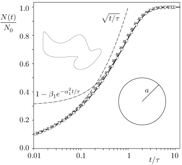
Figure 2: A lin-log plot of $N(t)/N_{0}$ as a function of $t/\tau$ for a circular cross section (white circles) and for an arbitrarily shaped cross section (gray stars); both shapes are shown in the insets. The solid line shows the exact result for the circle, i.e., the first 1000 terms in the infinite series Eq. (14), the dashed line shows the short-time asymptotic expression Eq. (5), the dot-dashed line shows the long-time asymptotic expression Eq. (12) for the circle with $\alpha_{1}=\gamma^{2}_{0,1}\pi/16$ and $\beta_{1}=4/\gamma^{2}_{0,1}$, while the data-points are the results of time-dependent finite-element simulations.

$$\frac{c_{\rm circ}(\mathbf{r},t)}{c_{0}}=1-2\sum_{n=1}^{\infty}\frac{J_{0}(\gamma_{0,n}r/a)}{\gamma_{0,n}J_{1}(\gamma_{0,n})}\>e^{-\gamma^{2}_{0,n}Dt/a^{2}},$$ (13)

where $a$ is the radius and $\gamma_{m,n}$ is the $n$th zero of the $m$th Bessel function of the first kind, $J_{m}(\gamma_{m,n})=0$. By a straightforward integration over the cross section we get

$$\frac{N_{\rm circ}(t)}{N_{0}}=1-\sum_{n=1}^{\infty}\frac{4}{\gamma^{2}_{0,n}}\>\exp\bigg{(}-\gamma^{2}_{0,n}\frac{\pi}{16}\>\frac{t}{\tau}\bigg{)},$$ (14)

where we have made the time-scale $\tau$ explicit, see Eq. (3). This result can also be derived using the continuity equation, Eq. (6). For $t>\tau$ the series converges rapidly, and keeping only the first term we arrive at Eq. (12).

In Fig. 2 we compare the asymptotic results, Eqs. (5) and (12) with the exact result, Eq. (14), as well as with time-dependent finite-element simulations. As seen both the short-time square-root and long-time exponential dependencies are in good agreement with the exact results as well as with the simulations. Fig. 2 also includes numerical results for an arbitrarily shaped cross section and, as suggested above, we see that Eqs. (5) and (12) account remarkably well even for this highly non-circular shape.

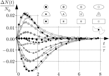
Figure 3: Plot of the deviation $\Delta N(t)/N_{0}$ from the circular case, Eq. (15), as a function of $t/\tau$ for different cross sections (see insets). The data-points are results of finite-element simulations. The ellipses have eccentricities $1,1.5,2$ and 2.5, the circle sectors have angles $\pi,2\pi/3,\pi/2$ and $\pi/3$, and the rectangles have aspect ratios $1,1.5,2$ and $3$. Note how the maximal deviation is less than $\pm 0.03$ or $\pm 3$%.

In order to see how well Eq. (14) accounts for other non-circular geometries we have employed time-dependent finite-element simulations to numerically study the relative deviations $\Delta N/N_{0}$ from it,

$$\frac{\Delta N(t)}{N_{0}}\equiv\frac{N(t)-N_{\rm circ}(t)}{N_{0}}.$$ (15)

Figure 3 summarizes results for a number of geometries. In all cases the dynamics at small times $t\ll\tau$ is in full accordance with the predicted square-root dependence, Eq. (5), and for long times the predicted exponential dependence, Eq. (12), fits the dynamics excellently. For the dynamics around $t\sim\tau$ deviations from the circular result are well within $\pm 3\%$ for the considered highly non-circular geometries.

Discussion and conclusion. We have shown that edge-source diffusion dynamics in a rod of arbitrary cross section $\Omega$ has an intrinsic time-scale $\tau=({\mathcal{A}}/{\mathcal{P}})^{2}\pi/(4D)$, with $D$ being the diffusion constant while $\mathcal{A}$ and $\mathcal{P}$ are the cross-sectional area and perimeter of $\Omega$, respectively. Initially, the filling $N(t)$ follows a universal square-root dependence $N(t)=N_{0}\sqrt{t/\tau}$, irrespectively of the shape of the domain $\Omega$. For longer times $N(t)$ saturates exponentially at $N_{0}$. The saturation is governed by the lowest dimensionless eigenvalue $\alpha_{1}$ of the Helmholz equation rather than the full spectrum. Since $\alpha_{1}$ depends only weakly on the geometry the dynamics becomes almost universal. Numerically, we have observed that the deviation from strict universality is typically less than a few percent.

Figure 4: Plots as in Fig. 3 but here for two extreme geometries: a sector of a circular disc with angle $2\arctan(1/30)$ and a rectangle with aspect ratio $1/30$, see insets. While these two shapes have nearly the same area and perimeter, the former fills slower than the circular cross section and the latter faster. The maximal deviations are $-6$% and $+10\%$, respectively.

The diffusion problem presented here relates to the question posed by Mark Kac Kac (1966): ”Can one hear the shape of a drum?”. In the present diffusion problem knowledge about the short-time dynamics allows one to extract the area to perimeter ratio $\mathcal{A}/\mathcal{P}$ while the shape itself cannot be inferred. For the long-time diffusion dynamics strict universality would require that different shapes have Helmholz eigenfunctions with the same set of eigenvalues $\big{\{}\alpha_{n}\big{\}}$ (isospectrality) and effective areas $\big{\{}\beta_{n}\big{\}}$. However, since the answer to the question of Kac in most cases is positive, see however Refs. Gordon et al. (1992); Sridhar and Kudrolli (1994), the eigenfunction properties $\big{\{}\alpha_{n}\big{\}}$ and $\big{\{}\beta_{n}\big{\}}$ of different geometries do differ. It is thus only the short-time dynamics which is strictly universal while, as mentioned above, the long-time dynamics depends weakly on shape through the first dimensionless eigenvalue $\alpha_{1}$ and the corresponding dimensionless effective area $\beta_{1}$.

Our simulations support these conclusions, see Fig. 3, and even for extreme shapes such as the narrow disc sector with angle $2\arctan(1/30)$ and the flat rectangle with aspect ratio $1/30$ the deviations from Eq. (14) are less than 10% around $t\sim\tau$, see Fig. 4. These extreme shapes have almost the same area and perimeter while the eigenfunction properties $\big{\{}\alpha_{n}\big{\}}$ and $\big{\{}\beta_{n}\big{\}}$ are very different, e.g., $\beta_{1}$ is constant $64/\pi^{4}$ for all rectangles, see Table 1, while it scales as $m^{-2/3}$ for the disc sector with angle $\pi/m$. For any aspect ratio $h/w$ the lowest eigenfunction $\phi_{1}=\sin(\pi x/w)\sin(\pi y/h)$ of the rectangle is nearly uniformly distributed in $\Omega$, and the shape favors rapid perpendicular diffusion resulting in a filling slightly faster than for the circular shape. For the disc sector with angle $\pi/m$ the lowest eigenfunction $\phi_{1}=J_{m}(\gamma_{m,1}r/a)\sin(m\theta)$ is confined to a region of width $a/m^{1/3}$ near the circular edge. This shortens the effective perimeter resulting in a filling time longer than for the circular shape. It is thus possible to find extreme shapes where $\mathcal{A}/\mathcal{P}$ is no longer the characteristic length-scale for the long-time diffusion dynamics. The same applies for a cross section with the shape of a tear drop Weisstein (1999), and for more exotic geometries, such as cross sections with a fractal polygonal boundary van den Berg and den Hollander (1999), we expect more severe deviations from the dynamics reported here. However, the deviations from strict universality obtained by extending the short-time scale $\tau$ to the long-time regime are remarkably small.

Apart from the fascinating and intriguing physics involved we believe our results are important to a number of practical problems including mass diffusion in microfluidic channels and heat diffusion in arbitrarily shaped rods.

Acknowledgements. We thank Steen Markvorsen and Ole Hansen for stimulating discussions and Michiel van den Berg for directing our attention to previous work. This work is supported by the Danish Technical Research Council (Grant Nos. 26-03-0073 and 26-03-0037).

References

- Hänggi et al. (2005) P. Hänggi, J. Luczka, and P. Talkner, New J. Phys 7 (2005), Focus on Brownian Motion and Diffusion in the 21st Century.
- Hänggi and Marchesonia (2005) P. Hänggi and F. Marchesonia, Chaos 15, 026101 (2005), Introduction: 100 years of Brownian motion.
- Landau and Lifshitz (1987) L. D. Landau and E. M. Lifshitz, Fluid Mechanics, vol. 6 of Landau and Lifshitz, Course of Theoretical Physics (Butterworth–Heinemann, Oxford, 1987), 2nd ed.
- Smith and Jensen (1989) H. Smith and H. H. Jensen, Transport Phenomena (Oxford University Press, Oxford, 1989).
- Cussler (1997) E. L. Cussler, Diffusion mass transfer in fluid systems (Cambridge University Press, Cambridge, UK, 1997), 2nd ed.
- Bird et al. (2002) R. B. Bird, W. E. Stewart, and E. N. Lightfoot, Transport Phenomena (John Wiley & Sons, New York, 2002).
- Mortensen et al. (2005) N. A. Mortensen, F. Okkels, and H. Bruus, Phys. Rev. E 71, 057301 (2005).
- Boltzmann (1894) L. Boltzmann, Wied. Ann. 53, 959 (1894).
- van den Berg and Le Gall (1994) M. van den Berg and J.-F. Le Gall, Math. Z. 215, 437 (1994).
- (10) Comsol/Femlab 3.2, www.comsol.com.
- Brack and Bhaduri (1997) M. Brack and R. K. Bhaduri, Semiclassical Physics (Addison Wesley, New York, 1997).
- Morse and Feshbach (1953) P. M. Morse and H. Feshbach, Methods of Theoretical Physics (McGraw–Hill, New York, 1953).
- Mortensen (2002) N. A. Mortensen, Opt. Express 10, 341 (2002).
- Kac (1966) M. Kac, Am. Math. Mon. 73, 1 (1966).
- Gordon et al. (1992) C. Gordon, D. L. Webb, and S. Wolpert, Bull. Amer. Math. Soc. 27, 134 (1992).
- Sridhar and Kudrolli (1994) S. Sridhar and A. Kudrolli, Phys. Rev. Lett. 72, 2175 (1994).
- Weisstein (1999) E. W. Weisstein, in MathWorld–A Wolfram Web Resource (Wolfram Research, Inc., 1999), http://mathworld.wolfram.com/TeardropCurve.html.
- van den Berg and den Hollander (1999) M. van den Berg and F. den Hollander, Proc. London Math. Soc. 78, 627 (1999).