Electronic instabilities in 3D arrays of small-diameter (3,3) carbon nanotubes
Abstract
We investigate the electronic instabilities of the small-diameter (3,3) carbon nanotubes by studying the low-energy perturbations of the normal Luttinger liquid regime. The bosonization approach is adopted to deal exactly with the interactions in the forward-scattering channels, while renormalization group methods are used to analyze the low-energy instabilities. In this respect, we take into account the competition between the effective e-e interaction mediated by phonons and the Coulomb interaction in backscattering and Umklapp channels. Moreover, we apply our analysis to relevant experimental conditions where the nanotubes are assembled into large three-dimensional arrays, which leads to an efficient screening of the Coulomb potential at small momentum-transfer. We find that the destabilization of the normal metallic behavior takes place through the onset of critical behavior in some of the two charge stiffnesses that characterize the Luttinger liquid state. From a physical point of view, this results in either a divergent compressibility or a vanishing renormalized velocity for current excitations at the point of the transition. We observe anyhow that this kind of critical behavior occurs without the development of any appreciable sign of superconducting correlations.
The development of nanoscale technology during the last decade has attracted much attention on carbon nanotubes, which are among the most promising candidates to fabricate molecular-size devices. This is mainly due to the wide variety of their electronic and transport properties, which can result in metallicmint , semiconductingsaito or even superconducting behaviorkas , depending on geometry and the way of assembling.
¿From a theoretical point of view, the confinement of electrons in the longitudinal dimension of the nanotubes induces the so-called Luttinger liquid behaviorbal ; eg ; kane ; yo ; tse . This is characterized, for instance, by the power-law dependence of the differential conductance, which has been actually observed experimentallyexp ; yao .
Such a behavior breaks down anyhow at sufficiently low temperature, and the nanotubes enter a different regime, usually driven by the quality of the contacts in the experimental setup. In particular, in the case of very transparent contacts, it has been observed that carbon nanotubes may develop superconducting correlations, inherited from superconducting electrodes (proximity effect)kas as well as intrinsic to large assemblies of massive ropessup ; priv .
The superconducting instability is anyway in competition with the so-called Peierls (or charge-density-wave) instability, which may induce a metallic-semiconducting transition caused by a lattice distorsion. The mean-field temperature of such a transition has been estimated by means of detailed calculations, and it is predicted to increase as the radius of the nanotubes becomes smallerpeierls . For tubes of typical radius, calculations find a very low (undetectable) value of , while for thinner nanotubes it is predicted to be significantly larger and competing with the superconducting critical temperature.
Nevertheless, superconductivity at about 15 K has been claimed to occur in Å-diameter nanotubestang . In the experiment reported in Ref. tang, , a strong diamagnetic behavior was interpreted as an anisotropic Meissner effect, while a genuine superconducting transition was not observed. This has opened some controversy on this issue, since ab initio simulations predict a room-temperature Peierls transition in the allowed Å-diameter geometries, namely in the (5,0)ab1 and the (3,3) nanotubesab2 . On the other hand, mean-field calculations for the (5,0) nanotubes seem to find a superconducting instability, but with a critical temperature of about 1 Kmf .
In this paper we investigate the low-energy properties of the (3,3) nanotubes by focusing on the instabilities of the Luttinger liquid behavior. We study carefully the competition between the effective e-e interaction mediated by phonons and the Coulomb repulsion. The bosonization technique is applied in order to deal exactly with the interactions in the forward-scattering channels, while renormalization group methods are used to approach the low-energy instabilities of the system, driven by the backscattering and Umklapp interactions. Moreover, we pay also special attention to the experimental conditions reported in Ref. tang, , which lead to large arrays of nanotubes embedded in a zeolite matrix. This gives rise to a large screening of the Coulomb potential, which has no counterpart in the case of single nanotubesth1 ; th2 . We study this effect by means of a generalized RPA approach, showing that the long-range intertube coupling produces an efficient screening of the intratube interactions with small momentum-transfer.
The most important result of the present study is the finding of two different low-energy phases characterized by critical (nonanalytic) behavior of the physical observables. Under the conditions corresponding to the experimental samples described in Ref. tang, , the critical behavior is related to the vanishing of one of the Luttinger liquid parameters, and it is qualitatively consistent with the large diamagnetic signal observed in Ref. tang, . We also observe that this kind of singularity occurs well before the development of any sizeable superconducting or charge-density-wave correlations in the electron system.
We start by paying attention to the interactions mediated by the Coulomb potential, which provides a strong source of repulsion between electrons in single nanotubes. In the tubular nanotube geometry, the Coulomb potential is given byeg
| (1) |
where and is the nanotube radius. The screening by the environment of external charges is in general encoded in the dielectric constant . For the sake of studying the nanotube transport properties, it is more convenient do deal with the one-dimensional (1D) projection of the potential onto the longitudinal dimension of the nanotube. This is achieved by integration of the circular coordinate, upon which we obtain the 1D Coulomb potential depending on the longitudinal momentum-transfer sar
| (2) |
is in general of the order of the inverse of the nanotube radius , as it is the memory that the 1D projection keeps of the finite transverse size.
The relative strength of the Coulomb interaction is given by the dimensionless ratio between and the Fermi velocity , which for the (3,3) nanotubes is approximately . This means that the Coloumb potential should give the dominant interaction in the forward-scattering channels, at least in single nanotubes. The processes can be classified depending on the low-energy linear branches involved in the electron-electron scatteringlouie . We recall at this point that the low-energy modes of the (3,3) nanotubes lie in a bonding and an antibonding subband that cross at two Fermi points (in the undoped system) with opposite longitudinal momentadisper . We can distinguish in particular four forward-scattering channels, labelled by their respective couplings as represented in Figs. 1 and 2. In these processes there is a nominally strong Coulomb repulsion between the electrons, as they scatter without change of their chirality and the interaction strength is simply given by the Coulomb potential (2).


The interaction channels represented in Figs. 1 and 2 are only part of the complete catalogue of scattering processes, that may be classified according to the chiralities and momentum-transfer for the interacting electronslouie . It has become usual to assign respective coupling constants to the interaction channels, in such a way that the lower index discerns whether the interacting particles shift from one Fermi point to the other , remain at different Fermi points , or they interact near the same Fermi point . The upper label follows the same rule to classify the different combinations of left-movers and right-movers, including the possibility of having Umklapp processes . As we will see, the couplings for the channels with large momentum-transfer or change of chirality of the interacting electrons have an strength which is sensibly smaller than that of the forward-scattering couplings represented in Figs. 1 and 2.
A very important point is that the system with just the forward-scattering interactions and is exactly solvable by means of bosonization techniquesemery ; sol ; gog . Thus, no matter that the Coulomb repulsion may place these interaction channels in the strong-coupling regime, the availability of an exact solution makes possible to capture the nonperturbative effects coming from the Coulomb interaction. The bosonization techniques make use of the fact that the forward-scattering interactions can be written in terms of the electron density operators corresponding to the different electron fields for the linear branches shown in Fig. 3. We adopt a notation in which the index is used to label the left- or right-moving character of the linear branch, and the index to label the Fermi point. The index stands for the two different spin projections. We may actually introduce the charge and spin density operators
| (3) | |||||
| (4) |
As long as the Coulomb interaction and the interaction mediated by exchange of phonons do not depend on the spin of the interacting electrons, we will carry out the subsequent discussion in terms of the charge density operators .

It is convenient, for instance, to introduce operators for the sum and the difference of charge densities in the bonding and the antibonding subbands of the armchair nanotubes:
| (5) | |||||
| (6) |
In terms of these operators, the hamiltonian for the forward-scattering interactions can be written in the form
| (7) | |||||
where stands again for the momentum cutoff dictated by the transverse size of the nanotube.
We observe that the symmetric and the antisymmetric combination of the charge operators in the two low-energy subbands decouple in the hamiltonian (7). This can be completely diagonalized by first introducing boson fields and (and their respective conjugate momenta, and ) defined by
| (8) | |||||
| (9) |
The hamiltoninan can be rewritten then in the form
| (10) | |||||
with renormalized velocities and charge stiffnesses given by the expressions
| (11) | |||||
| (12) |
Upon application of the canonical transformation
| , | |||||
| , | (13) |
the hamiltonian (10) becomes that of a couple of noninteracting boson fields. This picture, in which the low-energy excitations are just given by charge fluctuations (and spin fluctuations with unrenormalized velocity), is what characterizes the Luttinger liquid regime of the electron systememery ; sol . The charge stiffnesses and the renormalized velocities in the two different charge sectors dictate for instance the thermodynamic and transport properties, encoded into the compressibilities , the Drude weights and the dependence of the specific heat on the temperature sch :
| (14) | |||||
| (15) | |||||
| (16) |
The above picture will be complemented later by including the effect of the backscattering and Umklapp interactions, that tend to destabilize the Luttinger liquid regime at low temperatures. At this point, we stress that the robustness of such a regime depends on the strength of the Coulomb interaction. The consideration of the screening effects induced by the environment becomes then quite relevant, specially in the case of a large assembly of nanotubesth1 ; th2 . For the nanotube array described in Ref. tang, , the long-range Coulomb repulsion gives rise to a nonnegligible interaction between electronic currents in different nanotubes. If we label these by their respective positions and in the transverse section of the array, the intertube Coulomb potential can be expressed as
| (17) |
where denotes the longitudinal momentum-transfer. We recall that the Bessel function is logarithmically divergent in the limit . For , there is implicit a short-distance cutoff given by the radius of the nanotube, which leads then to the potential (2). The important point is that the intertube Coulomb potential gives rise to quite significant screening effects at small momentum-transfer, which modify appreciably the strength of the forward-scattering couplings described above.
In order to take into account the interaction among all the nanotubes in the array, we can adopt a generalization of the RPA scheme used in Ref. hawrylak, for the study of 2D layered sytems. In our case, the screened Coulomb potential has to satisfy the self-consistent diagrammatic equation shown in Fig. 4, with running over all the positions of the nanotubes in the array. We have then
| (18) |
where stands for the polarization of each 1D electron system. This function is known exactly at small momentum-transfersol , and here it appears multiplied by the number of subbands contributing at low-energies:
| (19) |

Equation (18) can be easily solved by introducing the Fourier transform of the Coulomb potential with respect to the nanotube position in the 2D transverse section of the array. We define for instance by
| (20) |
where stands for the nanotube separation and denotes that the integration is over the Brillouin zone for the nanotube lattice in the transverse section of the array. We define similarly as the Fourier transform of . The expression of equation (18) becomes then in momentum space
| (21) |
In what follows, we will stick to the solution of this equation at , for the sake of giving a simpler description of the screening effects in the static limit.
Within our RPA scheme, the screened Coulomb potential becomes finally
| (22) |
The most important property of is that it saturates at a finite value in the limit . This is a reflection of the fact that, for distances much larger than the nanotube separation, the array screens effectively the Coulomb interaction as a 3D system. Thus, taking a value of the bare coupling , we find that the intratube potential at vanishing momentum-transfer is (for ). This value depends slightly on the dielectric constant, as represented in Fig. 5. We will take this strength of the screened intratube Coulomb potential at as an input for the values of the forward-scattering couplings and within each nanotube in the array.

A closer look at the above analysis shows that the Coulomb potential between nearest-neighbor nanotubes also gives rise to relevant interaction channels. The new couplings needed for a consistent description of the interaction processes are catalogued in Fig. 7. They adhere to the same rules used to label the intratube couplings, but with a tilde to distinguish their intertube character. In particular, the intertube forward-scattering interactions and (preserving the chirality of the electrons within each nanotube) are affected by the screening effects described above, as they are corrected by the polarization of the different nanotubes in the array. Their strength is given by the intertube Coulomb potential, which keeps only a nonnegligible value between nearest-neighbor tubes, after screening by the nanotube array. Taking again , the intertube potential for has a value at vanishing momentum-transfer (for ). The dependence of this strength on the dielectric constant is shown in Fig. 6. Although the relative strength of the intertube forward-scattering couplings and may appear small, these are however significant as they influence the scaling of the rest of interactions at low energies, as we will see in what follows.


On the other hand, the intertube chirality-breaking interactions and give rise to a different kind of screening processes, of the type represented in Fig. 8. The effect of these processes cannot be captured in the RPA scheme described above, as the polarization with a change of chirality in the particle-hole pair diverges logarithmically at low energies. As long as the corrections depend on the 1D cutoff, they give rise instead to new screening contributions to the scaling equations for the rest of interactions. We recall that the scaling equations for the interactions of single armchair nanotubes have been obtained in Ref. louie, (up to terms quadratic in the couplings). We have found that, after incorporating the corrections from the intertube interactions, the scaling equations for the intratube couplings become
| (23) | |||||
| (24) | |||||
| (25) | |||||
| (26) | |||||
| (27) | |||||
| (28) | |||||
| (29) | |||||
| (30) | |||||
| (31) | |||||
The variable stands for minus the logarithm of the energy (temperature) scale measured in units of the high-energy cutoff of the 1D model (of the order of ). The large coefficients in front of the intertube contributions arise from the number of nearest-neighbors of each nanotube in the 3D array. Furthermore, we have also incorporated a nonperturbative improvement of the equations by writing the exact dependence of the scaling dimensions on the forward-scattering couplings, expressed in terms of the parameters.

The new intertube interactions are themselves corrected by processes that diverge logarithmically at low energy, and that give rise to respective contributions to the scaling of the intertube couplings. We can focus on the analysis of and , which have values given by the intertube potential (17) at the initial stage of the low-energy scaling. As long as this potential decays exponentially for , we can neglect the influence of other intertube interactions with momentum-transfer. The second-order diagrams that renormalize the above intertube couplings consist of particle-particle processes or particle-hole loops involving a change of chirality, as illustrated in Figs. 9 and 10. Some of the contributions depend on and . This means that these couplings have to be taken into account for a consistent description of the low-energy scaling. The complete set of scaling equations for the intertube couplings becomes:
| (32) | |||||
| (33) | |||||
| (34) | |||||
| (35) | |||||
| (36) | |||||
| (37) |

Following the flow of the scaling equations, the backscattering and Umklapp interactions are progressively enhanced as the theory is scaled down to low energies. At the initial stage of the renormalization, the values of the couplings are dictated by the Coulomb interaction and, in the case of intratube couplings, also by the effective interaction mediated by phonon-exchange. Regarding the Coulomb interaction, its contribution to forward-scattering couplings is given by the RPA calculation exposed above. Thus we have , following the trend shown in Fig. 5, while , with the potential for nearest-neighbor represented in Fig. 6. For the chirality-breaking processes, the different symmetry of ingoing and outgoing electron modes implies also a significant reduction of the Coulomb potential, as evaluated in Ref. eg, . The result is that, for the armchair (3,3) nanotubes, there is a repulsive component in the backscattering and Umklapp interactions at small momentum-transfer whose strength can be estimated as . This applies to the couplings and , as well as to the corresponding intertube couplings at small momentum-transfer. For the intratube couplings with the large momentum-transfer , the contribution by the Coulomb interaction can be obtained from the Fourier transform of the potential (1). The strength estimated in this way turns out to be .

Dealing now with the contribution from the effective phonon-mediated interaction, we note that the situation is reversed, and that the backscattering and Umklapp couplings at vanishing momentum-transfer get a smaller component than the couplings for momentum-transfer around . Previous estimates had already found that the ratio between these two different strengths is approximately 1/3 caron . More recent calculations of the phonon spectrum by means of density functional theory have led to a similar proportionab1 . More precisely, it has been found that the contributions of all the phonons with momentum-transfer add to an effective coupling , while the contributions of the phonons near the zone center give an effective coupling . These more accurate estimates are about three times smaller than those quoted in Ref. caron, . Anyhow, we will consider the phase diagram of the (3,3) nanotubes by spanning a suitable range in the scale of the two effective couplings, covering the values between the different estimates in Refs. ab1, and caron, .
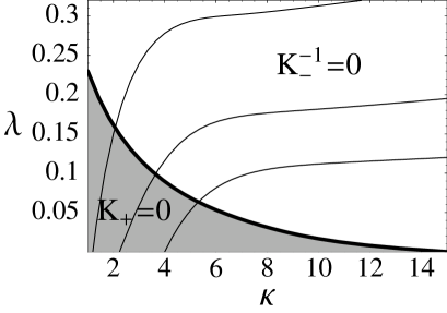
In order to determine the electronic instabilities that may appear at low energies, we have solved the set of scaling equations (23)-(37), taking initial values for the couplings according to the above discussion. The couplings approach in general a regime where they grow large as . Regarding the forward-scattering interactions, becomes increasingly repulsive, leading to a singularity characterized by either the vanishing of or the divergence of , depending on the region of the phase diagram. The scaling of the interactions stops at the low-energy scale corresponding to the point where the singularity is reached. This has actually the character of a critical point, since it gives rise to the opening of a branch cut and nonanalytic behavior in the corresponding Luttinger liquid parameter or LET . We have plotted in Fig. 11 the phase diagram of the (3,3) nanotubes showing the two different regions of singular behavior, as a function of the dielectric constant and the effective coupling of the phonon-mediated e-e interaction.
In general, the enhancement of backscattering and Umklapp interactions upon scaling may lead to a large growth of electron correlations, pointing at the tendency towards long-range order in the electron system. We have analyzed this possibility through the computation of different response functions
| (38) |
where the pair field characterizes a particular type of ordering. In the system under consideration, the most important correlation functions are found to be given by the following (Fourier transformed) fields:
where, for density wave (DW) operators, corresponds to a charge-density wave (CDW) and to a spin-density wave (SDW); while, for superconducting (SC) operators, stands for singlet superconductivity and for triplet superconductivity ( are the Pauli matrices, with ).
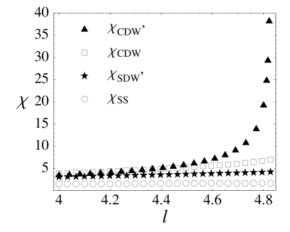
The derivatives with respect to the frequency of the response functions obey actually scaling equationssol , whose solution allows to compare the relative growth of the different electron correlations. By looking at the low-energy scaling, we have checked however that none of the response functions shows a very large growth, down to the point where the scaling flow breaks down due to the singularity in the Luttinger liquid parameter. This singular behavior occurs therefore before the appearance of any tendency to long-range order in the electron system. This is illustrated for a typical instance in Fig. 12, where it can be observed that only the CDW correlations with vanishing momentum show a significant growth as the critical point is approached.
The (3,3) carbon nanotubes may fall therefore into two different low-temperature phases, whose physical properties are dictated by the vanishing of and the divergence of respectively. We remind in particular that, for the experimental setup of Ref. tang, , a reasonable choice of the parameters is and , corresponding to the phase. In this case the temperature of transition to the new phase results strongly dependent on the dielectric constant of the environment, ranging from K (at ) to K (at ).
The behavior of the response functions follows in general the trend shown in Fig. 12 and, while the density-wave correlations tend to grow by approaching the critical value , the superconducting correlations remain small anyhow. This finding seems to rule out the possibility of having superconducting correlations in the (3,3) nanotubes, at least under the physical conditions considered in the present paper. We coincide in this respect with the conclusions reached in previous analyses by means of other computational methodsab1 ; ab2 . We have found however that the appearance of a CDW instability is precluded by the breakdown of the Luttinger liquid behavior, which cuts off the growth of the different correlations. The destabilization of the Luttinger liquid is favored in this respect by the screening effects from the 3D array of nanotubes, which are responsible of bringing the Coulomb interaction into the weak-coupling regime.
Our results confront the claim that the experimental signatures reported in Ref. tang, should provide evidence for a superconducting transition in the small-diameter nanotubes. This interpretation has been also challenged by studies of the electron correlations in the (5,0) nanotubesab1 ; nos . We have shown that, even considering the large screening effects from the arrays of nanotubes in the experimental samples, the effective e-e attraction arising from the exchange of phonons is not large enough to support the appearance of superconducting correlations in the (3,3) nanotubes. If the Coulomb interaction is further screened by a suitable variation of the dielectric constant of the medium, the system is driven then into the phase characterized by the divergence of and the related compressibility , as shown in Fig. 11. This has the same character that the instability given by the Wentzel-Bardeen singularity, where the divergent compressibility is the signal of the spatial separation of the system into regions with different electron densitylm ; dme .
Anyhow, the experimental conditions of the samples described in Ref. tang, seem to place the system in the region of the phase diagram characterized by the vanishing of . This leads to the vanishing of the conductivity at the point of the transition, as follows from Eq. (15). Moreover, it also gives rise to the vanishing of the tunneling conductance, which is directly related to the tunneling density of states . Within the Luttinger liquid framework, the latter follows the low-energy behavior
| (39) |
The depletion of the density of states given by Eq. (39) at vanishing is consistent with the appearance of the pseudogap observed experimentally in the measures of the - characteristics reported in Ref. tang, . The critical point characterized by the vanishing of does not describe however a conventional metal-insulator transition, as long as the compressibility given by Eq. (14) remains finite at the point of the transition. As analyzed in Ref. af, , the critical point implies actually a divergent diamagnetic susceptibility, as a consequence of the development of very soft modes in the sector of electron current excitations. Therefore, the phenomenology derived from the phase of the (3,3) carbon nanotubes seems to be consistent, at least qualitatively, with the main experimental signatures reported in Ref. tang, . Further experimental work would be needed to clarify the existence of such a critical point in the (3,3) nanotubes, its physical properties, and its stability under changes of relevant experimental conditions.
Acknowledgements
The financial support of the Ministerio de Educación y Ciencia (Spain) through grant BFM2003-05317 is gratefully acknowledged. E. P. was also supported by INFN grant 10068.
References
- (1) J. W. Mintmire, B. I. Dunlap and C. T. White, Phys. Rev. Lett. 68, 631 (1992).
- (2) R. Saito, M. Fujita, G. Dresselhaus and M. S. Dresselhaus, Appl. Phys. Lett. 60, 2204 (1992). N. Hamada, S. Sawada and A. Oshiyama, Phys. Rev. Lett. 68, 1579 (1992).
- (3) A. Yu. Kasumov, R. Deblock, M. Kociak, B. Reulet, H. Bouchiat, I. I. Khodos, Yu. B. Gorbatov, V. T. Volkov, C. Journet and M. Burghard, Science 284, 1508 (1999).
- (4) M. Bockrath, D. H. Cobden, J. Lu, A. G. Rinzler, R. E. Smalley, L. Balents and P. L. McEuen, Nature 397, 598 (1999).
- (5) Z. Yao, H. W. Ch. Postma, L. Balents and C. Dekker, Nature 402, 273 (1999).
- (6) L. Balents and M. P. A. Fisher, Phys. Rev. B 55, R11973 (1997).
- (7) R. Egger and A. O. Gogolin, Phys. Rev. Lett. 79, 5082 (1997); Eur. Phys. J. B 3, 281 (1998).
- (8) C. Kane, L. Balents and M. P. A. Fisher, Phys. Rev. Lett. 79, 5086 (1997).
- (9) H. Yoshioka and A. A. Odintsov, Phys. Rev. Lett. 82, 374 (1999); Phys. Rev. B 59, R10457 (1999).
- (10) A. A. Nersesyan and A. M. Tsvelik, Phys. Rev. B 68, 235419 (2003).
- (11) M. Kociak, A. Yu. Kasumov, S. Guéron, B. Reulet, I. I. Khodos, Yu. B. Gorbatov, V. T. Volkov, L. Vaccarini and H. Bouchiat, Phys. Rev. Lett. 86, 2416 (2001).
- (12) A. Kasumov, M. Kociak, M. Ferrier, R. Deblock, S. Guéron, B. Reulet, I. Khodos, O. Stéphan and H. Bouchiat, Phys. Rev. B 68, 214521 (2003).
- (13) M. T. Figge, M. Mostovoy and J. Knoester, Phys. Rev. B 65, 125416 (2002).
- (14) Z. K. Tang, L. Zhang, N. Wang, X. X. Zhang, G. H. Wen, G. D. Li, J. N. Wang, C. T. Chan and P. Sheng, Science 292, 2462 (2001).
- (15) D. Connétable, G.-M. Rignanese, J.-C. Charlier and X. Blase, Phys. Rev. Lett. 94, 015503 (2005).
- (16) K.-P. Bohnen, R. Heid, H. J. Liu and C. T. Chan, Phys. Rev. Lett. 93, 245501 (2004).
- (17) R. Barnett, E. Demler and E. Kaxiras, Phys. Rev. B 71, 035429 (2005).
- (18) J. González, Phys. Rev. Lett. 87, 136401 (2001).
- (19) J. González, Phys. Rev. Lett. 88, 076403 (2002); Phys. Rev. B 67, 014528 (2003).
- (20) D. W. Wang, A. J. Millis and S. Das Sarma, Phys. Rev. B 64, 193307 (2001).
- (21) Yu. A. Krotov, D.-H. Lee and S. G. Louie, Phys. Rev. Lett. 78, 4245 (1997).
- (22) H. J. Liu and C. T. Chan, Phys. Rev. B 66, 115416 (2002).
- (23) V. J. Emery, in Highly Conducting One-Dimensional Solids, ed. J. T. Devreese, R. P. Evrard and V. E. Van Doren (Plenum, New York, 1979).
- (24) J. Sólyom, Adv. Phys. 28, 201 (1979).
- (25) A. O. Gogolin, A. A. Nersesyan and A. M. Tsvelik, Bosonization and Strongly Correlated Systems (Cambridge Univ. Press, Cambridge, 1998).
- (26) H. J. Schulz, in Correlated Electron Systems, Vol. 9, ed. V. J. Emery (World Scientific, Singapore, 1993).
- (27) P. Hawrylak, G. Eliasson and J. J. Quinn, Phys. Rev. B 37, 10187 (1988).
- (28) A. Sédéki, L. G. Caron and C. Bourbonnais, Phys. Rev. B 65, 140515 (2002).
- (29) J. V. Alvarez and J. González, Phys. Rev. Lett. 91, 076401 (2003).
- (30) J. González and E. Perfetto, Phys. Rev. B (in press).
- (31) D. Loss and T. Martin, Phys. Rev. B 50, 12160 (1994).
- (32) A. De Martino and R. Egger, Phys. Rev. B 67, 235418 (2003).
- (33) J. González, Phys. Rev. B 72 073403 (2005).