Magnetostrictive hysteresis of TbCo/CoFe multilayers and magnetic domains.

Abstract

Magnetic and magnetostrictive hysteresis loops of TbCo/CoFe multilayers under field applied along the hard magnetization axis are studied using vectorial magnetization measurements, optical deflectometry and magneto optical Kerr microscopy. Even a very small angle misalignment between hard axis and magnetic field direction is shown to drastically change the shape of magnetization and magnetostrictive torsion hysteresis loops. Two kinds of magnetic domains are revealed during the magnetization: big regions with opposite rotation of spontaneous magnetization vector and spontaneous magnetic domains which appear in a narrow field interval and provide an inversion of this rotation.

We show that the details of the hysteresis loops of our exchange-coupled films can be described using the classical model of homogeneous magnetization rotation of single uniaxial films and the configuration of observed domains. The understanding of these features is crucial for applications (for MEMS or microactuators) which benefit from the greatly enhanced sensitivity near the point of magnetic saturation at the transverse applied field.

I Introduction

Spontaneous microscopic magnetostrictive deformations of a magnetically ordered material can be transformed into its macroscopic deformation by a modification of its magnetization structure whose energy is much lower than the energy of an equivalent elastic deformation. Materials developing this property are thus very attractive for actuator and sensor devices such as microrobots, micromotors etcClaeyssen et al. (1997),Pasquale (2003). The main advantages of magnetostrictive materials over piezoelectric or electrostrictive materials is the capability of remote addressing and controlling by an external magnetic field without direct electrical contacts.

One of the key problems for practical applications of microsystems is to reduce the magnetic driving field. The idea proposed by Quandt Quandt and Ludwig (1999),Quandt et al. (97) was to combine the giant magnetostrictive properties of rare earth transition metal based alloys (Terfenol like alloys : TbFe or TbCo) and the high magnetization and soft properties of transition metal alloys (such as CoFe) in multilayer films. In order to achieve this goal the layers should be strongly coupled. Nevertheless, even in this case it is not a priori clear whether the magnetic parameters will be a simple average of those of each individual layer or a more complex model should be used for the description of their properties.

Recent work Tiercelin et al. (2002) has shown that the well known magnetic instability of uniaxial magnetic materials in the vicinity of their saturation point under the magnetic field applied along the hard magnetization axis can be used to increase the sensitivity of micro electromechanical systems (MEMS) based on TbFe/Fe multilayers. This effect is sometimes presented as a spin reorientation phase transition at the critical field equal to the anisotropy field as was introduced in Landau and Lifchitz (1987a). At the same time the observed deformation of glass plates with TbFe/Fe multilayers deposited on them in the desired magnetic field appeared to be much more complex than expected. So, for further technical applications a better understanding of background mechanisms is necessary.

In this article we provide a detailed experimental study of magneto-elastic and magnetization behavior of multilayers with giant magnetostriction and combine them with observations of magnetic domains under the same conditions using the magneto-optical Kerr effect. The measurements are compared with a model taking into account the coherent magnetization rotation under the applied field of arbitrary direction and the role of the magnetic domains. We have selected for the demonstration our results obtained on TbCo/CoFe multilayers with very low saturation field $H_{sat}\approx 50$ Oe (4 kA/m). Our experiments on TbFe/CoFe multilayers give practically identical results.

II Experimental details

Magnetic multilayers were grown onto rectangular Corning glass substrates (22 $\times$ 5 $\times$ 0.16 mm³) from CoFe and TbCo mosaic 4 inch targets using a Z550 Leybold RF sputtering equipment with a rotary table technique. Base pressure prior to sputtering was better than $4\times 10^{-7}$ mbar. TbCo and CoFe were deposited alternatively to get a (TbCo/CoFe)₁₀ multilayer. TbCo was deposited using 150 Watt RF power and argon gas pressure of $5\times 10^{-3}$ mbar. The deposition conditions for CoFe are 200 Watt RF power and argon gas pressure of $1\times 10^{-2}$ mbar. Samples were deposited under a static field of $\sim$ 300 Oe (24 kA/m) applied along the long side of the substrate to favor an uniaxial magnetic anisotropy. No annealing treatment was applied after deposition. The sample studied in this paper is: {[Tb_34%Co_66%]60 Å/[Co_42%Fe_58%]50Å} $\times$ 10. The chemical composition was determined on separately prepared monolayer samples (TbCo and CoFe) using a X Ray Fluorescence equipment. The deposition rates were calibrated using Tencor profilometer on separate single layers. As usual for this type of material CoFe is polycrystalline while TbCo is amorphous as proved by Mössbauer spectroscopy Masson et al. (2004).

The hysteresis loops were measured using a vibrating sample magnetometer (VSM) that was modified in order to record the evolution of both longitudinal and transverse components of the sample magnetization. For this purpose two sets of detection coils either parallel to the applied field (longitudinal component $M_{L}$) or perpendicular to the applied field (transverse component$M_{T}$) were used. The vectorial measurements give direct information about the direction of the magnetization rotation crucial for the magnetoelastic behavior of the sample. The orientation $\alpha$ of the magnetic field relatively to the hard magnetization axis of the sample was varied by the rotation of the magnetometer head. Figure 1 presents a schematic diagram of the experiment.

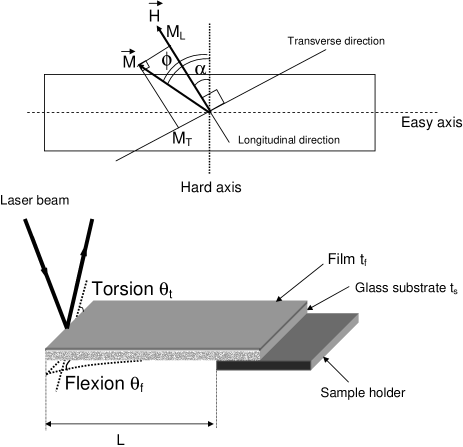
Figure 1: Geometry of the experiments: (upper panel) Magnetic measurement; (lower panel) Measurements of magnetoelastic deformations (flexion and torsion). Shown downwards flexion is defined as negative.

The magnetostrictive deformation of the samples was measured by laser deflectometry,detecting the flexion $\theta_{f}$ and torsion $\theta_{t}$ angles at the free end of the plate. The deflection of the laser beam is detected using a two dimensional position sensitive diode (PSD). The orientation of the principal axes of PSD relatively to the orientations of the laser beam displacement due to torsion and flexion was carefully adjusted. The initial angles $\theta_{f}$ and $\theta_{t}$, when there is no applied field and the magnetization is oriented along the easy axis, are taken as zero. The orientation $\alpha$ of the applied field was varied by rotation of the electromagnet independently of the optical deflectometer.

The stresses in the magnetostrictive film produce curvature of the sample with radius $R$ seen at its end as a deflection from the initial horizontal plane, $\theta_{f}=L/R$, where $L$ is the ”free” sample length. This flexion angle $\theta_{f}$, measured with field applied either parallel or perpendicular to the sample length, is used to determine the magnetoelastic coupling coefficient

$$b^{\gamma,2}=-\frac{2}{3}\frac{E_{f}}{1+\nu_{f}}\ \lambda$$

by the theory of Lacheisserie and Peuzin du Trémolet de Lacheisserie and Peuzin (1994) :

$$b^{\gamma,2}=b(H_{\parallel})-b(H_{\bot})\mbox{ at }H_{\parallel}\mbox{ and }H_{\bot}>H_{sat}\mbox{ with }$$

$$b(H_{i})=\frac{E_{s}}{6(1+\nu_{s})}\frac{\theta_{f}(H_{i})\,t_{s}^{2}}{L\,t_{f}}\quad\quad(i=\parallel,\bot)$$ (1)

The $\parallel$ and $\bot$ indexes refer to the directions of applied field: parallel or perpendicular to the sample length, which in our case coincides with the magnetic easy axis of the films (see figure 1). $\lambda$ is the magnetostriction coefficient of the film, $t_{s}$ is the substrate thickness, $t_{f}$ is the film thickness, where $t_{s}\gg t_{f}$. $E_{s}$, $E_{f}$ and $\nu_{s}$, $\nu_{f}$, are, respectively, the Young modulus and Poisson ratio of the substrate (s) and of the film (f).

For Corning glass substrates $E_{s}=60$ GPa and $\nu_{s}=0.27$. Unfortunately the elastic parameters of the film cannot be accurately determined and all techniques of magnetostriction measurements of thin films provide only $b^{\gamma,2}$, with $\lambda$ known only approximatively.

It is important to note that the equation above is valid only when the maximum vertical sample deflection is very small : $L\theta\ll t_{s}$, that is fulfilled in our experiment. In this condition the total curvature of the sample $R$ is an integral of local deformations and depends neither on its shape nor on its inhomogeneity. In this case, one can easily consider our real situation, where the principal axis of the curvature (which corresponds to the direction of sample magnetization) deviates from the sample axis. The sample has, thus, both flexion and torsion. In order to evaluate them, one can imagine a small narrow rectangle cut from a cylindrical surface of radius $R$ at an angle $\varphi$ from its axis. The rotation of the normal to the surface from one to the other end of the rectangle is $\theta_{n}=L/R\ \sin\varphi$. Its component in the direction of the sample axis is the flexion angle $\theta_{f}=\theta_{n}\sin\varphi=L/R\ \sin^{2}\varphi$, and its transversal component is the torsion angle $\theta_{t}=\theta_{n}\cos\varphi=\frac{1}{2}L/R\ \sin 2\varphi$.

When large sample deformations are required for application, the above conditions are not fulfilled and a much more complicated theory has to be used, see Guerrero and Wetherhold (2003),Wetherhold and Chopra (2001). In general, the elastic properties of thin plates are described by non-linear equations Landau and Lifchitz (1987b).

Another point to outline is that the correct definition of the positive and negative flexion angle is important for the determination of the signs of $b^{\gamma,2}$ and $\lambda$. The flexion is positive when the sample turns towards the surface covered by the magnetostrictive film (see Fig. 1). All our measurements with TbCo/CoFe and TbFe/CoFe films give negative values for $b^{\gamma,2}$ corresponding to positive $\lambda$ (elongation of the material along the applied field) as reported in the literature also for bulk TbFe and TbCo samples .

Domain observations were performed using the magneto-optical longitudinal Kerr effect (MOKE microscopy Hubert and Schäfer (1998)). The microscope is of the split-path type, with an incidence angle of 25^∘. The lenses, with a low numerical aperture ($\sim 0.1$), allow for wide field imaging of the inclined sample with good polarisation quality. The objective lens is fitted with a rotatable wave plate ($\lambda/20$) followed by a rotatable analyser, for optimal contrast adjustment. The light source is a mercury lamp with a pass-band filter around $\lambda=546$ nm. A set of coils provides field in the 3 directions. The incidence plane is parallel to the vertical side of all the images of domains presented here.

III Results and discussion

The measurements of $b^{\gamma,2}$ of our multilayers are presented in Figure 2. The fact that under the field applied along the easy direction $\theta_{f}$ remains almost constant (zero) proves the good alignment of the field.

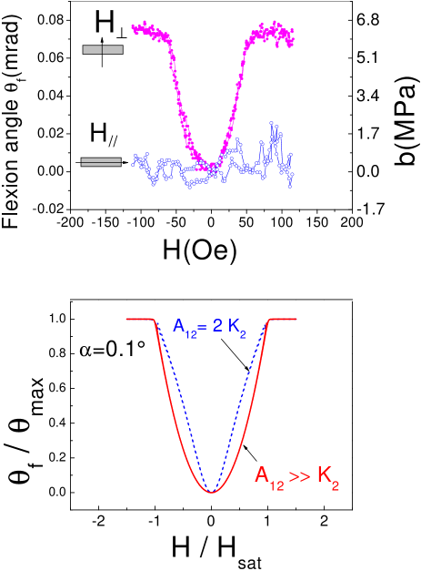
Figure 2: Flexion cycles for the field applied parallel $H_{\parallel}$ and perpendicular $H_{\bot}$ to the easy axis. Upper panel: experimental results. Lower panel: calculated torsion cycles for two cases: strongly coupled magnetizations of magnetic layers ($A_{12}\gg 2K_{2}t_{2}$, $H_{sat}=2K_{2}/\mu_{0}M_{1}t_{1}$), and moderate exchange between $M_{1}$ and $M_{2}$ ($A_{12}=4K_{2}t_{2}$, $H_{sat}\approx 4.0K_{2}t_{2}/\mu_{0}M_{1}t_{1}$)

We found a negative value of $b^{\gamma,2}\approx-7$ MPa. One should note that we have obtained an actuation field as low as 50 Oe (4 kA/m) that gives a field sensitivity much higher that reported by Betz for similar sample compositions and thicknesses Betz (1997). Our lower $b^{\gamma,2}$ is related to a lower value of Curie temperature of our samples which should be close enough to the room temperature in order to achieve maximal magnetoelastic susceptibility.

The flexion $\theta_{f}(H)$ cycle does not evolve much when the angle $\alpha$ between the hard axis and the external magnetic field is varied a few degrees around zero. Contrarily, the torsional angle loop $\theta_{t}(H)$ evolves considerably in a quite unexpected way as shown on figure 3. Not only the amplitude but also the shape of the torsional cycle change significantly when $\alpha$ is varied around zero. The characteristic ”butterfly”-like figures at small angles ($\alpha=\pm 1^{\circ}$ in Fig. 3) was already found in similar samples in Le Gall et al. (2001a) and the question of their explanation was open. Having in mind a simple monotonic magnetization rotation, one would expect a simple sinusoidal form $\theta_{t}(H)\sim\sin(H/H_{sat})$, so that the real complicated shape indicates a more complex magnetization process.

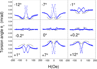
Figure 3: Experimental torsion cycles for various angles $\alpha$ between hard axis and applied field direction.

Our systematic study of the angular dependence shows that the cycles are antisymmetric around $\alpha=0$ (compare, for example, two frames in Fig. 3 corresponding to $\alpha=+12^{\circ}$ and $-12^{\circ}$): when $\alpha$ changes sign, all the figure $\theta_{t}(H)$ is reflected around the horizontal axis. On each branch of $\theta_{t}(H)$ corresponding to increasing or decreasing field wide local extrema are separated by a sharp asymmetric peak of opposite direction. It should be noted that the larger $\alpha$ is, the sharper are the central peaks. When the field is close to the hard axis ($\alpha=0$) the observed 3 torsion oscillations practically disappear. A small remaining irregular signal can be explained by a small dispersion of the orientation of the anisotropy axis throughout the sample that will be discussed further.

A more transparent interpretation of the magnetization processes behind the observed complicated magnetostrictive loops behaviour can be obtained from measurements of two components of the magnetization. Figure 4 presents the longitudinal (ordinary) $M_{L}(H)$ and transverse magnetization $M_{T}(H)$ loops obtained for different $\alpha$ angles.

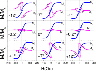
Figure 4: Experimental longitudinal ($M_{L}$) and transverse ($M_{T}$) magnetization loops for various angles $\alpha$ between hard axis and applied field direction.

The longitudinal magnetization at $\alpha=0$ has nearly no hysteresis as usual for the hard axis magnetization. At non-zero $\alpha$ some hysteresis appears. We will show below that the corresponding small coercive field is fully determined by the magnetization rotation, the coercive field of domain wall motion (corresponding to the field where the back and forth branches of the hysteresis loop merge) being higher.

The hysteresis of $M_{T}(H)$ is much more visible. The transverse loops are antisymmetric around $\alpha=0$ in a manner similar to the torsional cycles: for positive $\alpha$ when magnetic field is decreased the transverse magnetization $M_{T}$ increases first and abruptly changes from positive to negative, whereas for negative $\alpha$, $M_{T}$ first decreases and abruptly changes the sign in opposite direction. It shows clearly that the monotonic magnetization rotation, started from saturation, interrupts at some moment after the field inversion, and magnetization flips relatively to the hard axis in order to be closer to the magnetic field again. Then it continues to turn toward $\vec{H}$, now in the opposite direction. The abrupt magnetic inversion corresponds to the sharp peak on $\theta_{t}(H)$ (see Fig. 3).

We now explain the details of the magnetization rotation detected by the vectorial measurements of $M_{L}(H)$ and $M_{T}(H)$ for the case $\alpha=12^{\circ}$ (Fig. 4, see also the inset Fig. 11) using the schematic diagram of Fig. 5-(a). This behavior was first described by Stoner and Wohlfarth Stoner and E.P.Wohlfarth (1991).

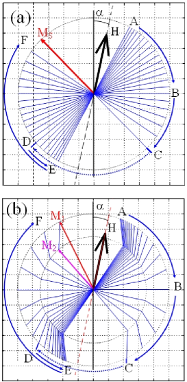
Figure 5: Vectorial diagram of the magnetization rotation in (TbFe/CoFe) multilayers. Direction of the applied field $H$ (dashed line) is deviated from hard axis by $\alpha=12^{\circ}$. In the figure easy axis is horizontal and hard axis is vertical. (a)Approximation by a single magnetization vector $\vec{M}_{s}$ (Stoner-Wohlfarth). The fan of thin lines shows the sequence of the rotation of $\vec{M}_{s}$ for field varying between $H_{max}=\frac{3}{2}H_{K}$ and $-H_{max}$ with step $\Delta H=\pm 0.1H_{K}$ ($H_{K}=\frac{2K}{\mu_{0}M_{s}}$). (b)Approximation by two coupled magnetization vectors $\vec{M}_{1}$ and $\vec{M}_{2}$ corresponding to magnetization of CoFe and TbCo layers (exchange between layers $A_{12}=4K_{2}t_{2}$).The sequence of the rotation is represented by canted lines with the point on external circle corresponding to $\vec{M}_{1}$ and the point on internal circle corresponding to $\vec{M}_{2}$. Here $H_{max}=3H_{K}(H_{K}=\frac{2K_{2}t_{2}}{\mu_{0}M_{1}t_{1}}$) and $\Delta H=\pm 0.2H_{K}$. Points A,B,..F mark characteristic moments of the magnetization rotation (see text). The vector position between points D and E superimpose for the descending and ascending field.

Let us start from the strong field $H>H_{K}$ which is applied almost perpendicularly to the easy axis and is large enough to approach the longitudinal magnetization saturation: $M_{L}\approx+M_{s}$ and $M_{T}\approx 0$ (point A in Fig. 5-(a)). When the field starts to decrease, magnetization, evidently, rotates toward the closest easy direction. $M_{L}(H)$ decreases and $M_{T}(H)$ increases continuously as can be seen (Fig. 4, $\alpha=12^{\circ}$). For $H=0$ the magnetization is aligned along the easy axis and $M_{T}\approx+M_{s}$ (point B). When the field is reversed, at some moment (point C) competition between Zeeman energy and the energy of the uniaxial magnetic anisotropy causes an abrupt magnetization switch to the opposite easy direction (point D) which becomes now closer to the field direction ($M_{T}$ changes sign). This switch is clearly visible on $M_{T}(H)$ while $M_{L}(H)$ only shows a small discontinuity which is even not visible for $\alpha=7^{\circ}$ (see Fig. 4.) After this transition the magnetization continues to rotate, now in the opposite direction, till the negative saturation: $M_{L}\approx-M_{s}$ and $M_{T}\approx 0$ again (point E). The return magnetization branch is similar but it passes ”by the other side” with $M_{T}\approx-M_{s}$ at $H=0$ (from E to F and further).

In order to describe our multilayer system more precisely we consider CoFe and TbCo layers as two interacting magnetization vectors, $\vec{M}_{1}$ and $\vec{M}_{2}$. We reduce the total energy (per surface unit) to three terms only: Zeeman energy of the CoFe layers, uniaxial magnetic anisotropy of TbCo layers and the interlayer exchange energy:

$$E(\phi_{1},\phi_{2})= - \mu_{0}M_{1}t_{1}H\cos(\phi_{1}-\alpha)-K_{2}t_{2}\sin^{2}(\phi_{2})$$ (2)

$$- A_{12}\cos(\phi_{1}-\phi_{2})$$

We neglect the Zeeman energy of the TbCo layers, because their magnetization is much smaller than that of CoFe layers, and the magnetic anisotropy energy of CoFe layers that are known as magnetically very soft. The orientations of the magnetization of both CoFe film $\phi_{1}$ and TbCo film $\phi_{2}$ are measured from the hard axis direction (see Fig. 1). $t_{1}$ and $t_{2}$ are the total CoFe and TbCo thicknesses ($t_{1}+t_{2}=t_{f}$). Magnetostrictive and elastic energies do not enter to this equation because, in our isotropic case, they do not depend on the orientation of magnetization and the curvature of the sample, due to balance of these energies that is taken into account in equation (1), remains constant. During the magnetization rotation considered here, only the orientation of the curvature changes as it was described above for the explanation of the relation of torsion and flexion.

The equilibrium angles $\phi_{1}^{\star}(H)$ and $\phi_{2}^{\star}(H)$, which correspond to local minima of $E(\phi_{1},\phi_{2})$ are numerically determined for successive values of the external field H and for its various orientations $\alpha$. Once the equilibrium angle is found, the longitudinal and transverse magnetization are simply computed since they are given principally by CoFe layers: $M_{L}=M_{1}\cos(\phi_{1}^{\star}-\alpha)$ and $M_{T}=M_{1}\sin(\phi_{1}^{\star}-\alpha)$. The flexion and torsion angles are defined by the magnetostrictive layers TbCo: $\theta_{f}=\theta_{max}\cos^{2}(\phi_{2}^{\star})$ and $\theta_{t}=\frac{1}{2}\theta_{max}\sin(2\phi_{2}^{\star})$ correspondingly (see the explanations above). Here

$$\theta_{max}=\frac{6(1+\nu_{s})}{E_{s}}\frac{L\,t_{f}}{t_{s}^{2}}b^{\gamma,2}$$

(see Eq. 1).

For sufficiently strong exchange between the layers, $A_{12}\gtrsim 2K_{2}t_{2}$, the vectors $\vec{M}_{1}$ and $\vec{M}_{2}$ turn together, the ”magnetostrictive” vector $\vec{M}_{2}$ following the leading control vector $\vec{M}_{1}$ with a delay (see the results of the numerical solution for $A_{12}=4K_{2}t_{2}$ in Fig. 5(b)). This behavior is very similar to the rotation of a single magnetization vector qualitatively described above for the classical Stoner-Wolfarth model of a simple uniaxial magnetic film (Fig. 5(a)). Both models give the characteristic points A,B,…,F with the abrupt magnetization inversion from C to D. If $A_{12}\lesssim 2K_{2}t_{2}$, this magnetization jump may disappear (depending on the value of $\alpha$).

It should be noted that CoFe and TbCo magnetizations are known to be coupled antiparallel (Betz (1997)). Nevertheless, since in our model we neglect the Zeeman energy of the TbCo layers, and since $\theta_{f}=\theta_{max}\cos^{2}(\phi_{2}^{\star})$ and $\theta_{t}=\frac{1}{2}\theta_{max}\sin(2\phi_{2}^{\star})$ the magnetization, torsion and flexion loops are not sensitive to the sign of $A_{12}$. Taking this into account, we have presented the case of positive $A_{12}$ (parallel coupling) for clarity of figure 5.

In our experimental results we do not see any effect of the delay between $\vec{M}_{1}$ and $\vec{M}_{2}$. For example, we reproduce the U-like shape of the measured flexion curve $\theta_{f}(H)$ only for $A_{12}\gg K_{2}t_{2}$ while a moderate $A_{12}$ gives a remarkably different triangular shape (Fig. 2: down panel). So, our practical multilayers can be well described by the simplest model ($A_{12}=\infty$), usually called the Stoner-Wohlfarth model, where $\vec{M}_{1}$ and $\vec{M}_{2}$ are parallel and can be, thus, represented by only one magnetization vector $\vec{M}_{s}$ (Stoner and E.P.Wohlfarth (1991),Thiaville (1998)):

$$\frac{E_{SW}(\phi)}{t_{f}}=-\mu_{0}M_{s}H\cos(\phi-\alpha)-K\sin^{2}(\phi)$$

The course of the magnetization rotation $\phi^{*}(H)$ described above (Fig. 5-(a)) was obtained by minimization of this energy for varying field between $H_{max}=\frac{3}{2}H_{k}$ and $-H_{max}$.

Figures of simulations of magnetization (Fig. 6) and magnetostriction (Fig. 7) loops are obtained from this solution using $M_{L,T}(\phi_{1}^{\star})$ and $\theta_{f,t}(\phi_{2}^{\star})$ given above with $\phi_{1}^{*}=\phi_{2}^{*}=\phi^{*}$ and $M_{1}=t_{f}/t_{1}\ M_{s}$.

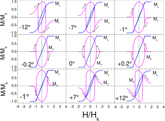
Figure 6: Longitudinal ($M_{L}$) and transverse ($M_{T}$) magnetization loops for various angles $\alpha$ between hard axis and applied field direction calculated in the framework of the model of the single magnetization vector.

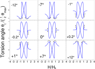
Figure 7: Torsion cycles magnetization loops for various angles ($\alpha$) between hard axis and applied field direction corresponding to the magnetization loops given in Fig. 6.

General features observed experimentally are well reproduced by this simple model. This is particularly clear for hard axis longitudinal magnetization $M_{L}(H)$ (Fig. 4 and Fig. 6, $\alpha=0$). It is linear until the saturation as for the classical case of monophase samples with good uniaxial anisotropy. In this model the anisotropy field $H_{K}$ where the extrapolation of the linear part intercepts the saturation magnetization is usually introduced. For our sample $H_{K}=\frac{2K}{\mu_{0}M_{s}}=\frac{2K_{2}t_{2}}{\mu_{0}M_{1}t_{1}}=50$ Oe (4 kA/m).

When $\alpha$ deviates from zero the longitudinal loops $M_{L}(H)$ are no longer linear and open up more and more as seen experimentally. The characteristic ”strange” butterfly shape of the torsion cycle $\theta_{t}(H)$ is also well reproduced by this model for angles $\alpha$ not too close to zero without necessity to consider more complex effects as was suggested in Le Gall et al. (2001b). The experimentally observed inversion of the ”wings” for opposite $\alpha$ follows naturally from the model as well.

When $H$ is parallel to the hard axis, two possible directions of the magnetization rotation ( clockwise or counter clockwise) and two corresponding branches of the transverse magnetization $M_{T}(H)$ (positive and negative arcs) are equivalent (Fig. 6, $\alpha=0$). The corresponding nearly zero experimental values for $M_{T}(H)$ (Fig. 4, $\alpha=0$) suggest that the sample is subdivided into magnetic domains where both opposite possibilities are realized. The magnetization in the domains alternates in a way that on average the total transverse magnetization compensates.

As soon as $\alpha$ differs from zero, one branch is favorable for the decreasing field and the opposite for the increasing field so that the experimental $M_{T}(H)$ is no longer compensated.

This remark is also valid for the torsion angle loops $\theta_{t}(H)$ (Figs. 3 and 7). For $\alpha=0$ the calculated back and forth loops are equivalent showing one minimum and one maximum. The experimental $\theta_{t}(H)$ is compensated in the same way as $M_{T}(H)$. For experimental measurements at $\alpha\neq 0$, a ”butterfly” loop opens up similarly to the calculated figures. At this moment the third additional extremum corresponding to the abrupt magnetization inversion starts to be clearly visible.

Obviously, the above model of coherent rotation (both in the simplified case of the single $\vec{M}_{s}$ vector and in the case two vectors $\vec{M}_{1}$ and $\vec{M}_{2}$) does predict the observed abrupt magnetization inversion. Nevertheless, in the experiment the transition between two magnetization ”branches” is not really abrupt: for example, at $\alpha=\pm 12^{\circ}$ the transition occurs over a field range of $\Delta H\approx 10$ Oe (800 A/m). It is well known that the abrupt coherent magnetization rotation predicted by the Stoner-Wolfarth model, at the moment when the metastable solution of $\phi^{*}$ disappears, can be realized only in small samples. In large samples the inversion from the metastable to the stable orientation is realized before reaching the instability field by means of the nucleation and motion of magnetic domains. So, in order to understand all details of the observed phenomena, one has to understand the peculiarities of the domain formation and evolution in this case.

We have directly observed the domains in our experimental situation by means of the longitudinal magneto-optical Kerr effect. The Kerr images obtained for field applied parallel to the easy axis ($\alpha=90^{\circ}$) are presented in Fig. 8. The incidence plane is also parallel to this axis. In this geometry, the observed magneto-optical contrast is proportional to the projection of $\vec{M}$ onto the easy axis. Here, and in all figures below, the image size is 3 mm $\times$ 2.2 mm. Frames a-c in Fig. 8, showing successive images obtained in decreasing field, correspond to the descending branch of the magnetization after the saturation in the positive field $H>+10$ Oe (800 A/m). At the positive saturation, all the image is dark (magnetization is directed upward). The opposite bright spontaneous magnetic domains appear at the sample edge where the stray field is maximal (at the top of the image) only when the field reverses and reaches $\sim-4$ Oe (-320 A/m). Frame (a) corresponds to the moment after the first appearance of the domains. When field sweep continues, the bright domains grow and expel the dark ones (frames (b) and (c)). The last dark domains are seen for $H=-5.1$ Oe (405 A/m). This observation corresponds well to the magnetization loop measured for $\alpha=90^{\circ}$ (see inset in Fig. 8) and its rectangular shape is usual when the field is applied along the easy magnetic direction. In this case spontaneous domains occur only in a narrow field range ($\sim$ 1 Oe (80 A/m)) where they provide the magnetization inversion. It should be noted that the domains continue to move even if the field is kept constant; this thermally activated motion gives some modification of the hysteresis loop width as function of the rate of the applied field sweep.

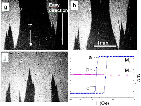
Figure 8: MOKE microscopy images for magnetic field ($H_{easy}$) applied along the easy axis following positive saturation. (a): first appearance of domains $H_{easy}=$ -4.1 Oe (325 A/m), (b): $H_{easy}=$ -4.4 Oe (350 A/m),(c): $H_{easy}=$ -4.8 Oe (380 A/m). The corresponding magnetization loop is shown in the lower-right corner. The moments where the Kerr images were obtained are marked by arrows (from a to c).

Now we pass from the classical observation of the domain motion under the field applied along the easy axis to our experiments on the hard axis magnetization. In the images below (Fig. 9) the field is applied horizontally while the incidence plane is kept in the same position (vertical). The magneto-optical contrast is proportional to the projection of $\vec{M}$ onto the vertical axis as before.

We start from the domain configuration created during the previous experiment with $\vec{H}\parallel$ easy axis (see Fig. 8). The initial domain configuration shown in Fig. 9-a is obtained after the following sequence with field applied along the easy axis: negative saturation, field inversion to $H=+4$ Oe (320 A/m) (formation of domains), $H=0$ (domain structure is frozen in). The shape of these domains does not vary when the magnetic field is applied perpendicular to the easy axis ($\alpha=0$ Fig. 9 b-c). Only the contrast between opposite domains disappears progressively corresponding to the monotonous rotation of the magnetization inside domains towards the field. The field at which the contrast becomes zero corresponds to the saturation field of the hard axis magnetization $H_{sat}=50$ Oe (4 kA/m) obtained in VSM measurements (figure 4 for $\alpha=0$).

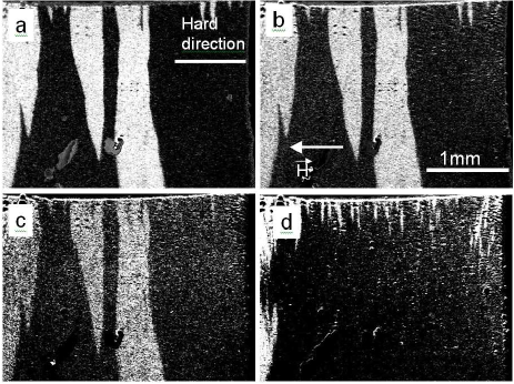
Figure 9: MOKE microscopy images for magnetic field applied along the hard direction. (a) $H=0$, the domains are prepared by an easy axis magnetization sequence (see text). Subsequent fields applied along the hard direction: (b) $H_{hard}=$30.6 Oe (2450 A/m) , (c) $H_{hard}=$44.2 Oe (3540 A/m), (d) $H=0$ after saturation at $H_{hard}>50$ Oe (4 kA/m) along the hard axis. The sample edge is visible at the top of these images.

At the saturation ($H>H_{sat}$), the image intensity is uniform (average between the dark and bright values of the initial domains). Upon the following reduction of the perpendicular field below $H_{sat}$ the initial artificially created domains never appear again. Only some very small spontaneous domains nucleate at the sample edges just below $H_{sat}$. They remain immobile until the opposite saturation just as discussed above in the case of the ”artificial” domains. Their contrast reaches a maximum at $H=0$ (Fig.9-d). It is interesting to note that the major area of the shown part of the sample became dark, i.e. the magnetization has chosen nearly everywhere here the upward easy direction. If it would be so in the whole sample, we should have observed the nice large ”butterflies” for $\theta_{t}(H)$ and arcs for $M_{T}$ which we calculated. The observed compensation of these signals means that the nearly homogeneous magnetization shown in Fig.9-d at one sample end does not extend towards its other end.

Because of an inhomogeneity of the orientation of the easy axis the different parts of the sample will have opposite orientations of the magnetization rotation towards the closest easy direction. We indeed observe a magnetic separation boundary in the central part of the sample (Fig. 10). This boundary has a complex fine structure analogous to the structure of the spontaneous domains at the sample edges and also remains immobile under the hard axis field. At zero field its magneto-optical contrast is maximal because the macrodomains separated by it have opposite magnetization along the easy axis. It should be noted that this is not a normal $180^{\circ}$ domain wall. The usual $180^{\circ}$ domain wall is nearly parallel to the easy axis and moves across the sample by the magnetic field. On the contrary, the position of the macrodomains boundary is fixed on the line where the local easy axis is parallel to the applied field. More precisely, this line is the solution of the equation $\alpha_{0}(x,y)=\alpha$ where $\alpha_{0}$ is the local orientation of the easy axis at point $x,y$ on the sample surface.

It is obvious that with a different orientation of the applied magnetic field $\alpha$, this boundary appears at a different position. In order to characterize this effect we have plotted the remanent transverse magnetization $M_{T}^{rem}$ ($M_{T}^{rem}=M_{T}(H=0$)) as a function of the angle $\alpha$ between the hard axis direction and the magnetic field (see Fig.10). For $\alpha$=0, in a homogeneous sample, one should observe $M_{T}^{rem}=\pm M_{s}$ since both rotation branches are equivalent, as discussed previously. When $\alpha$ departs from zero $\mid M_{T}^{rem}\mid$ decreases and reaches zero for $\alpha=\pm 90^{\circ}$ when the field is applied along the easy axis:

$$M_{T}^{rem}=M_{s}\,\mbox{sign}(\alpha)\,\cos(\alpha).$$

In the reality, the central step at $\alpha=0$ is smeared according to the distribution $\alpha_{0}(x,y)$ and the corresponding gradual displacement of the boundary between two opposite macro-domains with $M_{T}^{rem}=\pm M_{s}$. In our case the experimental values match the model for $|\alpha|\gtrsim 6-7^{\circ}$. This allows to quantify the easy axis distribution within the sample: its maximum deviation from the average position is about $\pm 6^{\circ}$. When the magnetic field is applied in this interval around the hard axis direction the sample is divided onto correspondingly proportioned opposite macro-domains, while when $|\alpha|>6^{\circ}$ the sample is monodomain. In our sample the observed structure of the transverse remanent magnetization corresponds to a gradual monotonous rotation of the easy axis across the sample. So, one can expect that in a smaller sample this angular range where the macro-domains appear would be narrower. It is evident, that each macro-domain represents the solutions for $M_{T}(H)$ and $\theta_{t}(H)$ shown above at positive or negative small values of $\alpha$, which have the same amplitude and shape, but change sign from one domain to another (see central frames of Figs. 6 and 7). So, the total value averaged over both domains will be compensated at $\alpha\approx 0$.

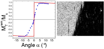
Figure 10: Characterisation of the inhomogeneity of the sample magnetic anisotropy. Left panel : dependance of the transverse remanent magnetization $M_{T}^{rem}$ of the sample on the field orientation $\alpha$. Solid circles represent the experimental masurements and solid line shows $M_{T}^{rem}(\alpha)$ expected for an ideal sample with a well defined easy axis. Right panel: MOKE image of the macrodomain boundary appeared in a central part of the sample at $H=0$ after the hard axis saturation. The magnetization here is vertical: downward in the left bright macrodomain and upward in the right dark macrodomain.

In order to illustrate the ”ideal” process of the sample magnetization at $|\alpha|>6^{\circ}$, when the magnetization rotation is homogeneous over the whole sample, we present Kerr images obtained at a field deviating by $\sim 12^{\circ}$ from the hard axis direction (Fig. 11). We see how, after the initial saturation magnetization in the negative field, the magnetization inversion starts in a positive field by nucleation of spontaneous magnetic domains at the sample edge where the stray field is maximum (Fig. 11-a). The motion of domain walls extends over a field range of some Œrsted (Fig. 11-b,c) which is considerably larger than in the case of the easy axis magnetization presented above ($\sim 10$ Oe = 800 A/m contrary to $\sim 1$ Oe =80 A/m) but remains rather narrow in comparison with the overall width of the hysteresis ($H_{d}\sim 30$ Oe = 2400 A/m) as seen in the hysteresis loops presented in the inset.

It is important to note here the difference between the transverse hysteresis width ($H_{d}$, the field at which the magnetization vector flips from one side to the other, i.e. $M_{T}(H_{d})=0$) and the usual coercive field ($H_{c}$, where $M_{L}(H_{c})=0$). $H_{d}(\alpha)$ represents the coercive field of the domain wall motion reached when the corresponding force is equilibrated by the difference of the Zeeman energy density : $F_{C}(\vec{M}_{+},\vec{M}_{-})=\vec{H_{d}}\cdot(\vec{M}_{+}-\vec{M}_{-})$. Here $\vec{M}_{+}$, $\vec{M}_{-}$ are magnetizations of domains with opposite transversal components.

For $\alpha\sim 0$, $H_{d}$ becomes as large as the saturation field $H_{K}$ and the domains remain immobile between $\pm H_{d}$ as demonstrated in Fig. 9. $H_{d}\equiv H_{c}$ only for large deviation from the hard axis. For sufficiently small $\alpha$ the magnetization ”jump” on the magnetization hysteresis curve $M_{L}(H)$ (the short interval of the domain motion) appears after it crosses the horizontal axis. So, $H_{c}$ has nothing to do with the domain wall motion and does not correspond to any discontinuity of the magnetization process. In this case (for example for $\alpha=12^{\circ}$, Fig. 11), $H_{c}$ represents the hysteresis of the homogeneous magnetization rotation. Obviously for $\alpha=0$, $H_{c}=0$.

It is interesting that the coherent magnetization rotation dominates the major part of the hysteresis even for so big samples, where normally the magnetization by domains is considered as the most important. These features were already observed in the case of simple monolayer films by Prutton Prutton (1964) and in spin-valve multilayers Labrune et al. (1997). The model of the coherent magnetization rotation explains the experiments so well because, when the pinning of the domain walls is sufficiently strong, or the domain wall nucleation sufficiently difficult, the domains appear and move just before the moment of the rotational instability. The resulting behavior does not differ very much from the calculated abrupt magnetization inversion.

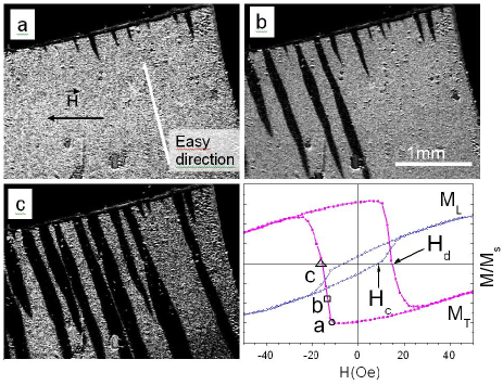
Figure 11: MOKE microscopy images for magnetic field deviating by 12^∘ from the hard axis. (a) $H=-10.5$ Oe (845 A/m). (b) $H=-12.9$ Oe (1030 A/m). (c) $H=-14.6$ Oe (1170 A/m) in sequence after saturation in positive field. These points are indicated on the corresponding measured magnetization loop $M_{T}(H)$ (central part) shown in the lower-right panel together with the ”standard” $M_{L}(H)$. The illustrated magnetization inversion corresponds to the jump $C\rightarrow D$ in Fig. 5 realized by motion of domains.

Very few investigations of domains in magnetostrictive multilayers are known. Chopra and co-workers Chopra et al. (1999) showed that in their demagnetized state individual layer of as deposited TbFe/CoFe are single domain due to stray field coupling between adjacent layers. Our measurements and direct observations, on the contrary, show that all layers are connected together by magnetic exchange and the magnetization in the whole stack of the layers turns as a single magnetic vector. The magnetic domains which inevitably appear in our sample are the same in all layers (the magneto-optical contrast is always homogeneous) and the domain walls go through the whole film.

Recently Shull and coworkers Shull et al. (2004) studied the influence of stress on domain wall structure in similar multilayers using the magneto-optic indicator film (MOIF) technique that reveals domains by an indirect effect of their stray field. They show that magnetization reversibly rotates when stress is applied whereas magnetization rotation under field application is irreversible and includes wall motion. This work of Shull et al. is limited only to easy axis magnetization when there is no magnetostrictive deformation of the sample. We show that in the practically important geometry of the hard axis magnetization, when the magnetostrictive deformation is maximal, the magnetization rotation is dominating. Our observations via the direct magneto-optical contrast give a more clear image of domains and the magnetization distribution inside them. Studies of the influence of the applied stresses on the domain structure and motion of the domain walls in TbCo/CoFe multilayers will be published elsewhere.

IV Conclusion

As result of the systematic angular measurements of all components of magnetization and magnetostrictive deformation together with a simple model, the magnetization process of magnetostrictive TbCo/CoFe multilayer has been fully understood. We have shown that even in large (centimeter size) samples the major part of the magnetic hysteresis is related to a coherent magnetization rotation inside domains. The coherent magnetic rotation is broken only once when a rather abrupt magnetization reversal occurs with appearance of spontaneous magnetic domains. In addition, we have revealed the appearance of stationary macro-domains related to the sample inhomogeneity: They explain the disappearance of the torsion angle loop and transverse magnetization when magnetic field is applied along the hard axis. A small misalignment of magnetic field modifies noticeably these loops as the ratio of opposite macro-domains changes. The appearance of the micro- and macro-domains in this system and the related effects should be taken into account in further development of technical applications of the magnetostrictive films. This is particularly important for the reduction of the lateral size of the micro-actuators.