Enhanced Conductance Through Side-Coupled Double Quantum Dots

Abstract

Conductance, on-site and inter-site charge fluctuations and spin correlations in the system of two side-coupled quantum dots are calculated using the Wilson’s numerical renormalization group (NRG) technique. We also show spectral density calculated using the density-matrix NRG, which for some parameter ranges remedies inconsistencies of the conventional approach. By changing the gate voltage and the inter-dot tunneling rate, the system can be tuned to a non-conducting spin-singlet state, the usual Kondo regime with odd number of electrons occupying the dots, the two-stage Kondo regime with two electrons, or a valence-fluctuating state associated with a Fano resonance. Analytical expressions for the width of the Kondo regime and the Kondo temperature are given. We also study the effect of unequal gate voltages and the stability of the two-stage Kondo effect with respect to such perturbations.

I Introduction

The advances in micro-fabrication have enabled studies of transport through single as well as coupled quantum dots, where at very low temperatures Kondo physics and magnetic interactions play an important role. A double-dot system represents the simplest possible generalization of a single-dot system which has been extensively studied in the past. Recent experiments demonstrate that an extraordinary control over the physical properties of double dots can be achieved Jeong et al. (2001); Craig et al. (2004); Holleitner et al. (2002); Chen et al. (2004), which enables direct experimental investigations of the competition between the Kondo effect and the exchange interaction between localized moments on the dots. One manifestation of this competition is a two stage Kondo effect that has recently been predicted in multilevel quantum dot systems with explicit exchange interaction coupled to one or two conduction channels Hofstetter and Schoeller (2003); Hofstetter and Zarand (2004). Experimentally, it manifests itself as a sharp drop in the conductance vs. gate voltage $G(V_{G})$ van der Wiel et al. (2002) or as non-monotonic dependence of the differential conductance vs. drain-source voltage $dI/dV_{ds}(V_{ds})$ Granger et al. (2005).

Fano resonances, which occur due to interference when a discrete level is weakly coupled to a continuous band, were recently observed in experiments on rings with embedded quantum dots Kobayashi et al. (2002) and quantum wires with side-coupled dots Kobayashi et al. (2004). The interplay between Fano and Kondo resonance was investigated using equation of motion Bulka and Stefanski (2001); Stefanski et al. (2004) and slave boson techniques Lara et al. .

In this work we study a double quantum dot (DQD) in a side-coupled configuration (Fig. 1), connected to a single conduction-electron channel. Systems of this type were studied previously using non-crossing approximation Kim and Hershfield (2001), embedding technique Apel et al. (2004) and slave-boson mean field theory Kang et al. (2001); Lara et al. . Numerical renormalization group (NRG) calculations were also performed recently Cornaglia and Grempel (2005), where only narrow regimes of enhanced conductance were found at low temperatures. We will show that when the intra-dot overlap is large, wide regimes of enhanced conductance as a function of gate-voltage exist at low temperatures due to the Kondo effect, separated by regimes where localized spins on DQD are antiferromagnetically (AFM) coupled. Kondo temperatures $T_{K}$ follow a prediction based on Schrieffer-Wolff transformation and poor-man’s scaling. In the limit when the dot $a$ is only weakly coupled, the system enters the ”two stage” Kondo regime Vojta et al. (2002); Cornaglia and Grempel (2005), where we again find a wide regime of enhanced conductivity under the condition that the high- and the low- Kondo temperatures ($T_{K}$ and $T_{K}^{0}$ respectively) are well separated and the temperature of the system $T$ is in the interval $T_{K}^{0}\ll T\ll T_{K}$.

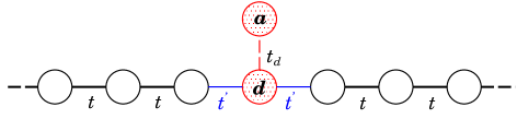
Figure 1: Side-coupled configuration of quantum dots

II Model and method

The Hamiltonian that we study reads

$$\begin{split}H&=\delta_{d}(n_{d}-1)+\delta_{a}(n_{a}-1)-t_{d}\sum_{\sigma}\left(d^{\dagger}_{\sigma}a_{\sigma}+a^{\dagger}_{\sigma}d_{\sigma}\right)\\ &+\frac{U_{d}}{2}(n_{d}-1)^{2}+\frac{U_{a}}{2}(n_{a}-1)^{2}\\ &+\sum_{k\sigma}\epsilon_{k}c^{\dagger}_{k\sigma}c_{k\sigma}+\sum_{k\sigma}V_{d}(k)\left(c^{\dagger}_{k\sigma}d_{\sigma}+d^{\dagger}_{\sigma}c_{k\sigma}\right),\end{split}$$ (1)

where $n_{d}=\sum_{\sigma}d^{\dagger}_{\sigma}d_{\sigma}$ and $n_{a}=\sum_{\sigma}a^{\dagger}_{\sigma}a_{\sigma}$. Operators $d^{\dagger}_{\sigma}$ and $a^{\dagger}_{\sigma}$ are creation operators for an electron with spin $\sigma$ on site $d$ or $a$. On-site energies of the dots are defined by $\epsilon=\delta-U/2$. For simplicity, we choose the on-site energies and Coulomb interactions to be equal on both dots, $\delta_{a}=\delta_{d}=\delta$ and $U_{a}=U_{d}=U$. Coupling between the dots is described by the inter-dot tunnel coupling $t_{d}$. Dot $d$ couples to both leads with equal hopping $t^{\prime}$. As it couples only to symmetric combinations of the states from the left and the right lead, we have used a unitary transformation Glazman and Raikh (1988) to describe the system as a variety of the single-channel, two-impurity Anderson model. Operator $c_{k\sigma}^{\dagger}$ creates a conduction band electron with momentum $k$, spin $\sigma$ and energy $\epsilon_{k}=-D\cos{k}$, where $D=2t$ is the half-bandwidth. The momentum-dependent hybridization function is $V_{d}(k)=-(2/\sqrt{N+1})\,t^{\prime}\sin{k}$, where $N$ in the normalization factor is the number of conduction band states.

We use Meir-Wingreen’s formula for conductance in the case of proportionate coupling Meir and Wingreen (1992) which is known to apply under very general conditions (for example, the system need not be in a Fermi-liquid ground state) with spectral functions obtained using the NRG technique Wilson (1975); Costi (2001); Krishna-Murthy et al. (1980); Hofstetter (2000). At zero temperature, the conductance is

$$G=G_{0}\pi\Gamma\rho_{d}(0),$$ (2)

where $G_{0}=2e^{2}/h$, $\rho_{d}(\omega)$ is the local density of states of electrons on site $d$ and $\Gamma/D=(t^{\prime}/t)^{2}$.

The NRG technique consists of logarithmic discretization of the conduction band, mapping onto a one-dimensional chain with exponentially decreasing hopping constants, and iterative diagonalization of the resulting Hamiltonian Wilson (1975). Only low-energy part of the spectrum is kept after each iteration step; in our calculations we kept 1200 states, not counting spin degeneracies, using discretization parameter $\Lambda=1.5$.

III Strong inter-dot coupling

III.1 Conductance and correlation functions

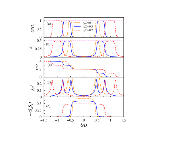
Figure 2: Conductance and correlation functions of DQD vs. $\delta$. Besides different values of $t_{d}$, indicated in the figure, other parameters of the model are $\Gamma/D=0.03$ and $U/D=1$. Temperature is $T/D=10^{-9}$, which for all parameters used corresponds to a zero temperature limit. In particular, in the Kondo plateaux $T\ll T_{K}$ for all $\delta$.

In Fig. 2a we present conductance through a double quantum dot at different values of intra-dot couplings vs. $\delta$. Due to formation of Kondo correlations, conductance is enhanced, reaching the unitary limit in a wide range of $\delta$.

To better understand multidot problems in the case of strong inter-dot coupling, it is helpful to exactly diagonalize the part of the Hamiltonian that describes the dots and rewrite the entire Hamiltonian (Eq. 1) in a form similar to the ionic model Hewson (1993):

$$H_{0}=\sum_{k,\sigma}\epsilon_{k}c^{\dagger}_{k,\sigma}c_{k,\sigma}+\sum_{\alpha}E(\alpha)|\alpha\rangle\langle\alpha|$$ (3)

$$H_{1}=\sum_{k,\sigma,\alpha,\beta}t_{k\sigma|\beta\to\alpha}\ |\alpha\rangle\langle\beta|\ c_{k,\sigma}+t^{*}_{k\sigma|\beta\to\alpha}c^{\dagger}_{k\sigma}\ |\beta\rangle\langle\alpha|.$$ (4)

where multi-indeces $\alpha$ and $\beta$ stand for quantum numbers $(Q,S,S_{z},r)$. Here $Q$ is the charge number $Q=(n_{a}-1)+(n_{d}-1)$, $S,S_{z}$ are the spin and its component, while $r$ numbers different states with the same $Q,S,S_{z}$ quantum numbers. In the absence of the magnetic field, $S_{z}$ is irrelevant and will be omitted from now on. Each $(Q,S,r)$ multiplet is then $2S+1$-fold degenerate. Finally, the effective hopping coefficients

$$t_{k\sigma|\beta\to\alpha}=V_{d}(k)\langle\alpha|d_{\sigma}^{\dagger}|\beta\rangle$$ (5)

correspond to electrons hopping from the conduction band to the dots.

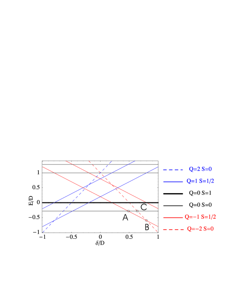
Figure 3: Eigenvalue diagram for isolated DQD system. The diagram is symmetric, since for $\delta\to-\delta$, $E(Q,S,r)\to E(-Q,S,r)$. Points $A$ and $B$ correspond to valence-fluctuation regions when the charge on the dot changes, while point $C$ corresponds to the center of the Kondo regime, when the Kondo temperature is the lowest. Parameters are $U/D=1$ and $t_{d}/D=0.3$.

The eigenvalue diagram in Fig. 3 represents the gate-voltage dependence of the multiplet energies $E(Q,S,r)$. From this diagram we can read off the ground state and the excited states for each parameter $\delta$.

Regimes of enhanced conductance appear in the intervals approximately given by $\delta_{1}<|\delta|<\delta_{2}$, where $\delta_{1}=t_{d}(2\sqrt{1+(U/4t_{d})^{2}}-1)$ and $\delta_{2}=(U/2+t_{d})$. These estimates are obtained from the lowest energies of states with zero, one and two electrons on the isolated double quantum dot:

$$\begin{split}E(-2,0,0)&=U-2\delta,\\ E(-1,\tfrac{1}{2},0)&=U/2-\delta-t_{d},\\ E(0,0,0)&=-2t_{d}\sqrt{1+(U/4t_{d})^{2}}+U/2.\end{split}$$ (6)

The widths of conductance peaks (measured at $G/G_{0}=1/2$) are therefore approximately given by

$$\Delta=U/2+2t_{d}(1-\sqrt{1+(U/4t_{d})^{2}}).$$ (7)

Note that in the limit of large $t_{d}$, $\Delta\simeq U/2$, and in the limit of large $U$, $\Delta\simeq 2t_{d}$. As it will become apparent later in this paper, this naive estimate fails when $t_{d}\to 0$. Comparison of conductance-peak widths with the analytical estimate $\Delta$ is shown in Fig. 4a.

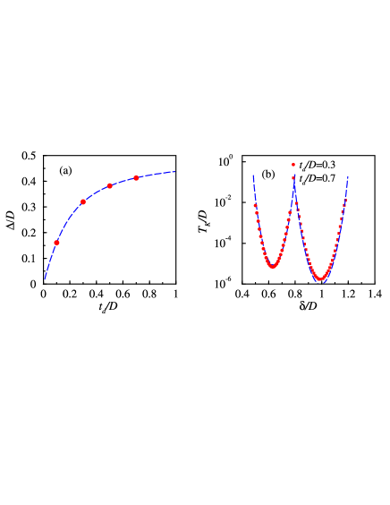
Figure 4: a) The width of conductance peak $\Delta$ vs. $t_{d}$ as obtained from NRG calculations (full circles), compared with the analytical result as given in the text (dashed line). b) Kondo temperatures $T_{K}$ vs. $\delta$ as obtained from the widths of Kondo peaks (full circles). Analytical estimate, Eq. 8, is shown using dashed lines. The rest of parameters are identical to those in Fig. 2.

Next, we focus on various correlation functions. In Fig. 2b we show $S$, calculated from expectation value $\langle{\bf S}_{\mathrm{tot}}^{2}\rangle=S(S+1)$, where ${\bf S}_{\mathrm{tot}}={\bf S}_{a}+{\bf S}_{d}$ is the total spin operator. $S$ reaches value $1/2$ in the regime where $G/G_{0}=1$. Enhanced conductance is thus followed by the local moment formation, indicative of the Kondo effect. This is further supported by the average double-dot occupancy $\langle n\rangle$, where $n=n_{a}+n_{d}$, which in the regime of enhanced conductivity approaches odd-integer values, i.e. $\langle n\rangle=1$ and $3$ (see Fig. 2c). Transitions between regimes of nearly integer occupancies are rather sharp; they are visible as regions of enhanced charge fluctuations measured by $\Delta n^{2}=\langle n^{2}\rangle-\langle n\rangle^{2}$, as shown in Fig. 2d. Finally, we show in Fig. 2e spin-spin correlation function $\langle{\bf S}_{a}\cdot{\bf S}_{d}\rangle$. Its value is negative between two separated Kondo regimes where conductance approaches zero, i.e. for $-\delta_{1}<\delta<\delta_{1}$, otherwise it is zero. This regime further coincides with $\langle n\rangle\sim 2$. Each dot thus becomes nearly singly occupied and spins on the two dots form a local singlet due to effective exchange coupling $J_{\mathrm{eff}}\approx 4t_{d}^{2}/U$. Surprisingly, the absolute value of $\langle{{\bf S}_{a}\cdot{\bf S}_{d}}\rangle$ increases and it nearly reaches its limiting value, i.e. $\langle{\bf S}_{a}\cdot{\bf S}_{d}\rangle=-3/4$, as the intra-dot hopping $t_{d}$, and with it $J_{\mathrm{eff}}$, decrease. This seeming contradiction is resolved by recognizing that $J_{\mathrm{eff}}$ represents the exchange interaction based on the effective Heisenberg coupling between localized spins on DQD only in the limit when $t_{d}/U\to 0$. Smaller absolute values of $\langle{{\bf S}_{a}\cdot{\bf S}_{d}}\rangle$ are thus due to a small amount of double occupancy at larger values of $t_{d}/U$.

In Fig. 4b we present Kondo temperatures $T_{K}$ vs. $\delta$ extracted from the widths of Kondo peaks. Numerical results in the regime where $\langle n\rangle\sim 1$ and 3 fit the analytical expression obtained using the Schrieffer-Wolff transformation that leads to an effective single $S=1/2$ Kondo model. We obtain

$$T_{K}=0.182U\sqrt{\rho_{0}J}\exp[-1/\rho_{0}J]$$ (8)

with

$$\rho_{0}J = \frac{2\Gamma}{\pi}\Biggl{(}\frac{\alpha}{|E(-1,\tfrac{1}{2},0)-E(-2,0,0)|}$$ (9)

$$+ \frac{\beta}{|E(-1,\tfrac{1}{2},0)-E(0,0,0)|}\Biggr{)},$$

where

$$\begin{split}\alpha&=|\langle-1,\tfrac{1}{2},\tfrac{1}{2},0|d^{\dagger}_{\uparrow}|-2,0,0,0\rangle|^{2}=1/2,\\ \beta&=|\langle 0,0,0,0|d^{\dagger}_{\downarrow}|-1,\tfrac{1}{2},\tfrac{1}{2},0\rangle|^{2}\\ &=\frac{\left(4t_{d}+U+\sqrt{16t_{d}^{2}+U^{2}}\right)^{2}}{8\left(16t_{d}^{2}+U\left(U+\sqrt{16t_{d}^{2}+U^{2}}\right)\right)}.\end{split}$$ (10)

The factor $0.182U$ in Eq. 8 is the effective bandwidth. The same effective bandwidth was used to obtain $T_{K}$ of the Anderson model in the regime $U<D$ Krishna-Murthy et al. (1980); Haldane (1978).

III.2 Spectral densities

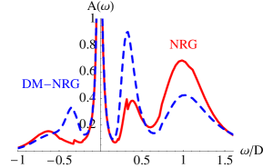
Figure 5: Comparison of spectral densities computed by the conventional NRG and by the DM-NRG for parameters where the conventional NRG approach has difficulties: $t_{d}/D=0.3$, $U/D=1$, $\Gamma/D=0.03$, $\delta/D=0.48$. Note the discontinuities in the spectral density calculated using the conventional NRG. At low frequencies both method produce identical results, so we do not show the Kondo peak which exceeds the vertical scale of the plot. In this calculations, the effective temperature is zero.

We observed that the spectral density calculation using the conventional NRG approach Costi et al. (1994) fails for our model. The spectral densities manifest spurious discontinuities and the normalization sum rule is violated for some choices of model parameters (Fig. 5). This happens because at the early stages of the NRG iteration the lowest energy state does not yet correspond to the true ground state. We found that we obtain correct results using the density-matrix NRG technique Hofstetter (2000), which remedies the shortcomings of the conventional approach. We succeeded in implementing this technique with eigenstates defined within subspaces with well defined occupation $Q$ and total spin $S$, as opposed to well defined occupation and total spin component $S_{z}$ (see the Appendix). The improvement in numerical efficiency is sufficient to enable consideration of more complex systems, such as the double quantum dot.

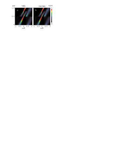
Figure 6: Zero-temperature spectral density $\rho_{d}(\omega)$ sweeps for $t_{d}/D=0.3$. a) Spectral density calculated using the conventional NRG approach. b) Spectral density calculated using the density-matrix NRG approach. Note that the vertical line, representing the Kondo peak, has been artificially broadened. Its true width is given by $T_{K}$.

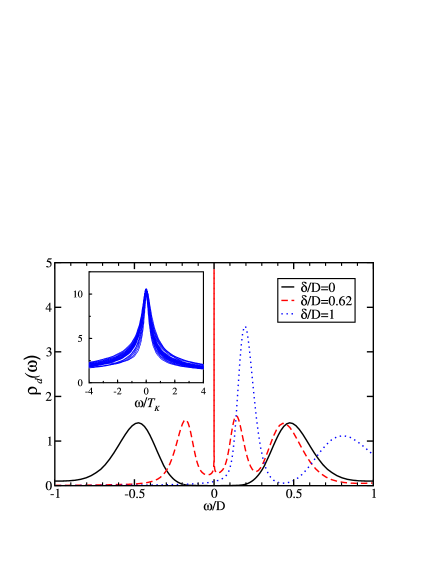
Figure 7: Three zero-temperature spectral densities $\rho_{d}(\omega)$ for $t_{d}/D=0.3$: at the particle-hole symmetric point $\delta/D=0$, in the Kondo regime $\delta/D=0.62$ and in the empty-orbital regime $\delta/D=1$. Inset: Scaling of spectral densities $\rho_{d}(\omega/T_{K})$ in the Kondo region $0.52<\delta<0.76$. Parameters are as in Fig. 2.

In Fig. 6 we present sweeps of $\rho_{d}(\omega)$ calculated using both approaches. In vast regions of the plot the results are in perfect agreement. The differences appear for those values of $\delta$ where the ground state changes. Three characteristic spectral density curves calculated using the DM-NRG are shown in Fig. 7.

Features in the spectral density sweeps can be easily interpreted using eigenvalue diagram in Fig. 3. At low temperatures and for constant $\delta$, spectral density $A(\omega)$ will be high whenever the energy difference $\Delta E=E_{1}-E_{0}$ between the ground state $(0)$ and an excited state $(1)$ is equal to $+\omega$ (particle excitations, $Q_{1}=Q_{0}+1$, $S_{1}=S_{0}\pm\tfrac{1}{2}$) or to $-\omega$ (hole excitations, $Q_{1}=Q_{0}-1$, $S_{1}=S_{0}\pm\tfrac{1}{2}$). At $\delta=0$ two broad peaks are seen located symmetrically at $\omega\sim\pm\delta_{1}$ (see Fig. 6 and Fig. 7, at $\delta/D=0$). At this point the model is particle-hole symmetric and therefore $E(Q,S,r)=E(-Q,S,r)$ for all $Q,S,r$. Consequently, the spectrum is also symmetric, $\rho_{d}(\omega)=\rho_{d}(-\omega)$. With increasing $\delta$, the particle excitation energy $E(1,\tfrac{1}{2},0)-E(0,0,0)$ increases and the corresponding peak quickly washes out. The hole excitation energy $E(-1,\tfrac{1}{2},0)-E(0,0,0)$ decreases and the peak gains weight.

At $\delta=\delta_{1}$, $E(0,0,0)=E(-1,\tfrac{1}{2},0)$ (point $A$ in Fig. 3) and the system enters the Kondo regime: a sharp many-body resonance appears which remains pinned at the Fermi level throughout the Kondo region (see Fig. 6 and Fig. 7, at $\delta/D=0.62$). Kondo effect occurs whenever the ground state is a doublet, $S=1/2$, and there are excited states with $S^{\prime}=0,1$, $Q^{\prime}=Q\pm 1$. We recognize such regions by characteristic triangular level crossings in the eigenvalue diagram, one of which is marked as triangle $ABC$ in Fig. 3. The high-energy peaks at $\omega=E(0,0,0)-E(-1,\tfrac{1}{2},0)>0$ and $\omega=E(-1,\tfrac{1}{2},0)-E(-2,0,0)<0$ in the spectral density are also characteristic: they correspond to particle and hole excitations that are at the heart of the Kondo effect.

In the case of the DQD we also see additional structure for $\delta_{1}<\delta<\delta_{2}$: a broad peak at $\omega=E(0,1,0)-E(-1,\tfrac{1}{2},0)$ which corresponds to virtual triplet excitations from the ground state. These excitations could also be taken into account in the calculation of the effective exchange interaction, Eq. (9), however due to their high energy, they only lead to an exponentially small renormalization of the Kondo temperature, which may be neglected.

In the inset of Fig. 7 we show scaling of Kondo peaks vs. $\omega/T_{K}$. In the case of perfect scaling, all curves should exactly overlap. However, Kondo temperatures of different peaks differ by almost four orders of magnitudes, as seen in Fig. 4b. Moreover, Kondo peaks become asymmetric near the edges of the Kondo region, i.e. for $\delta\gtrsim\delta_{1}$ and $\delta\lesssim\delta_{2}$. Note also that for each point in Fig. 4b there is a respective spectral density presented in the inset of Fig. 7.

III.3 Effect of the on-site-energy splitting

In real double quantum dot systems, it is difficult to produce dots and electrodes with identical properties. In particular, it is not easy to achieve equal on-site energies $\delta_{d}=\delta_{a}=\delta$ for a wide range of parameters $\delta$. Therefore it is necessary to study the robustness of the physical regimes with respect to the splitting of the on-site energies.

We now generalize slightly our model to allow for unequal on-site energies by introducing a new parameter, $\kappa$, so that on-site energies are $\delta_{d}=\delta+\kappa$ and $\delta_{a}=\delta-\kappa$. The DQD part of the Hamiltonian is now

$$\begin{split}H_{0}&=(\delta+\kappa)(n_{d}-1)+(\delta-\kappa)(n_{a}-1)\\ &-t_{d}\sum_{\sigma}\left(d^{\dagger}_{\sigma}a_{\sigma}+a^{\dagger}_{\sigma}d_{\sigma}\right)\\ &+\frac{U}{2}(n_{d}-1)^{2}+\frac{U}{2}(n_{a}-1)^{2}\end{split}$$ (11)

Only $\kappa>0$ has to be considered, because $H_{0}(\delta,-\kappa)\to H_{0}(-\delta,\kappa)$ when particle-hole transformation $d^{\dagger}_{\mu}\to d_{\mu},a^{\dagger}_{\mu}\to-a_{\mu}$ is performed.

By diagonalization $H_{0}$ exactly, we find that the effect of $\kappa$ is to shift states while the general eigenvalue structure is maintained and is similar to that shown in Fig. 3. We therefore still expect to see two Kondo peaks as $\delta$ is swept for a constant $\kappa$.

In the limit of large $\kappa$ and for $\delta$ such that $\delta_{d}\sim 0$ and $\delta_{a}\to\pm\infty$, the side-coupled dot becomes irrelevant and we recover the familiar single-impurity Anderson model with conduction plateau in the region $-U/2<\delta_{d}<U/2$ with $T_{K}$ given by Eq. (8) with

$$\rho_{0}J=\frac{2\Gamma}{\pi}\left(\frac{1}{|\delta_{d}-U/2|}+\frac{1}{|\delta_{d}+U/2}\right).$$ (12)

This scenario is corroborated by NRG calculations (Fig. 8). The approach to the limit can be determined using the expressions Eqs. (8) and (9), with $\kappa$ dependent $\alpha(\kappa)$, $\beta(\kappa)$ and $E_{1}(\kappa),E_{2}(\kappa)$. The result is shown in Fig. 9a. The $\kappa$ dependence is non-monotonic, which can be traced to non-monotonic behavior of coefficient $\beta(\kappa)$. At $\kappa/D=1$ the asymptotic value $T_{K}/D=1.04\times 10^{-7}$ is nearly reached.

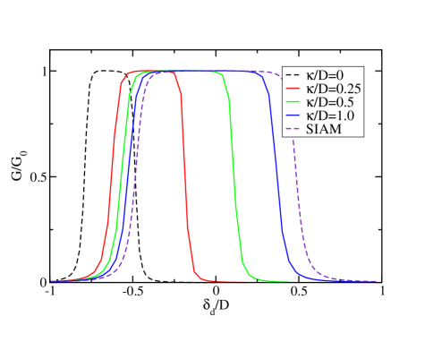
Figure 8: Conductance as a function of gate-voltage $\delta_{d}$ for different gate-voltage asymmetries $\kappa$. Label SIAM corresponds to results for conductance of the corresponding single-impurity Anderson model. The temperature is $T/D=10^{-9}$.

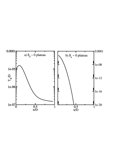
Figure 9: Kondo temperature as a function of $\kappa$ for a) the Kondo plateau at $\delta_{d}\sim 0$ and b) the Kondo plateau at $\delta_{a}\sim 0$. In both cases we calculate the Kondo temperature in the middle of the plateau, where $T_{K}$ is lowest. Parameters are $U/D=1$, $\Gamma/D=0.03$ and $t_{d}/D=0.3$.

In the limit of large $\kappa$, but for $\delta$ such that $\delta_{a}\sim 0$ and $\delta_{d}\to\pm\infty$, the embedded dot will be either fully occupied or empty with very little charge fluctuations, while the side-coupled dot will maintain $S=1/2$ spin moment. This moment will be screened, but due to the suppression of the virtual electron hopping through the dot $d$ the corresponding Kondo temperature rapidly drops with increasing $\kappa$ (Fig. 9b). Keeping the temperature constant and increasing $\kappa$, the Kondo plateau in the region $-U/2<\delta_{a}<U/2$ will therefore quickly evolve into two peaks separated by a Coulomb blockade valley and for very large $\kappa$ it will not conduct at all. This prediction can also be verified using NRG (Fig. 10).

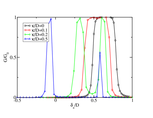
Figure 10: Conductance as a function of gate-voltage $\delta_{a}$ for different gate-voltage asymmetries $\kappa$. The temperature is fixed to $T/D=10^{-9}$ for all $\kappa$.

IV Weak inter-dot coupling

IV.1 Conductance and correlation functions

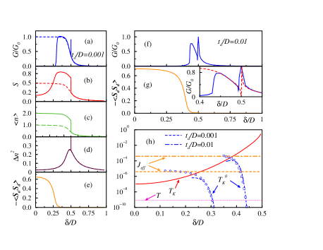
Figure 11: Conductance and correlation functions at $t_{d}/D=0.001$ (a,…,e), $t_{d}/D=0.01$ (f,and g) and a blow-up of f) in the inset of g). Dashed lines in a) represent $G/G_{0}$ and b) $S$ of a single quantum dot with otherwise identical parameters. Dashed line in c) represents $\langle n_{d}\rangle$ of DQD, and finally dashed line in the inset of g) represents the semi-analytical model described in the text. In h) a schematic plot of different temperatures and interactions is presented as explained in the text. NRG values of the gap in $\rho_{d}(\omega)$ at $\omega=0$ and $T\ll T_{K}^{0}$ are presented with open circles and squares for $t_{d}/D=0.001$ and $0.01$ respectively. Values of $J_{\mathrm{eff}}$ and analytical results of $T_{K}^{0}$ are presented with dashed and dot-dashed lines for $t_{d}/D=0.001$ and $0.01$ respectively. For analytical estimates of $T_{K}^{0}$ different values of $\alpha=2.2$ and $1.3$, respectively, were used. Other parameters of the model are $\Gamma/D=0.03,U/D=1$.

We now turn to the limit when $t_{d}\to 0$. Unless otherwise specified, we choose the effective temperature $T$ to be finite, i.e. $T\sim 10^{-9}D$, since calculations at much lower temperatures would be experimentally irrelevant. In this case one naively expects to obtain essentially identical conductance as in the single-dot case. As $\delta$ decreases below $\delta\sim U/2$, $G/G_{0}$ indeed follows result obtained for the single-dot case as shown in Fig. 11a. In the case of DQD, however, a sharp Fano resonance appears at $\delta=U/2$. This resonance coincides with the sudden jump in $S$, $\langle n\rangle$, as well as with the spike in $\Delta n^{2}$, as shown in Figs 11b,c, and d, respectively. Fano resonance is a consequence of a sudden charging of the nearly decoupled dot $a$, as its level $\epsilon$ crosses the chemical potential of the leads, i.e at $\epsilon=0$. Meanwhile, the electron density on the dot $d$ remains a smooth function of $\delta$, as seen from $\langle n_{d}\rangle$ in Fig 11c. With increasing $t_{d}$, the width of the resonance increases, as shown for $t_{d}/D=0.01$ in Fig. 11f. For $t_{d}\gtrsim 0.1$, the resonance merges with the Kondo plateau and disappears (see Fig. 2a).

The resonance at $\delta\sim U/2$ can be explained using a simple semi-analytical model. For $t_{d}=0$, we write the exact Green’s function of the impurity $d$ at $\omega=0$ as ${\cal G}^{0}_{d}=1/(i\Gamma-\Gamma\cot\phi)$ Langreth (1966), where $\phi$ is the scattering phase shift for single impurity model that we calculate using NRG. The side-coupled dot is taken into account using perturbation theory. We obtain full Green’s function from the Dyson’s equation

$${\cal G}_{d}={\cal G}_{d}^{0}/(1-t_{d}^{2}{\cal G}_{a}^{0}{\cal G}_{d}^{0}).$$ (13)

For the Fano resonance at $\epsilon=\delta-U/2\sim 0$, we keep only the low-energy pole in the Green’s function,

$${\cal G}_{a}^{0}(\omega)\approx\tfrac{z}{\omega-\epsilon+i\eta},$$ (14)

where $z=\tfrac{1}{2}$ for $\epsilon<0$ and $z=1$ for $\epsilon>0$. The conductance is

$$G=G_{0}\frac{2\Gamma^{2}\epsilon^{2}\sin^{2}\phi}{z^{2}t_{d}^{4}+2\Gamma^{2}\epsilon^{2}-z^{2}t_{d}^{4}\cos(2\phi)-2zt_{d}^{2}\epsilon\Gamma\sin(2\phi)}.$$ (15)

Results of the NRG calculation are compared to the prediction from Eq. 15 in the inset of Fig. 11g. We see that general features are adequately described, but there are subtle differences due to non-perturbative electron correlation effects. Numerically calculated Fano resonance is wider than the semi-analytical prediction and $G/G_{0}$ does not drop to zero. In particular, from Eq. 15 it follows that $G=0$ at $\delta=U/2$ ($\epsilon=0$) and $G=G_{0}$ at $\delta=U/2+t_{d}^{2}\tan\phi/\Gamma$. This is not corroborated by NRG results, which show maximal conductance at $\delta=U/2$.

We now return to the description of the results presented in Fig. 11a in the regime where $\delta<U/2$. As $\delta$ further decreases, the system enters a regime of the two-stage Kondo effect Cornaglia and Grempel (2005). This region is defined by $J_{\mathrm{eff}}<T_{K}$ (see also Fig. 11h), where $T_{K}$ is the Kondo temperature, approximately given by the single quantum dot Kondo temperature, Eq. 8 with

$$\rho_{0}J=\frac{2\Gamma}{\pi}\left(\frac{1}{|\delta-U/2|}+\frac{1}{|\delta+U/2|}\right).$$ (16)

Just below $\delta<U/2$, $T$ falls in the interval, given by $T_{K}^{0}\ll T\ll T_{K}$, where

$$T_{K}^{0}\sim T_{K}\exp(-\alpha T_{K}/J_{\mathrm{eff}})$$ (17)

denotes the lower Kondo temperature, corresponding to the gap in the spectral density $\rho_{d}(\omega)$ at $\omega=0$ and $\alpha$ is of the order of one Cornaglia and Grempel (2005). Note that NRG values of the gap in $\rho_{d}(\omega)$ (open circles and squares), calculated at $T\ll T_{K}^{0}$, follow analytical results for $T_{K}^{0}(\delta)$ when $J_{\mathrm{eff}}<T_{K}$, see Fig. 11h, while in the opposite regime, i.e. for $J_{\mathrm{eff}}>T_{K}$, they approach $J_{\mathrm{eff}}$.

As shown in Fig. 11a for $0.3D\lesssim\delta<U/2$, $G/G_{0}$ calculated at $T=10^{-9}D$ follows results obtained in the single quantum dot case and approaches value 1. The spin quantum number $S$ in Fig. 11b reaches the value $S\sim 0.8$, consistent with the result obtained for a system of two decoupled spin-1/2 particles, where $\langle{\bf\hat{S}}^{2}\rangle=3/2$. This result is also in agreement with $\langle n\rangle\sim 2$ and the small value of the spin-spin correlation function $\langle{\bf S}_{a}\cdot{\bf S}_{d}\rangle$, presented in Fig. 11c and 11e respectively.

With further decreasing of $\delta$, $G/G_{0}$ suddenly drops to zero at $\delta\lesssim 0.3D$. This sudden drop is approximately given by $T\lesssim T_{K}^{0}(\delta)$, see Figs. 11a and h. At this point the Kondo hole opens in $\rho_{d}(\omega)$ at $\omega=0$, which in turn leads to a drop in the conductivity. The position of this sudden drop in terms of $\delta$ is rather insensitive to the chosen $T$, as apparent from Fig. 11h.

Below $\delta\lesssim 0.25D$, which corresponds to the condition $J_{\mathrm{eff}}\sim T_{K}(\delta)$, also presented in Fig. 11h, the system crosses over from the two stage Kondo regime to a regime where spins on DQD form a singlet. In this case $S$ decreases and $\langle{\bf S}_{a}\cdot{\bf S}_{d}\rangle$ shows strong antiferromagnetic correlations, Figs. 11b and e. The lowest energy scale in the system is $J_{\mathrm{eff}}$, which is supported by the observation that the size of the gap in $\rho_{d}(\omega)$ (open circles in Figs. 11h) is approximately given by $J_{\mathrm{eff}}$. The main difference between $t_{d}/D=0.001$ and $t_{d}/D=0.01$ comes from different values of $J_{\mathrm{eff}}=4t_{d}^{2}/U$. Since in the latter case $J_{\mathrm{eff}}$ is larger, the system enters the AFM singlet regime at much larger values of $\delta$, as can be seen from comparison of Figs. 11g and f. Consequently, the regime of enhanced conductance shrinks.

IV.2 Effect of the on-site-energy splitting

We again explore the effect of unequal on-site energies. Unlike in section III.3, we now introduce the asymmetry so that only the level $a$ is shifted by parameter $\kappa$: $\delta_{d}=\delta$ and $\delta_{a}=\delta+\kappa$. We are mainly interested in the parameter range where for $\kappa=0$ the system exhibits the two-stage Kondo effect.

This study will be conducted by computing the impurity susceptibility

$$\chi_{\mathrm{imp}}(T)=\frac{\left(g\mu_{B}\right)^{2}}{k_{B}T}\left(\langle S_{z}^{2}\rangle-\langle S_{z}^{2}\rangle_{0}\right),$$ (18)

where the first expectation value refers to the system with the double quantum dot, while the second refers to the system without the dots. In traces of $T\chi_{\mathrm{imp}}$, the two-stage Kondo effect manifests as two successive decreases of the susceptibility, at $T\sim T_{K}$ from around $0.5$ to $0.25$ and at $T\sim T_{K}^{0}$ from around $0.25$ to $0$ Cornaglia and Grempel (2005). We now investigate how this behavior changes when $\kappa\neq 0$ by comparing temperature dependent susceptibilities calculated for a range of parameters $\kappa$.

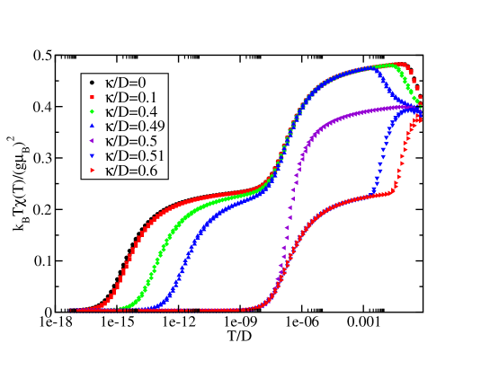
Figure 12: Dynamic magnetic susceptibility $k_{B}T\chi(T)/(g\mu_{B})^{2}$ for different $\kappa$. Parameters are $U/D=1$, $\Gamma/D=0.03$, $t_{d}/D=8\times 10^{-5}$ and $\delta/D=0$. These calculations were performed using a different NRG discretization scheme Campo and Oliveira (2005) with $\Lambda=4$ and keeping 600 states.

We find that the two stage Kondo effect is robust against $\kappa\neq 0$ perturbation. In fact, it survives until $\kappa=U/2$, see Fig. 12. For $\kappa<U/2$ the main effect of $\kappa$ is to reduce the lower Kondo temperature $T_{K}^{0}$. For $\kappa>U/2$, dot $a$ becomes irrelevant at low temperatures and dot $d$ is in the usual Kondo regime.

The transition from $\kappa<U/2$ to $\kappa>U/2$ is continuous despite a rather abrupt change in $\chi_{imp}$ caused by a rapid change in occupation of dot $a$ that occurs with increasing $\kappa$ on an energy scale proportional to $t_{d}^{2}$. For $\kappa=U/2$, $\epsilon_{a}=\delta_{a}-U/2=0$ and the side-coupled dot is in the valence fluctuation regime. For two uncoupled dots, one in local-moment regime and the other in valence-fluctuation regime, the magnetic moment $k_{B}T\chi/(g\mu_{B})^{2}$ is expected to be $1/4+1/6=5/12$. At high temperatures, $\chi$ is indeed in the vicinity of this value.

V Conclusions

In this paper we have explored different regimes of the side-coupled DQD. When quantum dots are strongly coupled, wide regions of enhanced, nearly unitary conductance exist due to the underlying Kondo physics. Analytical estimates for their positions, widths, as well as for the corresponding Kondo temperatures, are given and numerically verified. When two electrons occupy DQD, conductance is zero due to formation of the spin-singlet state which is effectively decoupled from the leads. In this regime most physical properties of the coupled DQD can be predicted using the eigenvalue diagram of the isolated DQD system. This happens because energy separations of different DQD states are much larger than the Kondo temperature. Introducing the on-site-energy splitting between DQD induces new, even though not unexpected effects within the Kondo regime. With increasing level-splitting, the Kondo plateau is expanded when the level of the embedded dot is kept near the local particle-hole limit. In the other case, when, in contrast, the level of the side-coupled dot is kept near the particle-hole limit, Kondo plateau splits at finite $T$ due to abrupt decrease of $T_{K}$ with increasing level-splitting.

When quantum dots are weakly coupled Fano resonance appears in the valence fluctuation regime. Its width is enhanced as a consequence of interactions which should facilitate experimental observation. Unitary conductance exists when two electrons occupy DQD due to a two-stage Kondo effect as long as the temperature of the system is well below $T_{K}$ and above $T_{K}^{0}$. The experimental signature of the two-stage Kondo effect in weakly coupled regime should materialize through the inter-dot-coupling sensitive width of the enhanced conductance vs. gate voltage. Experimental observation of the two-stage Kondo effect would require no external magnetic field as used in Ref. van der Wiel et al. (2002). The inter-dot coupling strength can be experimentally varied using gate electrodes Jeong et al. (2001); Craig et al. (2004); Holleitner et al. (2002); Chen et al. (2004).

*

Appendix A Density-matrix NRG in (Q,S) subspace basis

Density-matrix numerical renormalization group (DM-NRG) Hofstetter (2000) was originally implemented for a NRG iteration that uses subspaces with well defined charge $Q$ and spin projection $S_{z}$ and it was used to determine the effect of magnetic field on spin-projected spectral densities. In the absence of magnetic field, when rotational invariance in the spin space is recovered, it is advantageous to use subspaces with well defined charge $Q$ and spin $S$, which leads to greatly enhanced numerical efficiency.

Here we show how DM-NRG can be implemented in (Q,S) subspace basis in the case of a single conduction channel.

Density-matrix at the last iteration step (estimated using the truncated basis) is:

$$\rho=\frac{1}{Z}\sum_{QSS_{z}\omega}\exp(-\beta E_{QS\omega})|QSS_{z}\omega\rangle\langle QSS_{z}\omega|,$$ (19)

where $\omega$ enumerates different states in each $(Q,S)$ subspace and the grand-canonical statistical sum $Z$ is

$$Z=\mathrm{Tr}\left[\exp(-\beta H)\right]=\sum_{QSS_{z}\omega}\exp(-\beta E_{QS\omega}).$$ (20)

Unitary transformation of states from $N$ to $N+1$-th stage is

$$|QSS_{z}\omega\rangle_{N+1}=\sum_{r\alpha}U_{QS}(\omega|r\alpha)|QSS_{z}r\alpha\rangle_{N+1},$$ (21)

where $U_{QS}$ are the corresponding unitary transformation matrices obtained during the diagonalization step of the NRG and the $|QSS_{z}\alpha r\rangle_{N+1}$ states are defined as Krishna-Murthy et al. (1980)

$$\begin{split}|QSS_{z}r1\rangle_{N+1}&=|Q+1,SS_{z}r\rangle_{N}\\ |QSS_{z}r2\rangle_{N+1}&=uf^{\dagger}_{(N+1)\uparrow}|Q,S-\frac{1}{2},S_{z}-\tfrac{1}{2},r\rangle_{N}\\ &+vf^{\dagger}_{(N+1)\downarrow}|Q,S-\tfrac{1}{2},S_{z}+\tfrac{1}{2},r\rangle_{N}\\ |QSS_{z}r3\rangle_{N+1}&=wf^{\dagger}_{(N+1)\uparrow}|Q,S+\tfrac{1}{2},S_{z}-\tfrac{1}{2},r\rangle_{N}\\ &+yf^{\dagger}_{(N+1)\downarrow}|Q,S+\tfrac{1}{2},S_{z}+\tfrac{1}{2},r\rangle_{N}\\ |QSS_{z}r4\rangle_{N+1}&=f^{\dagger}_{(N+1)\uparrow}f^{\dagger}_{(N+1)\downarrow}|Q-1,SS_{z}r\rangle_{N}|\uparrow\downarrow\rangle,\end{split}$$ (22)

where $f^{\dagger}_{(N+1)\sigma}$ is the creation operator for electrons on the $(N+1)$-th site of the “hopping Hamiltonian” and $u,v,w,y$ are the Clebsch-Gordan coefficients

$$\begin{split}u&=\left(\frac{S+S_{z}}{2S}\right)^{1/2}\\ v&=\left(\frac{S-S_{z}}{2S}\right)^{1/2}\\ w&=-\left(\frac{S-S_{z}+1}{2S+2}\right)^{1/2}\\ y&=\left(\frac{S+S_{z}+1}{2S+2}\right)^{1/2}\end{split}$$

The density matrix in the basis of $|QSS_{z}\alpha r\rangle_{N+1}$ states is

$$\begin{split}\rho&=\sum_{QSS_{z}\omega}\exp(-\beta E_{QS\omega})\sum_{r\alpha,r^{\prime}\alpha^{\prime}}U_{QS}(\omega|r\alpha)U_{QS}(\omega|r^{\prime}\alpha^{\prime})\\ &|QSS_{z}r\alpha\rangle\langle QSS_{z}r^{\prime}\alpha^{\prime}|.\end{split}$$ (23)

We now perform a partial trace over the states on the additional $(N+1)$-th site to obtain projector operators defined on the chain of length $N$. Diagonal projectors (those with $\alpha=\alpha^{\prime}$) are:

$$\begin{split}\mathrm{Tr}_{N+1}\left(|QSS_{z}r1\rangle\langle QSS_{z}r^{\prime}1|\right)&=|Q+1,SS_{z}r\rangle_{N}\langle Q+1,SS_{z}r^{\prime}|_{N}\\ \mathrm{Tr}_{N+1}\left(|QSS_{z}r4\rangle\langle QSS_{z}r^{\prime}4|\right)&=|Q-1,SS_{z}r\rangle_{N}\langle Q-1,SS_{z}r|_{N}\\ \mathrm{Tr}_{N+1}\left(|QSS_{z}r2\rangle\langle QSS_{z}r^{\prime}2|\right)&=u^{2}|Q,S-\tfrac{1}{2},S_{z}-\tfrac{1}{2},r\rangle_{N}\langle Q,S-\tfrac{1}{2},S_{z}-\tfrac{1}{2},r^{\prime}|_{N}\\ &+v^{2}|Q,S-\tfrac{1}{2},S_{z}+\tfrac{1}{2},r\rangle_{N}\langle Q,S-\tfrac{1}{2},S_{z}+\tfrac{1}{2},r^{\prime}|_{N}\\ \mathrm{Tr}_{N+1}\left(|QSS_{z}r3\rangle\langle QSS_{z}r3|\right)&=w^{2}|Q,S+\tfrac{1}{2},S_{z}-\tfrac{1}{2},r\rangle_{N}\langle Q,S+\tfrac{1}{2},S_{z}-\tfrac{1}{2},r^{\prime}|_{N}\\ &+y^{2}|Q,S+\tfrac{1}{2},S_{z}+\tfrac{1}{2},r\rangle_{N}\langle Q,S+\tfrac{1}{2},S_{z}+\tfrac{1}{2},r^{\prime}|_{N}\end{split}$$ (24)

The out-of-diagonal $\alpha=2,\alpha^{\prime}=3$ terms give zero when summed over

$$\begin{split}&\sum_{S_{z}=-S}^{S}\mathrm{Tr}_{N+1}|QSS_{z}r2\rangle\langle QSS_{z}r^{\prime}3|=\\ &=\sum_{S_{z}=-S+1}^{S}\left(-\sqrt{\frac{(S+S_{z})(S-S_{z}+1)}{2S(2S+2)}}+\sqrt{\frac{(S-S_{z}+1)(S+S_{z})}{2S(2S+2)}}\right)\\ &\quad|Q,S-\tfrac{1}{2},S_{z}-\tfrac{1}{2},r\rangle_{N}\langle Q,S+\tfrac{1}{2},S_{z}-\tfrac{1}{2},r^{\prime}|_{N}=0\end{split}$$ (25)

where we took into account that $v_{SS}=0$ and $u_{S,-S}=0$ in order to expand the range of summation index $S_{z}$. Similarly we show that $\alpha=3,\alpha^{\prime}=2$ terms drop.

The $\alpha=\alpha^{\prime}=2$ terms can be simplified after summing over $S_{z}$:

$$\begin{split}&\sum_{S_{z}=-S}^{S}\mathrm{Tr}_{N+1}\left(|QSS_{z}r2\rangle\langle QSS_{z}r^{\prime}2|\right)\\ &=\sum_{S_{z}=-S+1}^{S}\left(u_{SS_{z}}^{2}+v_{S,S_{z}-1}^{2}\right)|Q,S-\tfrac{1}{2},S_{z}-\tfrac{1}{2},r\rangle_{N}\langle Q,S-\tfrac{1}{2},S_{z}-\tfrac{1}{2},r^{\prime}|_{N}\\ &=\frac{2S+1}{2S}\sum_{S_{z}=-(S-\tfrac{1}{2})}^{+(S-\tfrac{1}{2})}|Q,S-\tfrac{1}{2},S_{z}\rangle_{N}\langle Q,S-\tfrac{1}{2},S_{z},r^{\prime}|_{N}\\ \end{split}$$ (26)

The spin multiplicity of $(QS)_{N+1}$ space is $2S+1$, while the spin multiplicity of $(Q,S-\tfrac{1}{2})_{N}$ is $2S$. The factor $(2S+1)/(2S)$ is therefore merely a normalization factor. In the last line we emphasized that in the $N$-site space the $S_{z}$ runs over all permissible values for spin $S-\tfrac{1}{2}$.

By analogy we show that the $\alpha=\alpha^{\prime}=3$ terms also simplify:

$$\begin{split}&\sum_{S_{z}=-S}^{S}\mathrm{Tr}_{N+1}\left(|QSS_{z}r3\rangle\langle QSS_{z}r3|\right)\\ &=\frac{2S+1}{2S+2}\sum_{S_{z}=-(S+\tfrac{1}{2})}^{S+\tfrac{1}{2}}|Q,S+\tfrac{1}{2},S_{z},r\rangle_{N}\langle Q,S+\tfrac{1}{2},S_{z},r^{\prime}|_{N}\end{split}$$ (27)

Again, the spin multiplicity of the $(Q,S+\tfrac{1}{2})_{N}$ space is $2S+2$ and the factor $(2S+1)/(2S+2)$ takes care of the correct normalization.

Non-zero partial traces of projector operators are therefore:

$$\begin{split}&\sum_{S_{z}}\mathrm{Tr}_{N+1}|QSS_{z}r\alpha\rangle\langle QSS_{z}r^{\prime}\alpha^{\prime}|\\ &=\delta_{\alpha\alpha^{\prime}}c_{\alpha}(S)\sum_{S_{z\alpha}}|Q_{\alpha}S_{\alpha}S_{z\alpha}r\rangle_{N}\langle Q_{\alpha}S_{\alpha}S_{z\alpha}r^{\prime}|_{N}\end{split}$$ (28)

with $c_{1}=c_{4}=1$, $c_{2}=\frac{2S+1}{2S}$, $c_{3}=\frac{2S+1}{2S+2}$, $Q_{1}=Q+1$, $Q_{2}=Q_{3}=Q$, $Q_{4}=Q-1$, $S_{1}=S_{4}=S$, $S_{2}=S-\tfrac{1}{2}$, $S_{3}=S+\tfrac{1}{2}$ and corresponding $S_{z\alpha}$ ranges over all possible values for a given $S_{\alpha}$. The reduced density matrix remains diagonal in its $(QS)$ subspace index.

In general we therefore have

$$\begin{split}&\rho^{N+1}_{\mathrm{reduced}}=\sum_{QSS_{z}}\sum_{\omega\omega^{\prime}}C^{QS,N+1}_{\omega\omega^{\prime}}|QSS_{z}\omega\rangle\langle QSS_{z}\omega^{\prime}|\\ &=\sum_{QS}\sum_{\omega\omega^{\prime}}C^{QS,N+1}_{\omega\omega^{\prime}}\sum_{r\alpha,r^{\prime}}U_{QS}(\omega|r\alpha)\\ &U_{QS}(\omega^{\prime}|r^{\prime}\alpha)c_{\alpha}(S)\sum_{S_{z\alpha}}|Q_{\alpha}S_{\alpha}S_{z\alpha}r\rangle_{N}\langle Q_{\alpha}S_{\alpha}S_{z\alpha}r^{\prime}|_{N}.\\ \end{split}$$ (29)

This is to be comapred with

$$\rho^{N}_{\mathrm{reduced}}=\sum_{QSS_{z}}\sum_{rr^{\prime}}C^{QS,N}_{rr^{\prime}}|QSS_{z}r\rangle\langle QSS_{z}r^{\prime}|.$$ (30)

We finally obtain the recursion relation for calculation of coefficients $C^{QS,N}_{rr^{\prime}}$ in the reduced density matrix:

$$C^{QS,N}_{rr^{\prime}} = \sum_{\omega\omega^{\prime}}C^{Q-1,S,N+1}_{\omega\omega^{\prime}}U_{Q-1,S}(\omega|r1)U_{Q-1,S}(\omega^{\prime}|r^{\prime}1)$$ (31)

$$+ \sum_{\omega\omega^{\prime}}C^{Q+1,S,N+1}_{\omega\omega^{\prime}}U_{Q+1,S}(\omega|r4)U_{Q+1,S}(\omega^{\prime}|r^{\prime}4)$$

$$+ \frac{2S+2}{2S+1}\sum_{\omega\omega^{\prime}}C^{Q,S+\tfrac{1}{2},N+1}_{\omega\omega^{\prime}}$$

$$\quad U_{Q,S+\tfrac{1}{2}}(\omega|r2)U_{Q,S+\tfrac{1}{2}}(\omega^{\prime}|r^{\prime}2)$$

$$+ \frac{2S}{2S+1}\sum_{\omega\omega^{\prime}}C^{Q,S-\tfrac{1}{2},N+1}_{\omega\omega^{\prime}}$$

$$\quad U_{Q,S-\tfrac{1}{2}}(\omega|r3)U_{Q,S-\tfrac{1}{2}}(\omega^{\prime}|r^{\prime}3)$$

This is the main result of the derivation. Using known $U_{Q,S}$ matrices, recursion in Eq. (31) is applied after the first NRG run to calculate reduced density matrices for all chain lengths. In another NRG run, the spectral density functions are then calculated with respect to the reduced density matrices:

$$\begin{split}A^{N}_{d\sigma}(\omega)&=\sum_{ijm}\Bigl{(}\langle j|d^{\dagger}_{\sigma}|m\rangle\langle j|d^{\dagger}_{\sigma}|i\rangle\rho^{\mathrm{reduced}}_{im}\\ &+\langle i|d^{\dagger}_{\sigma}|m\rangle\langle j|d^{\dagger}_{\sigma}|m\rangle\rho^{\mathrm{reduced}}_{ji}\Bigr{)}\delta\left(\omega-(E_{j}-E_{m})\right)\end{split}$$ (32)

References

- Jeong et al. (2001) H. Jeong, A. M. Chang, and M. R. Melloch, Science 293, 2221 (2001).
- Craig et al. (2004) N. J. Craig, J. M. Taylor, E. A. Lester, C. M. Marcus, M. P. Hanson, and A. C. Gossard, Science 304, 565 (2004).
- Holleitner et al. (2002) A. W. Holleitner, R. H. Blick, A. K. H uttel, K. Eberl, and J. P. Kotthaus, Science 297, 70 (2002).
- Chen et al. (2004) J. C. Chen, A. M. Chang, and M. R. Melloch, Phys. Rev. Lett. 92, 176801 (2004).
- Hofstetter and Schoeller (2003) W. Hofstetter and H. Schoeller, Phys. Rev. Lett. 88, 016803 (2003).
- Hofstetter and Zarand (2004) W. Hofstetter and G. Zarand, Phys. Rev. B 69, 235301 (2004).
- van der Wiel et al. (2002) W. G. van der Wiel, S. D. Franceschi, J. M. Elzerman, S. Tarucha, L. P. Kouwenhoven, J. Motohisa, F. Nakajima, and T. Fukui, Phys. Rev. Lett. 88, 126803 (2002).
- Granger et al. (2005) G. Granger, M. A. Kastner, I. Radu, M. P. Hanson, and A. C. Gossard, Phys. Rev. B 72, 165309 (2005).
- Kobayashi et al. (2002) K. Kobayashi, H. Aikawa, S. Katsumoto, and Y. Iye, Phys. Rev. Lett. 88, 256806 (2002).
- Kobayashi et al. (2004) K. Kobayashi, H. Aikawa, A. Sano, S. Katsumoto, and Y. Iye, Phys. Rev. B 70, 035319 (2004).
- Bulka and Stefanski (2001) B. R. Bulka and P. Stefanski, Phys. Rev. Lett. 86, 5128 (2001).
- Stefanski et al. (2004) P. Stefanski, A. Tagliacozzo, and B. R. Bulka, Phys. Rev. Lett. 93, 186805 (2004).
- (13) G. A. Lara, P. A. Orellana, J. M. Yanez, and E. V. Anda, cond-mat/0411661.
- Kim and Hershfield (2001) T.-S. Kim and S. Hershfield, Phys. Rev. B 63, 245326 (2001).
- Apel et al. (2004) V. M. Apel, M. A. Davidovich, E. V. Anda, G. Chiappe, and C. A. Busser, Eur. Phys. J. B 40, 365 (2004).
- Kang et al. (2001) K. Kang, S. Y. Cho, J.-J. Kim, and S.-C. Shin, Phys. Rev. B 63, 113304 (2001).
- Cornaglia and Grempel (2005) P. S. Cornaglia and D. R. Grempel, Phys. Rev. B 71, 075305 (2005).
- Vojta et al. (2002) M. Vojta, R. Bulla, and W. Hofstetter, Phys. Rev. B 65, 140405 (2002).
- Glazman and Raikh (1988) L. I. Glazman and M. E. Raikh, JETP Lett. 47, 452 (1988).
- Meir and Wingreen (1992) Y. Meir and N. S. Wingreen, Phys. Rev. Lett. 68, 2512 (1992).
- Wilson (1975) K. G. Wilson, Rev. Mod. Phys. 47, 773 (1975).
- Costi (2001) T. A. Costi, Phys. Rev. B 64, 241310 (2001).
- Krishna-Murthy et al. (1980) H. R. Krishna-Murthy, J. W. Wilkins, and K. G. Wilson, Phys. Rev. B 21, 1003 (1980).
- Hofstetter (2000) W. Hofstetter, Phys. Rev. Lett. 85, 1508 (2000).
- Hewson (1993) A. C. Hewson, The Kondo problem to heavy fermions (Cambridge University Press, 1993).
- Haldane (1978) F. Haldane, J. Phys. C: Solid State Phys. 11, 5015 (1978).
- Costi et al. (1994) T. A. Costi, A. C. Hewson, and V. Zlatic, J. Phys.: Condens. Matter 6, 2519 (1994).
- Langreth (1966) D. C. Langreth, Phys. Rev. 150, 516 (1966).
- Campo and Oliveira (2005) V. L. Campo and L. N. Oliveira, Phys. Rev. B 72, 104432 (2005).