Simulation of a stationary dark soliton in a trapped zero-temperature Bose-Einstein condensate

Abstract

We discuss a computational mechanism for the generation of a stationary dark soliton, or black soliton, in a trapped Bose-Einstein condensate using the Gross-Pitaevskii (GP) equation for both attractive and repulsive interaction. It is demonstrated that the black soliton with a “notch” in the probability density with a zero at the minimum is a stationary eigenstate of the GP equation and can be efficiently generated numerically as a nonlinear continuation of the first vibrational excitation of the GP equation in both attractive and repulsive cases in one and three dimensions for pure harmonic as well as harmonic plus optical-lattice traps. We also demonstrate the stability of this scheme under different perturbing forces.

I Introduction

Solitons are solutions of wave equation where localization is obtained due to a nonlinear interaction and have been observed in optics 1 , water waves 1 , and in Bose-Einstein condensates (BEC) 2 ; vr ; 3 . The bright solitons of BEC represent local maxima 4 and the dark and grey solitons local minima bur ; 5a ; 5b ; 5c . A stationary dark soliton where the local minimum goes to zero value is called a black soliton. There have been experimental study of bright 3 , dark and grey 2 ; vr solitons of BEC. Dark solitons of nonlinear optics 1 are governed by the nonlinear Schrödinger (NLS) equation which is similar to the mean-field Gross-Pitaevskii (GP) equation 7 describing a trapped BEC. More recently, dark solitons have been observed in trapped BECs 2 ; vr .

The one-dimensional NLS equation in the repulsive or self-defocusing case is usually written as 1

$$iu_{t}+u_{xx}-|u|^{2}u=0,$$ (1)

where the time ($t$) and space ($x$) dependences of the wave function $u(x,t)$ are suppressed. This equation sustains the following dark and grey solitons 5 :

$$u(x,t)=r(x-ct)\exp[-i\{\phi(x-ct)-\mu t\}],$$ (2)

with

$$r^{2}(x-ct) = \eta-2\xi^{2}\mbox{sech}^{2}[\xi(x-ct)],$$ (3)

$$\phi(x-ct) = \tan^{-1}[-2\xi/c\hskip 1.42271pt\tanh\{\xi(x-ct)\}],$$ (4)

$$\xi = \sqrt{(2\eta-c^{2})}/2,$$ (5)

where $c$ is the velocity, $\mu$ is a parameter, and $\eta$ is related to intensity. Soliton (2) having a “notch” over a background density is grey in general. It is dark if density $|u|^{2}=0$ at the minimum. At zero velocity the soliton becomes a dark soliton: $|u(x,t)|=\sqrt{\eta}\tanh[\sqrt{(\eta/2)}x]$.

The similarity of the NLS equation (1) to the GP equation of a trapped BEC (Eq. (6) below) imply the possibility of a stationary dark soliton, or a black soliton, in a trapped zero-temperature BEC bur . It has been suggested that the black soliton of a trapped BEC could be a stationary eigenstate of the GP equation bur ; 5b as in the case of the trap-less NLS equation. Here we re-investigate the origin of the black soliton in a trapped zero-temperature BEC and point out that this soliton 5a ; 5b ; 8 ; 9 ; 10 is the first vibrational excitation of the GP equation for both attractive and repulsive atomic interactions and is a stationary eigenstate. We suggest a scheme for numerical simulation of a stationary dark soliton by time evolution of the linear GP equation starting with the analytic vibrational excitation, while the nonlinearity is slowly introduced. We simulate a stationary dark soliton in a harmonic and harmonic plus optical-lattice traps in one and three dimensions. In all cases the simulation proceeds through successive eigenstates of the GP equation. Consequently, the stationary dark soliton in a trapped BEC could be kept stable during numerical simulation. To illustrate the stability of our scheme we also study the breathing oscillation of the stationary dark soliton upon application of different perturbations.

The stationary dark soliton being an excited state is thermodynamically unstable. It is also unstable due to quantum fluctuations z . However, these instabilities are not manifested in the mean-field model. It seems that it will be difficult to generate black solitons experimentally because they are fragile to perturbations, transverse dimensions, quantum effects, and thermal perturbations, etc. Nevertheless, we demonstrate that they are stationary eigenstates of the GP equation and exploit this information to illustrate a simple numerical scheme for their generation. The present numerical scheme has recently been used successfully to simulate the stationary dark solitons of a degenerate boson-fermion mixture bf .

II Black Soliton in a Harmonic Trap

The mean-field dynamics of a trapped BEC is usually described by the time-dependent GP equation 7 . For a strong radial confinement in an axially-symmetric configuration, the GP equation can be reduced to the following quasi-one-dimensional form 8 ; 9 ; 10

$$iu_{t}+u_{xx}-n|u|^{2}u=V(x)u,$$ (6)

where a positive nonlinearity $n$ represents repulsive (self-defocusing) interaction and a negative $n$ represents attractive (self-focusing) interaction. In Eq. (6) $V(x)$ is the external trapping potential. The normalization of the wave function is given by $\int_{-\infty}^{\infty}|u|^{2}dx=1$. The reduction of the GP equation from three to one dimension can be performed in a straightforward fashion for a single- abdul as well as coupled-channel abdul1 cases for small nonlinearity. Nevertheless, for large nonlinearity corrections are needed abdul2 . However, we shall neglect these corrections here.

There is no known analytic solution to Eq. (6) for $V(x)\neq 0$ and $n\neq 0$. Of course, for $n=0$ we have the well-known harmonic oscillator solution for a harmonic trap. However, for $V(x)=0$ and positive $n$, Eq. (6) has the following unnormalizable dark soliton:

$$u(x,t)=\sqrt{2/n}\tanh(x)\exp{(-2it)}.$$ (7)

Soliton (7) has a stationary notch with zero minimum at $x=0$ on a constant background extending to $x=\pm\infty$.

It has been conjectured that a stationary normalizable dark soliton exists in Eq. (6) with a harmonic trap: $V(x)=x^{2}$ and satisfies the same boundary condition as 5c ; 8 ; 9 ; 10

$$u_{\mbox{\small DS}}(x)=N\tanh(x)u_{S}(x),$$ (8)

where $u_{\mbox{\small DS}}(x)$ is the black soliton, $u_{S}(x)$ the ground-state solution to Eq. (6) and $N$ the normalization. The form (8) has been used 9 as an initial guess to a fixed point algorithm that finds the exact numerical stationary solution.

The ansatz (8) has been used as starting guess in numerical studies on dark solitons. Actually, in some applications 9 the Thomas-Fermi (TF) approximation $u_{\mbox{\small TF}}$ 7 has been used in place of $u_{S}$ for positive $n$:

$$u_{S}(x)\approx u_{\mbox{\small TF}}(x)=\sqrt{\mbox{max}(0,[\mu-V(x)]/n)},$$ (9)

where max(,) denotes the larger of the two arguments and $\mu$ is the chemical potential for solution $u_{S}(x)$.

The ansatz (8) is not an eigenstate of Eq. (6). Assuming that it is close to an eigenstate, numerical iteration of Eq. (6) should lead to a stationary dark soliton at large times. Whenever the input (8) is not a good approximation to the stationary dark soliton, oscillations are expected upon iteration. Kevrekidis et al. 9 give a detailed parametric linear stability analysis of the stationary solution obtained through their fixed point iteration scheme varying different parameters, and find windows of stability and windows of instability. They also extend their discussion on instability to the case of an optical-lattice potential. In many cases no stable soliton has been obtained, or an oscillating grey soliton has been found 9 .

One way to achieve a stable soliton with initial guess (8), which is not an eigenstate of Eq. (6), is to include a dissipation in the system. The numerical iteration of a slightly inaccurate solution would generate radiation in general and usually not converge to any stationary state without dissipation. This could be the source of instability in Ref. 9 . In the following, first we study the deficiency of using Eq. (8) in Eq. (6) without dissipation in generating a stationary dark soliton and then illustrate the present alternative scheme, where we use an exact eigenstate of Eq. (6) to generate the stationary dark soliton.

First we performed extensive calculations using ansatz (8) in the time evolution of Eq. (6) using the Crank-Nicholson algorithm 11a for different $n$. We discretize the NLS equation with space step 0.05 and time step 0.0025, which was enough for achieving convergence of a stationary problem. We used accurate numerical solution to $u_{S}(x)$ in place of the TF approximation (9). The present Crank-Nicholson algorithm is appropriate not only for the calculation of stationary states but also for nonequilibrium dynamics 11a with absorptive potential during collapse collapse .

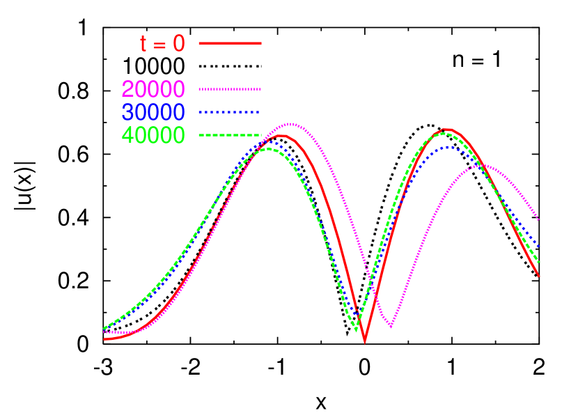
Figure 1: The dark soliton $|u(x)|$ of Eq. (6) with $V(x)=x^{2}$ vs. $x$ for $n=$ 1 obtained by time evolution with input (8) at $t=0$, 10000, 20000, 30000, and 40000. The dark soliton oscillates as a grey soliton without ever converging.

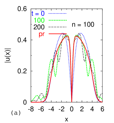
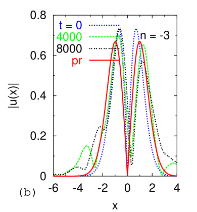
Figure 2: The dark soliton $|u(x)|$ of Eq. (6) with $V(x)=x^{2}$ vs. $x$ for $n=$ (a) 100 and (b) $-3$ obtained by time evolution with input (8) at different times $t$. Also plotted are present stationary results obtained with input (10) marked “pr” (full red line) which do not change with time.

In place of the Crank-Nicholson numerical scheme used in this paper one could also use the method of imaginary time propagation itime for obtaining the stationary states of the GP equation. By replacing the time by an imaginary time variable, the original time-dependent GP equation becomes a diffusion-like equation, and propagation in imaginary time leads to relaxation towards the vibrational ground state. The imaginary time propagator can be expanded in Chebychev polynomials which leads to a stable and efficient scheme. This approach can be easily modified to obtain vibrationally excited states as well. By repeating the relaxation (imaginary time propagation) but filtering out any contribution of the ground state at each time step with anti-periodic boundary conditions, one obtains the first vibrationally excited state. This could be an interesting future work.

Now we perform a direct time evolution of the full GP equation with ansatz (8) as input and show in Fig. 1 the solution at different times for $n=1$. The authors of Ref. 9 are making a different time evolution, e. g., a perturbation of their exact stationary solitary wave with a uniformly distributed random field of amplitude 0.01. As the successive states are not stationary eigenstates these schemes may run into numerical difficulty when the nonlinearity is large. Even for a relatively small nonlinearity of $n=1$, in that approach the solution does not converge at large times: the initial black soliton becomes a grey soliton and oscillates around a mean position at the center of the trap. Although the wave-function density is symmetric at $t=0$, it becomes non-symmetric with the evolution of time. This makes the black soliton to oscillate as a grey soliton upon time evolution before being destroyed eventually for much larger values of time $t$. This trouble as noted in Fig. 1 increases with the increase of nonlinearity $n$.

To circumvent the above-mentioned problem, we find a direct solution to Eq. (6) for the stationary dark soliton with the asymptotic boundary condition implicit in Eq. (8), e. g., $u_{\mbox{\small DS}}(x)\sim x$ as $x\to 0$ and $u_{\mbox{\small DS}}(x)\to 0$ as $x\to\pm\infty$. The solution satisfying these conditions is the nonlinear evolution of the first vibrational excitation of the linear oscillator, obtained by setting $n=0$ in Eq. (6):

$$u_{1}(x,t)=\sqrt{(2/\sqrt{\pi})}x\exp(-x^{2}/2)\exp(-3it).$$ (10)

The possible stationary dark soliton of Eq. (6) can be obtained by time evolution of the GP equation with $u_{1}(x,0)$ as input at $t=0$, setting $n=0$. During time evolution the nonlinearity $n$ should be slowly introduced until the desired nonlinearity is achieved. In this work we increased $n$ by 0.001 at each time propagation, which was sufficient for convergence. By this procedure a stationary dark soliton could be obtained for very large $n$.

Next we compare the time evolution of the dark soliton using conventional ansatz (8) and the present suggestion based on Eq. (10). The results of numerical simulation using the two schemes are plotted in Figs. 2 (a) and (b) for $n=100$ and $-3$ at different times. We show results for these two $n$, as we found that convergence was more difficult for negative $n$ and large positive $n$ values. The case $n=-3$ discussed here is specially interesting as we demonstrate, contrary to popular belief, that dark solitons of a trapped quasi-one-dimensional BEC could be stationary for attractive interactions as well. The iterative solution using Eq. (8) may execute oscillation on time evolution, whereas the solution from input (10) remains stationary on time evolution as the system passes through successive eigenstates and results in a stationary dark soliton of the full NLS equation. In Figs. 2 we show the result for the soliton using the present procedure only at $t=0$ as this result does not change with time. The result based on Eq. (8) oscillates on time evolution as can be found from Figs. 2. However, the oscillation is not so severe for small repulsive $n$ (not shown). The oscillation increases for large repulsive $n$ as well as for attractive nonlinearity. From Figs. 1 and 2 we see that for small $n$ the oscillation is severe for $t>10000$ whereas for large $n(=100)$ it is disturbing even for $t=100$. From Figs. 2 we find that a direct numerical solution for the first excited state of Eq. (6) is the stationary dark soliton that we look for.

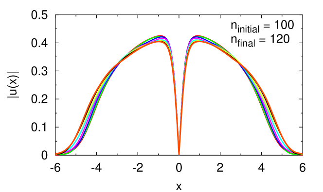
Figure 3: The stationary dark soliton $|u(x)|$ of Fig. 2 (a) at times $t=0,10000,20000,30000,40000,50000$ calculated using the present scheme with input (10) as $n$ is suddenly changed from 100 to 120 at $t=0$.

The fact that a certain numerical scheme converges to a stationary state may not necessarily signify its stability. Although the dark solitons in our study are formed as eigenstates of the nonlinear equation (6), one needs to demonstrate their stability under perturbation. First we suddenly modify the nonlinearity $n$ of Eq. (6) after the dark soliton is obtained and study the resultant dynamics for the dark soliton of Fig. 2 (a). In the case of the dark soliton of Fig. 2 (a) calculated using our scheme based on Eq. (10) we suddenly jump the nonlinearity $n$ from 100 to 120 after the soliton is formed and observe its dynamics for 50000 units of time. The resultant dynamics is shown in Fig. 3.

From Fig. 3 we find that even after giving a perturbation by changing $n$, the resultant stationary dark soliton remains stable for a large interval of time (50000 units of time) performing small breathing oscillation during which the central notch or minimum of the stationary dark soliton remains absolutely stable at $x=0$. From Figs. 2 we find that in the iterative time evolution method based on ansatz (8) the dark soliton may develop dynamical instability with the central notch executing quasi-periodic oscillation around $x=0$ on time evolution before being destroyed without any perturbation whatsoever in a much smaller interval of time than that considered in Fig. 3.

In addition to the perturbation studied in Fig. 3 we make two different types of perturbation to strengthen our claim of stability. First we study the dynamics by increasing the strength of the harmonic trap by $20\%$: (i) $x^{2}\to 1.2x^{2}$. These perturbations are symmetric around $x=0$ which may not displace the notch in the dark soliton from $x=0$. We consider also the asymmetric perturbation (ii) $u(x)\to u(x)+0.02\times\mbox{abs}(u(x))$ where abs denotes absolute value. As $u(x)$ for the dark soliton is antisymmetric around $x=0$, perturbation (ii) destroys the symmetry around $x=0$. From Figs. 2 and 3 it is realized that it would be more difficult to have stability for a large nonlinearity. Hence in the next two studies on stability we consider only $n=100$. The remarkable stability of the soliton under perturbations (i) and (ii) above is illustrated in Figs. 4 (a) and (b). Of these even the asymmetric perturbation (ii) leaves the central notch of the stationary dark soliton essentially stable at $x=0$. The dynamics at small times in Fig. 4 (b) shows some asymmetry, which, instead of increasing, disappears at large times. From Fig. 2 (a) we find that the dark soliton calculated using ansatz (8) is destroyed after a small time of $t=100$ without any perturbation whatsoever.

There seems to be one difference between the behavior of the dark soliton in Figs. 4 and the corresponding behavior of a BEC in a trap. With a sudden change of the trap frequency, a BEC executes breathing oscillation where the central density fluctuates 11a . In Fig. 4 (a) we also observe a similar breathing oscillation. However, in this case because of the nature of the black soliton the central density remains zero, at least for a small change of trap frequency. In Fig. 4 (b) the dark soliton is given a asymetric displacement initially. Because of the stationary nature of the initial dark soliton, the initial oscillation tends to disappear after some time as the dark soliton settles to a stationary configuration. The scenario in Figs. 4 should change upon a large perturbation.

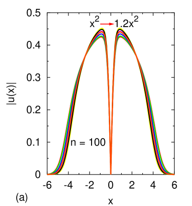
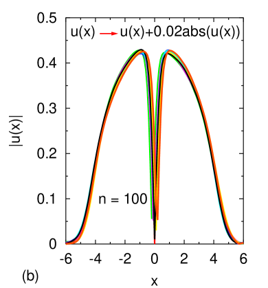
Figure 4: The dark soliton $|u(x)|$ of Fig. 2 (a) at times $t=10000,20000,30000,40000,50000$ calculated using the present scheme with input (10) (a) as the harmonic oscillator potential $x^{2}$ is increased by $20\%:x^{2}\to 1.2x^{2}$ and (b) under the change $u(x)\to u(x)+0.02\times\mbox{abs}(u(x))$ at $t=0$.

III Harmonic Plus Optical-Lattice Traps

Now we consider the stationary dark soliton in a harmonic plus optical-lattice traps. A periodic optical-lattice trap is usually generated by a standing-wave laser beam of wave length $\lambda$. In experiments the following superposition of a harmonic plus optical-lattice traps has been used 9 ; cata :

$$V(x)=kx^{2}+V_{0}\sin^{2}(2\pi x/\lambda).$$ (11)

Here $V_{0}$ is the strength of the optical-lattice potential. We have introduced a parameter $k$ to control the strength of the harmonic potential.

The search for a stationary dark soliton in potential (11) is performed by introducing this potential in Eq. (6). For this purpose we use the input $u_{1}(x,0)$ of Eq. (10) in Eq. (6) with $n=V_{0}=0$ and perform time evolution using the Crank-Nicholson scheme 11a . Again the discretization was performed with a space step 0.05 and time step 0.0025 except for the calculation reported in Fig. 6 where we had to take a space step 0.02 and time step 0.0004. In the course of time evolution the appropriate nonlinearity and the optical-lattice potential are switched on slowly. Then the time evolution of the resultant equation is carried on until a converged solution is obtained. The results of the calculation for different $n$ are shown in Figs. 5. These results are stationary and do not change with time evolution in the interval $t=0$ to $t=$ 100000.

However, it was more difficult to obtain convergence when nonlinearity $n$ or strength $V_{0}$ increases past 40. For small $n(=1,10)$ convergence could be easily obtained for $V_{0}$ up to 80 or so. For larger $n(=20)$ we could obtain convergence for $V_{0}$ up to 40 or so. When both $n$ and $V_{0}$ are increased, smaller space and time steps are needed for convergence. This is understandable as a large nonlinearity with a strong optical-lattice potential could seriously jeopardize the numerical accuracy. There is no such difficulty if the optical-lattice potential is removed. If $\lambda$ is reduced there is no convergence difficulty, so long as a finer discretization mesh is used.

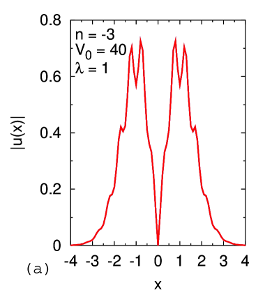
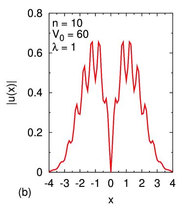
Figure 5: The stationary dark soliton $|u(x)|$ of Eq. (6) with potential (11) with $k=\lambda=1$ vs. $x$ for $n=$ (a) $-3$ and (b) 10 with strength $V_{0}$ of potential (11) given in respective figures. The plotted wave function remains stationary for time evolution of Eq. (6) over 100000 units of time $t$.

The possibility of generating dark solitons in a BEC with a harmonic plus optical-lattice traps (11) has also been investigated by other authors. Kevrekidis et al. 9 obtained stable solitons for their parameters (chemical potential, $\lambda$ etc.) for a very weak trap $V(x)=kx^{2}$ with $k<0.01$. In this study, we could obtain such solutions for our parameter values including $k=1$.

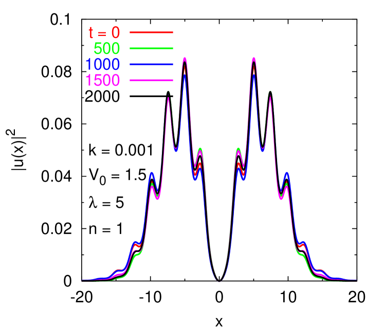
Figure 6: The probability density $|u(x)|^{2}$ of the stationary dark (black) soliton of Eq. (6) with potential (11) with $k=0.001$, $V_{0}=1.5$ and $\lambda=5$ vs. $x$ at different times. The dark soliton with a zero at $x=0$ remains stable for a long time time without executing quasi-periodic oscillation.

In view of the present study, it seems that the instability noted in Ref. 9 could be due to the use of an initial non-stationary state, e. g. (8), to generate the final stationary dark soliton. To substantiate our claim we consider a specific case highlighted by Kevrekidis et al. 9 as an example of instability of the dark soliton in an harmonic plus optical-lattice traps, e.g., for $V(x)=kx^{2}$ with $k=0.001$, $V_{0}=1.5$, and $\lambda=5$ in Eq. (11).

We repeated the above calculation of Kevrekidis et al. 9 using our approach. Because of the small value of $k$, the size of the condensate is much larger in this case compared to the condensates studied above and we had to take a much larger number of mesh points which results in large computing time and slower convergence. However, no quasi-periodic oscillation of the position of the minimum of the dark soliton was observed at large times. The present result is shown in Fig. 6 at different times. The central density in our calculation remains strictly zero over large time scales ($t>2000$), whereas the calculation of Kevrekidis et al. 9 becomes unstable for $t>500$ with the notch of the dark soliton executing quasi-periodic oscillation. There is a difference in the two results, however, which prohibits us to make a quantitative comparison of the two calculations. In the present work the the wave function is normalized to unity, whereas in Ref. 9 the chemical potential has been fixed to unity. However, here we did not use a random perturbation to test the stability of the black soliton.

IV Black Soliton in Three Dimensions

To further fortify the claim of numerical stability of our scheme we next test it in an axially-symmetric three-dimensional BEC under harmonic as well as optical-lattice traps. We consider the following GP equation for the BEC wave function $\psi(x,y;t)\equiv\phi(x,y;t)/x$ at radial position $x$, axial position $y$ and time $t$: cata2

$$\biggr{[} -i\frac{\partial}{\partial t}-{\frac{\partial^{2}}{\partial x^{2}}+\frac{1}{x}\frac{\partial}{\partial x}-\frac{\partial^{2}}{\partial y^{2}}}+\frac{1}{4}(x^{2}+\nu^{2}y^{2})-\frac{1}{x^{2}}$$ (12)

$$+ \frac{4\pi^{2}\kappa}{\lambda^{2}}\cos^{2}\frac{2\pi y}{\lambda}+n\left|\frac{\phi({x,y};t)}{x}\right|^{2}\biggr{]}\phi({x,y};t)=0,$$

with normalization

$$2\pi\int_{-\infty}^{\infty}dy\int_{0}^{\infty}xdx|\psi(x,y;t)|^{2}=1,$$ (13)

where $(x^{2}+\nu^{2}y^{2})/4$ is the axial harmonic trap and $(4\pi^{2}\kappa/\lambda^{2})$ $\cos^{2}(2\pi y/\lambda)$ the optical-lattice potential. Here length and time are expressed in units of $l/\sqrt{2}\equiv\sqrt{\hbar/(2m\omega)}$ and $\omega^{-1}$. respectively, with $\omega$ the radial trap frequency, $m$ the atomic mass, $\nu$ the axial parameter, and $n=8\pi\sqrt{2}N_{0}a/l$ the scaled nonlinearity, where $N_{0}$ is the number of atoms and $a$ the scattering length. The numerical solution is calculated by the Crank-Nicholson discretization scheme where we used as in Ref. 11a a space step of 0.1 in both radial and axial directions and a time step of 0.001. The stationary dark soliton we are looking for is a nonlinear extension of the following solution of Eq. (12) with $n=\kappa=0$:

$$\phi(x,y)=\left(\frac{\nu}{2\pi}\right)^{3/4}xy\exp[-(x^{2}+\nu y^{2})/4],$$ (14)

and can be found in a regular fashion by time evolution of Eq. (12) with $n=\kappa=0$ with Eq. (14) as the initial solution. This solution has a notch at $y=0$ in the axial $y$ direction. In the course of time evolution the nonlinearity $n$ and the optical-lattice strength $\kappa$ are slowly introduced until the final values of these parameters are attained.

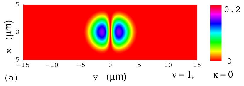
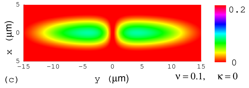
Figure 7: Contour plot of the wave function $|\psi(x,y)|$ of the black soliton of Eq. (12) with harmonic trap alone for (a) $\nu=1$, (b) $\nu=0.4$, and (c) $\nu=0.1$, and $n=100$.

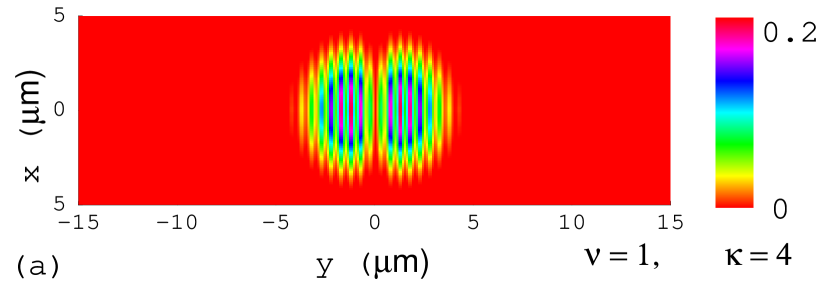
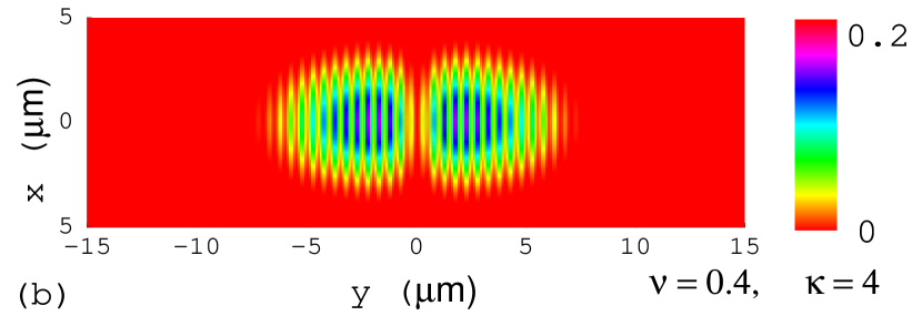
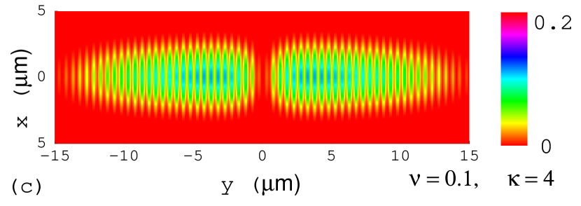
Figure 8: Contour plot of the black-soliton wave function $|\psi(x,y)|$ of Eq. (12) with with $\kappa=4$, $\lambda=1$ and (a) $\nu=1$, (b) $\nu=0.4$, and (c) $\nu=0.1$, and $n=100$.

In this study we take the atoms to be ⁸⁷Rb and a final nonlinearity $n=100$ together with $\omega=2\pi\times 90$ Hz so that $l/\sqrt{2}\approx 0.8$ $\mu$m. First we study the generation of a stationary dark soliton in the harmonic trap alone by setting $\kappa=0$ in Eq. (12) for three values of $\nu=1,0.4$ and 0.1. Contour plots of the wave function $\psi(x,y)$ of the stationary dark soliton in these three cases are exhibited in Figs. 7 (a), (b), and (c), respectively, where the central notch appears prominently and does not oscillate upon time evaluation.

Next we study the stationary dark soliton in the above problem in the presence of an optical-lattice potential with $\kappa=4$ and $\lambda=1$ in addition to the above harmonic potential. The contour plots of the stationary dark soliton in this case are shown in Figs. 8. In addition to the more prominent notch at the center signaling a stationary dark soliton, there are periodic lines along the axial direction due to the optical-lattice potential. This should be contrasted with the similar wave function in one dimension exhibited in Figs. 5 and 6, where there is also periodic modulation of the wave function due to the optical-lattice potential. Needless to say that these dark solitons in three-dimensions are stationary solutions of the GP equation and do not exhibit instability upon time evolution.

V Conclusion

We show that the stationary dark (black) soliton of a trapped zero-temperature BEC is actually a nonlinear extension of the first vibrational excitation of the linear problem obtained by setting $n=0$ in Eq. (6). Based on this, we suggest a time-evolution calculational scheme starting from the linear problem with the harmonic potential alone while the nonlinearity and any additional potential (such as the optical-lattice potential) are slowly introduced during time evolution. This results in a stable numerical scheme for the stationary dark soliton as during time evolution the system always passes through successive stationary eigenstates of the nonlinear GP equation until the desired stationary dark soliton is obtained also as a stationary eigenstate of the final GP equation. The present approach is equally applicable to both repulsive and attractive interactions in one and three dimensions and eliminates the so called dynamical instability of the dark soliton in the presence of a trap and yields a robust stationary dark soliton. To demonstrate the robustness of the present numerical scheme, we illustrate the stable prolonged breathing oscillation of the dark soliton upon the application of a perturbation. We have presented our results in a dimensionless time unit. In a typical experimental situation this unit corresponds to about 1 ms. The stability of the dark soliton during few thousand units of time as considered in this paper is sufficient for this purpose. Time scales beyond a few seconds are completely unrealistic in this context, since the condensate only lives for about 15 seconds, with the soliton predicted to have a much shorter ’lifespan’ due to thermal and quantum fluctuations even at very low temperatures.

We thank Dr. V. V. Konotop and Dr. N. P. Proukakis for helpful e-mails. The work was supported in part by the CNPq and FAPESP of Brazil.

References

- (1) Y. S. Kivshar, G. P. Agrawal, Optical Solitons - From Fibers to Photonic Crystals. Academic Press, San Diego, 2003.
- (2) J. Denschlag, J. E. Simsarian, D. L. Feder, C. W. Clark, L. A. Collins, J. Cubizolles, L. Deng, E. W. Hagley, K. Helmerson, W. P. Reinhardt, S. L. Rolston, B. I. Schneider, W. D. Phillips, Science 287, 97 (2000); S. Burger, K. Bongs, S. Dettmer, W. Ertmer, K. Sengstock, A. Sanpera, G. V. Shlyapnikov, M. Lewenstein, Phys. Rev. Lett. 83, 5198 (1999).
- (3) B. P. Anderson, P. C. Haljan, C. A. Regal, D. L. Feder, L. A. Collins, C. W. Clark, E. A. Cornell, Phys. Rev. Lett. 86, 2926 (2001).
- (4) K. E. Strecker, G. B. Partridge, A. G. Truscott, R. G. Hulet, Nature (London) 417, 150 (2002); L. Khaykovich, F. Schreck, G. Ferrari, T. Bourdel, J. Cubizolles, L. D. Carr, Y. Castin, C. Salomon, Science 296, 1290 (2002).
- (5) V. M. Pérez-García, H. Michinel, H. Herrero, Phys. Rev. A 57, 3837 (1998); S. K. Adhikari, New J. Phys. 5, 137 (2003).
- (6) S. A. Morgan, R. J. Ballagh, K. Burnett, Phys. Rev. A. 55, 4338 (1997).
- (7) A. E. Muryshev, H. B. van Linden van den Heuvell, G. V. Shlyapnikov, Phys. Rev. A 60, R2665 (1999).
- (8) T. Busch, J. R. Anglin, Phys. Rev. Lett. 84, 2298 (2000).
- (9) D. J. Frantzeskakis, G. Theocharis, F. K. Diakonos, P. Schmelcher, Y. S. Kivshar, Phys. Rev. A 66, 053608 (2002); J. Dziarmaga, Z. P. Karkuszewski, K. Sacha, J. Phys. B 36, 1217 (2003); J. Dziarmaga, K. Sacha, Phys. Rev. A 66, 043620 (2002).
- (10) F. Dalfovo, S. Giorgini, L. P. Pitaevskii, S. Stringari, Rev. Mod. Phys. 71, 463 (1999).
- (11) P. G. Drazin, R. S. Johnson, Solitons: An Introduction. Cambridge University Press, Cambridge, 1989.
- (12) R. D’Agosta, B. A. Malomed, C. Presilla, Phys. Lett. A 275, 424 (2000).
- (13) P. G. Kevrekidis, R. Carretero-González, G. Theocharis, D. J. Frantzeskakis, B. A. Malomed, Phys. Rev. A 68, 035602 (2003).
- (14) P. J. Y. Louis, E. A. Ostrovskaya, Y. S. Kivshar, J. Opt. B 6, S309 (2004); V. A. Brazhnyi, V. V. Konotop, Phys. Rev. A 68, 043613 (2003).
- (15) N. G. Parker, N. P. Proukakis, C. F. Barenghi, and C. S. Adams, J. Phys. B 37, S175 (2004); N. P. Proukakis, N. G. Parker, D. J. Frantzeskakis, C. S. Adams, J. Opt. B 6, S380 (2004).
- (16) J. Dziarmaga, Phys. Rev A 70, 063616 (2004).
- (17) S. K. Adhikari, J. Phys. B 38, 3607 (2005).
- (18) F. K. Abdullaev, R. Galimzyanov, J. Phys. B 36, 1099 (2003).
- (19) S. K. Adhikari, Phys. Rev. A 72, 053608 (2005); J. Phys. B 38, 3607 (2005).
- (20) L. Salasnich, A. Parola, L. Reatto, Phys. Rev. A 65, 043614 (2002).
- (21) S. K. Adhikari, P. Muruganandam, J. Phys. B 35, 2831 (2002); P. Muruganandam, S. K. Adhikari, J. Phys. B 36, 2501 (2003).
- (22) S. K. Adhikari, Phys. Rev. A 71, 053603 (2005).
- (23) H. Wallis, A. Röhrl, M. Naraschewski, A. Schenzle, Phys. Rev. A 55, 2109 (1997); T. Karpiuk, M. Brewczyk, K. Rzazewski, J. Phys. B 35, L315 (2002); B. Damski, Z. P. Karkuszewski, K. Sacha, J. Rzazewski, Phys. Rev. A 65, 013604 (2001); D. L. Feder, C. W. Clark, B. I. Schneider, Phys. Rev. A 61, 011601 (2000); B. I. Schneider, D. L. Feder, Phys. Rev. A 59, 2232 (1999).
- (24) F. S. Cataliotti, S. Burger, C. Fort, P. Maddaloni, F. Minardi, A. Trombettoni, A. Smerzi, M. Inguscio, Science 293, 843 (2001); O. Morsch, J. H. Muller, M. Cristiani, D. Ciampini, E. Arimondo, Phys. Rev. Lett. 87, 140402 (2001).
- (25) S. K. Adhikari, Phys. Rev. A 72, 013619 (2005).