Excitonic pairing between nodal fermions

Abstract

We study excitonic pairing in nodal fermion systems characterized by a vanishing quasiparticle density of states at the pointlike Fermi surface and a concomitant lack of screening for long-range interactions. By solving the gap equation for the excitonic order parameter, we obtain a critical value of the interaction strength for a variety of power-law interactions and densities of states. We compute the free energy and analyze possible phase transitions, thus shedding further light on the unusual pairing properties of this peculiar class of strongly correlated systems.

Since its foundation some fifty years ago, Fermi-liquid theory has been providing a convenient framework for the analysis of conventional metals. Nowadays, however, the quest for departures from classic Fermi-liquid behavior has become one of the central themes in modern condensed matter theory.

In a generic one-dimensional (1D) many-fermion system, an arbitrarily weak short-range repulsive interaction is known to completely destroy the Fermi liquid, thereby giving rise to so-called Luttinger behavior. In higher dimensions (2D and 3D), the Fermi liquid is believed to be more robust, although it is not expected to remain absolutely stable. While in the case of short-range repulsive interactions any deviations from the Fermi liquid are likely to be limited to the regime of infinitely strong couplings, the long-ranged interactions are considered to be generally capable of destroying the Fermi liquid even at finite couplings.

In that regard, a particularly promising case appears to be the class of systems which possess isolated (“nodal”) Fermi points where the quasiparticle density of states (DOS) vanishes. As a result, any long-ranged interaction (whether the bare Coulomb one or that mediated by soft collective modes proliferating near an emergent instability) remains largely unscreened.

Examples of the nodal fermion systems are provided by degenerate semimetals, such as graphite or bismuth, where the conduction and valence bands touch each other at isolated points in the Brillouin zone. In a monolayer of graphite, for example, the two-dimensional fermion excitations with the momenta close to the nodal points have a linear dispersion, and, therefore, can be described in terms of a Dirac-like effective theory. semenoff

Amongst other potential candidates to the nodal liquid scenario are $p$ (such as He₃) and $d$ (such as cuprates) superfluids where the quasiparticle gap has isolated nodes. Yet another example is provided by charge density wave (CDW) insulators, such as dichalcogenides, which are thought to have $f$-wave CDW order. antonio

On general grounds, one might expect behavior manifested by systems supporting nodal quasiparticles to be markedly different from that of fermions with an extended Fermi surface from which a bare long-range interaction would undergo strong screening. In particular, it is conceivable that pairing instabilities which, depending on the sign of the interaction, occur either in the particle-particle (Cooper) or particle-hole (Peierls) channels, develop differently from the conventional BCS scenario.

Barring a handful of counter-examples, most of the previous studies of fermion pairing were limited to the simplest BCS case where the momentum dependence of the corresponding order parameter (except, possibly, for its angular dependence) would be routinely neglected. However, while being generally justified in the case of normal metals with their intrinsic screening, the BCS solution may no longer be applicable in the nodal liquids.

In the present paper, we address the general problem of pairing between the nodal fermions with a generic dispersion $\xi_{p}\propto p^{\eta}$. The latter corresponds to the power-law DOS $\nu(\epsilon)\propto\epsilon^{\beta}$ which vanishes at the nodal Fermi point located at ${\bf p}=0$ and is governed by the exponent $\beta={D/\eta-1}$.

Although below we focus on excitonic pairing pertinent to the case of repulsive interactions, much of the following discussion can be readily adapted to the case of the Cooper instability caused by attraction.

In the particle-hole representation, the inverse fermion Green function reads

$$\hat{G}^{-1}(\omega,{\bf p})=\omega-\mu-{\hat{\tau}}_{3}\xi_{p}+{\hat{\tau}}_{1}\Delta_{p}$$ (1)

where ${\hat{\tau}}_{i}$ is the triplet of the Pauli matrices acting in the particle-hole space, $\mu$ is the chemical potential, and $\Delta_{p}$ is the gap function which describes the anticipated spatially uniform (see the conclusions for a discussion of this assumption) pairing in the Peierls channel caused by a long-ranged repulsive potential with the Fourier transform $U^{(0)}({\bf q})=g_{0}/q^{\eta\alpha}$.

When the nodal fermion polarization $\chi(\omega,{\bf q})$ is taken into account, the renormalized effective interaction assumes the form

$$U(\omega,{\bf q})=\frac{g_{0}}{{q}^{\eta\alpha}+g\chi(\omega,{\bf q})}.$$ (2)

At low (compared to a characteristic scale $\Lambda$ which is of order the maximum span of the Brillouin zone) momenta and still lower frequencies ($\omega/q^{\eta}\to 0$ and $q\to 0$) the one-loop polarization behaves as $\chi(0,{\bf q})\propto q^{D-\eta}$. Thus, under the condition $\alpha\leq\beta$, the effective interaction (2) retains its bare form (except for a finite renormalization of the coupling constant $g_{0}\to g_{0}\left[1+g_{0}\chi(0,{\bf q})/q^{\eta\alpha}\right]^{-1}|_{q\to 0}$ and an additional frequency dependence for $\alpha=\beta$). By contrast, for $\alpha>\beta$ the overscreened effective interaction (2) acquires a universal form governed by the fermion polarization, thereby giving rise to the behavior which is qualitatively similar to that occurring at $\alpha=\beta$.

The gap equation is given by the ${\hat{\tau}_{1}}$-component of the Dyson-Schwinger equation for the fermion propagator (1)

$$\hat{G}^{-1}(\omega,{\bf p})=\hat{G}^{-1}_{0}(\omega,{\bf p})+$$

$$i\int\frac{d\Omega}{(2\pi)}\sum_{\bf q}U(\Omega-\omega,{\bf p}-{\bf q})\hat{G}(\Omega,{\bf q})$$ (3)

where ${\hat{G}}_{0}(\omega,{\bf p})$ is the bare propagator with $\Delta_{p}=0$.

In what follows, we focus on the regime $\alpha\leq\beta$ where, conceivably, the polarization operator may still become important at the momenta of order the upper cutoff set by $\Lambda$. We find, however, that a rapid decrease of $\Delta_{p}$ at large momenta (see below) makes the gap function robust against the inclusion of such high-energy polarization effects. By the same token, a polarization-related frequency dependence (retardation) of the effective interaction does not have a significant impact on the solutions of Eq.(1) and, therefore, will be neglected from now on.

Taking into account the above arguments, we perform the frequency integration in Eq.(3) and take its trace with ${\hat{\tau}}_{1}$, thereby arriving at the integral equation for the momentum (albeit not the frequency) dependent gap function

$$\Delta_{\bf p}=\sum_{{\bf q},\mp}U(0,{\bf p}-{\bf q}){(\mp)\Delta_{\bf q}\over 2E_{q}}\theta({\mu\mp E_{\bf q}}),$$ (4)

where $E_{\bf q}={\sqrt{{\xi_{\bf q}}^{2}+\Delta_{\bf q}^{2}}}$ is the quasiparticle energy, and the sum is taken over all the occupied states in both the valence ($\Omega=-E_{\bf q}$) and conduction ($\Omega=E_{\bf q}$) bands.

Notably, for any $\alpha>0$, a nontrivial momentum dependence of the integral kernel in Eq.(4) rules out the possibility of the standard BCS solution $\Delta_{\bf p}=$ const. While resisting an exact analytical solution for general values of $\alpha$ and $\beta$, Eq.(4) can still be amenable to numerical analysis. However, we find it more physically transparent to resort to an approximate analytical approach which generalizes that of Refs. 3 and 4 and allows one to convert an integral equation into a simpler linear differential one. This method elaborates on the earlier analyses appelquist of the phenomenon of chiral symmetry breaking in 3D relativistic fermion systems that can be thought of as a Lorentz-invariant analog of excitonic pairing.

We start off by observing that, at large momenta, Eq.(4) can be simplified by replacing the kernel $U({\bf p-q})$ with either $U({\bf p})$ or $U({\bf q})$, depending on the relative magnitude of the momenta $\bf q$ and $\bf p$. Next, by changing the integration variable from the momentum $\bf p$ to the quasiparticle energy $\epsilon=E_{\bf p}$ and repeatedly differentiating both sides of Eq.(4), we obtain the linear differential equation

$${d^{2}\Delta(\epsilon)\over d\epsilon^{2}}+{\alpha+1\over\epsilon}{d\Delta(\epsilon)\over d\epsilon}+g{\alpha\Delta(\epsilon)\over\epsilon^{2+\alpha-\beta}}=0,$$ (5)

where $g=g_{0}/[2^{D-1}\pi^{D/2}\Gamma(D/2)]$.

In order for Eq.(5) to be consistent with the original integral Eq.(4), it has be complemented with the boundary conditions

$$\left.{d\Delta(\epsilon)\over d\epsilon}\right|_{\epsilon=\max[\Delta,\mu]}=0$$ (6)

and

$$\left.\Delta(\epsilon)+{\epsilon\over\alpha}{d\Delta(\epsilon)\over dE}\right|_{\epsilon=\Lambda}=0.$$ (7)

In what follows, we refer to Eqs.(6) and (7), respectively, as the infrared (IR) and ultraviolet (UV) boundary conditions.

Although the above approximations can be fully justified only at large momenta, a comparison between the numerical analyses of the original gap equation (4) and the relatively simple approximate solutions of the linearized equation (5) (see below) shows that the latter provide a faithful representation of the solutions to Eq.(4) down to the lowest energies $\epsilon\sim\Delta$.

We first consider the case of half filling ($\mu=0$). The linearized Eq.(5) can be interpreted as the radial Schrödinger equation of the zero energy state in the fictitious $(\alpha+2)$-dimensional spherically symmetrical potential $V(R)=g\alpha/R^{2+\alpha-\beta}$. This analogy suggests that for $0\leq\beta-\alpha<1$ the zero energy solution occurs for couplings $g$ in excess of a finite threshold value $g_{c}$.

This prediction is supported by a direct analysis of Eq.(5) which, for $\alpha>\beta/3$, appears to have an approximate solution of the form

$$\Delta\left(\epsilon\right)=\Delta\left(\frac{\Delta}{\epsilon}\right)^{\gamma(\epsilon)}{\sin\left[\Phi(\epsilon)+\delta\right]\over\sin\delta}$$ (8)

where the prefactor is chosen to satisfy the natural normalization condition $\Delta(\epsilon)|_{\epsilon=\Delta}=\Delta$, and the phase of the trigonometric function is given by the expression

$$\Phi(\epsilon)={1\over r}{\sqrt{\alpha g\epsilon^{2r}-\kappa(\epsilon)/4}}\left[1-(\Delta/\epsilon)^{r}\right]$$ (9)

Here $r=(\beta-\alpha)/2$, the phase shift $\delta=\tan^{-1}[{{\sqrt{4\alpha g\Delta^{2r}-\kappa(\Delta)}}/\alpha}]$ for $\Delta>\left[\kappa(\Delta)/4\alpha g\right]^{1/2r}$, otherwise $\delta=0$, is determined by the IR boundary condition, and the slowly varying functions $\gamma(\epsilon)$ and $\kappa(\epsilon)$ attain the following asymptotic values:

$$\gamma(\Delta)=\alpha/2,~{}~{}~{}~{}~{}~{}\gamma(\Lambda)=(\alpha+\beta)/4$$ (10)

and

$$\kappa(\Delta)=\alpha^{2}-(\alpha-\beta)^{2},~{}~{}~{}~{}~{}~{}\kappa(\Lambda)=\alpha^{2}-{1\over 4}(\alpha-\beta)^{2}.$$ (11)

The maximum (zero-momentum) value of the gap function $\Delta=\Delta(0)$ can be determined from the UV boundary condition (7), which now assumes the form

$$\tan[\Phi(\Lambda)]+{4\over 3\alpha-\beta}{\alpha{\tilde{g}}-\kappa(\Lambda)(\Delta/\Lambda)^{r}/4\over{\sqrt{\alpha{\tilde{g}}-\kappa(\Lambda)/4}}}=0,$$ (12)

where ${\tilde{g}}=g\Lambda^{2r}$.

For $0<\alpha<\beta$, Eq.(12) yields

$$\Delta\sim\Lambda({\tilde{g}}-{\tilde{g}}_{c})^{1/r}$$ (13)

for couplings greater than the critical value

$${\tilde{g}}_{c}\approx{1\over 16\alpha}\left[(\alpha+\beta)^{2}+{\pi^{2}(\beta-\alpha)^{2}}\right]$$ (14)

In the marginal case $\alpha=\beta>0$ and for $g>g_{c}=\alpha/4$ the solution (8) takes the form

$$\Delta(\epsilon)=\Delta\left(\frac{\Delta}{\epsilon}\right)^{\alpha/2}{\sin\left[{\sqrt{\alpha g-\alpha^{2}/4}}\ln(\epsilon/\Delta)+\delta\right]\over\sin\delta},$$ (15)

where $\delta=\tan^{-1}{\sqrt{4(g/\alpha)-1}}$.

In the case $\alpha=\beta=1$, Eq.(15) reproduces the solution that was obtained in Refs. 3 and 4. In this case, the gap given by Eq.(12) shows a behavior reminiscent of that at the Kosterlitz-Thouless (KT) transition in $XY$-symmetrical 2D systems

$$\Delta=\Lambda\exp\left(-{2\pi-4\delta\over{\sqrt{4\alpha(g-g_{c})}}}\right).$$ (16)

A similar behavior has been previously found in the context of 3D relativistic chiral symmetry breaking, in which it was conjectured to signal the onset of a conformally invariant critical regime.appelquist The present discussion shows that the KT-like behavior (16) is not specific to Lorentz-invariant systems. Rather, it appears to be characteristic of the scale invariance of the underlying “radial” gap equation (5).

Next, we introduce a finite chemical potential $\mu$, which, depending on the sign, represents a finite density of either particles or holes. The occupation factor $\theta(\mu\mp E_{q})$ in the right-hand side of Eq.(4) sets a lower limit of momentum integration.

A straightforward analysis shows that at $\epsilon\lesssim\mu$ the solution $\Delta(\epsilon)$ of the gap equation levels off and becomes independent of energy. For $\Delta<\mu$ we then impose the normalization condition $\Delta(\epsilon)|_{\epsilon=\mu}=\Delta$, thereby arriving at the approximate formula for the counterpart of Eq.(8)

$$\Delta(\epsilon)=\Delta\left(\frac{\mu}{\epsilon}\right)^{\gamma(\epsilon)}{\sin\left[\Phi(\epsilon)+\delta\right]\over\sin\left[\Phi(\mu)+\delta\right]},$$ (17)

whereas for $\Delta>\mu$ the solution (8) remains essentially intact. In particular, the marginal (scale-invariant) case $\alpha=\beta$ is now described by the gap function

$$\Delta(\epsilon)=\Delta\left(\frac{\mu}{\epsilon}\right)^{\alpha/2}{\sin({\sqrt{\alpha g-\alpha^{2}/4}}\ln{\epsilon/\Delta}+\delta)\over\sin({\sqrt{\alpha g-\alpha^{2}/4}}\ln{\mu/\Delta}+\delta)}.$$ (18)

After having found the approximate solutions to the gap equation, we now proceed to elucidate the nature of the quantum phase transition which results in the opening of the gap. To that end, we use Eqs.(8) and (18) to compute the free energy functional $F(\Delta,\mu)$.

The presence of the long-ranged forces makes it rather challenging to utilize the conventional Luttinger-Ward approach (for its recent application to a very detailed analysis of the non-BCS energy-dependent superconducting pairing, see Ref. 6). Specifically, a straightforward implementation of this method gives rise to a strongly divergent double momentum integral $\sum_{{\bf p},{\bf q}}\Delta_{p}U^{-1}(0,{\bf p}-{\bf q})\Delta_{q}$ whose kernel is given by the (generally, highly nonlocal) inverse operator $U^{-1}(0,{\bf p})$.

Moreover, an unequivocal identification of the solutions to the gap equation as minima (as opposed to maxima) of $F(\Delta,\mu)$ requires one to compute this functional for all $\Delta$, whereas the previous applications of the Luttinger-Ward and similar techniques have been limited to the evaluation of the free energy $F(\Delta_{0},\mu)$ at its absolute minimum $\Delta_{0}$ (“condensation energy”).chubukov2

As an alternate approach, we employ a field-theoretical technique which has been previously used to investigate the conjectured excitonic instability in pyrolytic graphite.kiev This method makes use of the source function (see Ref. 4 and references therein)

$$J(\Delta)=\left.\left(\Delta(\epsilon)+{\epsilon\over\alpha}{d\Delta(\epsilon)\over d\epsilon}\right)\right|_{\epsilon=\Lambda}$$ (19)

and the order parameter

$$\sigma(\Delta)=Tr[{\hat{\tau}_{1}}\int{d\omega\over 2\pi}\sum_{\bf q}{\hat{G}}(\omega,{\bf q})]=\\ \left.{\epsilon^{\alpha}\over g_{0}}\Delta(\epsilon)\right|_{\epsilon=\Lambda}$$

which both determine the sought-after (regularized) effective potential given by the formula

$$F(\Delta,\mu)=\int^{\Delta}_{0}d\Delta^{\prime}{d\sigma(\Delta^{\prime})\over d\Delta^{\prime}}J(\Delta^{\prime})+F(0,\mu).$$ (20)

The integration constant $F(0,\mu)$ is to be found from the equation for the density of excess particles

$$-{\partial F(\Delta,\mu)\over\partial\mu}=n(\mu)=\sum_{{\bf p},\mp}\theta(\mu\mp E_{p}).$$ (21)

In order to illustrate this approach on a well-known example, we first consider the standard BCS pairing between fermions with a short-range interaction potential and a finite density of states ($\alpha=\beta=0$).

For $\mu=0$ and an arbitrarily weak repulsion, the gap equation (4) yields the conventional BCS-type solution $\Delta(\epsilon)=\Delta_{0}=\Lambda e^{-1/g}$.

For $\mu<\Delta$ the free energy reads

$$F_{>}(\Delta,\mu)={g\Delta^{2}\over 4g_{0}}\left({1\over g}-{1\over 2}-\ln{\Lambda\over\Delta}\right),$$ (22)

whereas for $\Delta<\mu$ one obtains

$$F_{<}(\Delta,\mu)={g\Delta^{2}\over 4g_{0}}\left({1\over g}-{1\over 2}-\ln{\Lambda\over\mu+{\sqrt{\mu^{2}-\Delta^{2}}}}\right)$$

$$-{g\over 2g_{0}}\mu{\sqrt{\mu^{2}-\Delta^{2}}},$$ (23)

the last term being proportional to the particle density $n={1\over 2}{\sqrt{\mu^{2}-\Delta^{2}}}$.

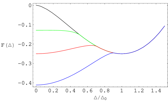
Figure 1: Free energy for $\alpha=\beta=0$ as a function of chemical potential $\mu$ (in units of $\Delta_{0}$): $0$ (black), $0.5$ (green), $1/{\sqrt{2}}$ (red), and $1$ (blue).

The free energy given by Eqs.(23,24) and plotted in Fig.1 exhibits a minimum at $\Delta=\Delta_{0}$ for all $\mu<\mu_{c}=\Delta_{0}/{\sqrt{2}}$ and $g<2$. Upon increasing $\mu$ past the critical value $\mu_{c}$, the minimum jumps discontinuously to the trivial solution $\Delta=0$, consistent with the anticipated first order nature of the transition in question, which is known to be equivalent to the superconducting BCS transition in an external magnetic field.

In the case of Fermi liquids with screened repulsive interactions, the same scenario describes the excitonic instability. It should be noted, however, that the transition driven by a variable density (which provides a more appropriate picture of the system, in which the number of carriers is not fixed) can still be of second order.volkov

This given example demonstrates that by merely evaluating the free energy at the extremal points of $F(\Delta,\mu)$, one may not always be able to distinguish the true absolute minimum from a local one or, worse yet, from a maximum. In that regard, it is worth mentioning the apparent confusion over the nature of the so-called “nontrivial” solution $\Delta={\sqrt{2\Delta_{0}\mu-\Delta^{2}_{0}}}$ that was claimed in Ref. 7 to exist for $\mu>\Delta_{0}/2$. This solution was also invoked in some of the recent studies of the conjectured (weakly ferromagnetic) excitonic insulating state in hexaborides.rice

However, it can be immediately seen from Fig.1 that the extremal point in question is, in fact, a local maximum of the BCS free energy functional. Therefore, it could not have provided a viable solution to the problem of excitonic pairing in a doped semimetal even if the hexaborides belonged to this class of materials (which is now considered rather unlikely from the experimental point of view bennett ).

As the next example, we discuss the case of a short-range potential and a linear density of states ($\alpha=0$, $\beta=1$). Similar to the BCS case, the constancy of the gap function makes the solution to the gap equation [$\Delta(\epsilon)=\Delta_{0}=g^{-1}_{c}-g^{-1}$ for $\mu<\Delta$] trivial.

For $\mu<\Delta$ we obtain

$$F_{>}(\Delta,\mu)={g\over 2g_{0}}{\Delta^{2}}\left({1\over 3}\Delta-{1\over 2}\Delta_{0}\right)$$ (24)

while for $\Delta<\mu$ the free energy incorporating an excess electron density $n(\mu)={1\over 2}(\mu^{2}-\Delta^{2})$ takes the form

$$F_{<}(\Delta,\mu)={g\over 2g_{0}}\left(-{1\over 6}\mu^{3}+{1\over 2}\mu\Delta^{2}-{1\over 2}\Delta_{0}\Delta^{2}\right).$$ (25)

Notably, the terms of order $\Delta^{2}\Lambda$ which are present in both the kinetic and potential contributions cancel each other, and the condensation energy is governed by the fermion states with energies $\epsilon\sim\Delta$.

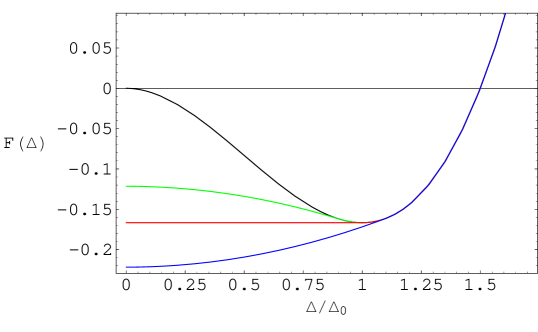
Figure 2: Free energy for $\alpha=0$, $\beta=1$ as a function of chemical potential $\mu$ (in units of $\Delta_{0}$): $0$ (black), $0.9$ (green), $1$ (red), and $1.1$ (blue).

As follows from Eqs.(25,26), the minimum of the free energy plotted in Fig.2 exists for all $g>g_{c}=1/\Lambda$. Interestingly, at $\mu_{c}=\Delta_{0}$ the mean-field free energy becomes independent of $\Delta$ in the entire range $0\leq\Delta\leq\Delta_{0}$, thus signaling the possibility of a continuous transition. It is, however, conceivable that upon accounting for the fluctuations about the mean-field solution one would find the transition in question to be of (possibly, weakly) first order.

Being primarily concerned with the properties of the systems governed by long-ranged interactions, we now move to the case of a linear density of states and the unscreened Coulomb interactions ($\alpha=\beta=1$). Unlike in the previous examples, we now find a nontrivial gap function that conforms to the “scaling-invariant” momentum dependence (15). Computing the free energy for $\Delta<\mu$ we obtain

$$F_{<}(\Delta,\mu)={g\over 2g_{0}}[I_{<}(\Delta,\mu)-I_{<}(\Delta_{0},\mu)$$

$$-{1\over 2}\int^{\mu}_{\Delta}d\omega(\omega^{2}-\Delta^{2})],$$ (26)

where

$$I_{<}(\Delta,\mu)=\mu\int^{\mu}_{0}d\omega\omega{\ln{(\Delta_{0}/\omega)}\left[5-\ln{(\Delta_{0}/\omega)}\right]\over(2+\ln{\mu/\omega})^{2}}$$ (27)

whereas for $\Delta>\mu$ the free energy reads

$$F_{>}(\Delta,\mu)$$

$$={g\over 2g_{0}}[I_{>}(\Delta,\mu)-I_{>}(\mu,\mu)+I_{<}(\mu,\mu)-I_{<}(\Delta_{0},\mu)],$$ (28)

where

$$I_{>}(\Delta,\mu)=-{2\over 3}\Delta^{3}-2\Delta^{3}\ln{\Delta_{0}\over\Delta}+{\Delta^{3}\over 2}\ln^{2}{\Delta_{0}\over\Delta}$$ (29)

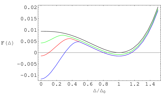
Figure 3: Free energy for $\alpha=\beta=1$ as a function of chemical potential $\mu$ (in units of $\Delta_{0}$): $0$ (black), $0.4$ (green), $0.6$ (red), and $0.8$ (blue).

The analysis of the above formulas and the corresponding plot of Fig.3 reveals a local maximum that resides at $\Delta_{0}e^{-14/3}$ for $\mu=0$ and gradually moves rightward as $\mu$ increases. In contrast, the global minimum located at $\Delta_{0}$ first comes down slightly and then rises with increasing $\mu$ but, otherwise, retains its position up to $\mu_{c}\approx 0.6\Delta_{0}$.

Upon approaching $\mu_{c}$ the free energy computed with the use of the approximate solution (18) shows a behavior suggestive of a first order transition. This observation should be contrasted with the conjecture that for $\mu=0$ the corresponding transition is of infinite order.appelquist

The above value of $\mu_{c}$ differs from that obtained in Ref. 4, in which a first order transition was found at $\mu_{c}^{\prime}\approx 1.2\Delta_{0}$. It should be noted, however, that in their calculation of the free energy, the authors of Ref. 4 introduced the chemical potential as the lower limit in the integration over $\xi_{p}$ rather than $E_{p}$, which assignment becomes inaccurate for $\mu\sim\Delta_{0}$.

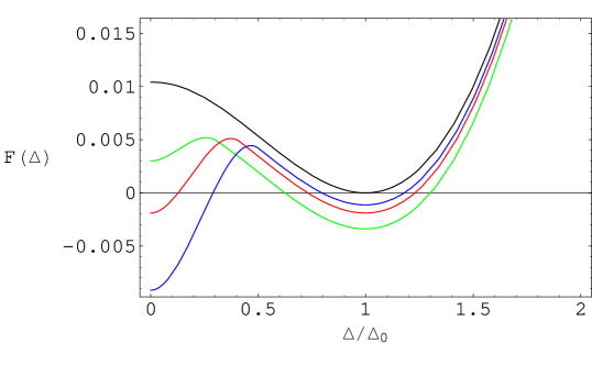
Figure 4: Free energy for $\alpha=1/2$, $\beta=1$ as a function of chemical potential $\mu$ (in units of $\Delta_{0}$): $0$ (black), $0.5$ (green), $0.7$ (red), and $0.8$ (blue).

Lastly, in Fig.4 we present the free energy for $\alpha=1/2$ and $\beta=1$, which choice of the parameter values corresponds to the physically relevant problem of the Coulomb interacting electrons in an infinite stack of graphene layers semenoff ; dvk . The behavior exhibited by Fig.4 is still indicative of a first order transition at $\mu_{c}\approx 0.7\Delta_{0}$.

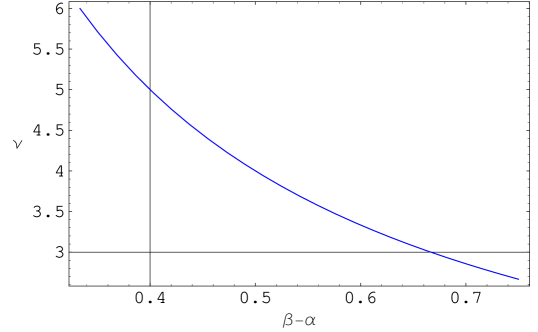
Figure 5: Exponent $\nu$ in the maximum gap $\Delta_{0}\propto({\tilde{g}}-{\tilde{g}}_{c})^{\nu}$ as a function of $\beta-\alpha$.

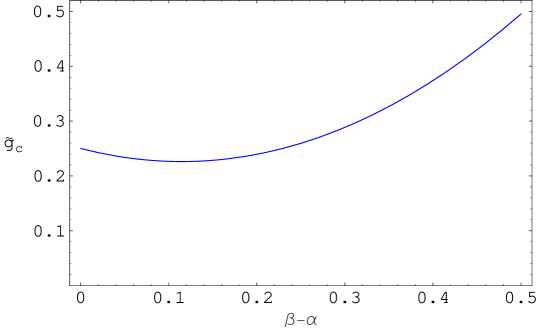
Figure 6: Critical coupling ${\tilde{g}}_{c}$ as a function of $\beta-\alpha$.

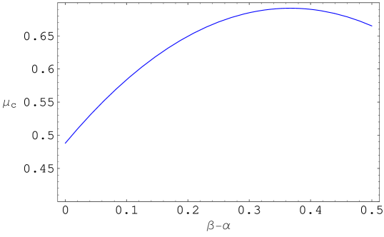
Figure 7: Critical value of the chemical potential $\mu_{c}$ (in units of $\Delta_{0}$) as a function of $\beta-\alpha$.

In fact, a more extensive analysis shows that the above pattern appears to be common in the entire range of parameters $\beta/3\leq\alpha\leq\beta$. The maximum gap $\Delta_{0}$ (Fig.5) and the critical coupling $g_{c}$ (Fig.6), plotted as functions of the difference $\beta-\alpha$ agree well with the analytical results given by Eqns.13 and 14, respectively. The dependence of the critical value of the chemical potential $\mu_{c}$ (Fig.7) upon that parameter turns out to be somewhat less pronounced, though.

Before concluding, we comment on our assumption of a spatially uniform order parameter (that allows one to focus solely on the dependence of $\Delta$ on the relative momentum $\bf p$ of particle-hole pairs). Relaxing this simplifying assumption enables one to extend the class of solutions and search for possible Fulde-Ferrel-Larkin-Ovchinnikov (FFLO) states where the order parameter demonstrates periodic spatial variations. Although we choose to postpone a further analysis of this more general case until future work, our preliminary results suggest that the FFLO-like states may only provide a viable alternative to the uniform ground state close to the critical value of the chemical potential, thus opening the possibility of a sequence (at least, two) transitions that might occur in the vicinity of the aforementioned $\mu_{c}$.

As far as the possible applications of the above results are concerned, we believe that they may prove helpful for resolving a number of outstanding issues pertinent to the physics of the nodal strongly correlated electron systems.

For one, the recent advent of spintronics has brought about an upsurge of interest in the magnetic properties of nonmetallic compounds, including pyrolytic graphite and other degenerate semimetals which can potentially harbor a latent excitonic instability responsible for the emergence of a (possibly weak, yet robust) ferromagnetism, in accordance with the scenario put forward in Ref. 7. Although the other recent suspects for the role of excitonic ferromagnet, hexaborides,rice have been largely disqualified on the basis of the experimentally established extrinsic origin of the observed ferromagnetic response,bennett the reports of a weak ferromagnetism in some graphitic samples graphite has not yet been properly explained.

Whether the magnetism of graphite is associated with a genuine many-body phenomenon such as the bulk Peierls (charge and/or spin) instability in gapless semimetals or it has a more mundane nature related to the presence of (non)magnetic bulk and/or surface defects, there remains a compelling need for a comprehensive analysis of novel, non-BCS-like, pairing scenarios in nonmetallic systems with long-range interactions. In particular, it is important to ascertain the extent to which the customary practice (see Refs. 11 and references therein) of replacing the unscreened Coulomb interaction with the Hubbard-like on-site repulsion (the only motivation for which seems to be a greater suitability of the latter for numerical simulations) would allow one to understand the physics of nonmetallic systems.

Also, the idea of an incipient phase transition reminiscent of the phenomenon of chiral symmetry breaking has recently gained an additional popularity after a number of (formally identical but physically distinct) adaptations of the relativistic QED₃ theory were discussed in such contexts as the antiferromagnet-to-spin liquid and pseudogap-to-charge/spin density wave transitions in underdoped cuprates.qed

Other examples, including a conjectured second pairing transition in $d$-wave superconductors yukawa or $f$-pairing in dichalkogenides,antonio have been discussed in the context of the (pseudo)relativistic 3D Higgs-Yukawa model. Despite the differences in their underlying physics, all of the aforementioned problems appear to be amenable to a unified description in the framework of Eq.(4), with the parameter values chosen as $\alpha_{\text{QED}}=\beta_{\text{QED}}=1$ or $\alpha_{\text{HY}}=0$, $\beta_{\text{HY}}=1$. Yet another formally related pairing problem is that of color superconductivity in QCD₄ where the integral kernel in the analog of Eq.(4) behaves as $U(p-q)\propto\ln|p-q|$.

The solutions similar to Eq.(15) were also obtained in the earlier studies of pairing between incoherent quasiparticle excitations mediated by spin fluctuations in $d$- and $p$-wave superconductors.chubukov1 In that context, the energy (albeit not momentum) dependent gap function was found to satisfy a counterpart of Eq.(4) with $\alpha=\beta=1/2$.

In summary, we carried out the analysis of the excitonic pairing instability in nodal fermion systems, characterized by a power-law DOS and long-range pairwise interaction potentials. We found non-BCS solutions of the corresponding gap equation at various finite values of the chemical potential. We also computed the free energy and studied its dependence on the chemical potential, thus gaining further insight into the nature of the transition in question. We expect these results to be of interest for a broad range of physical problems involving nodal fermions.

In particular, we observed that the systems with shorter-ranged interactions (lower values of $\alpha$) and/or stronger DOS suppression (higher values of $\beta$) tend to manifest a stronger propensity towards excitonic pairing. The excitonic order emerges at sufficiently strong repulsive couplings and survives up to a finite critical doping by excess carriers. The observed differencies in the behavior at zero and finite $\alpha$ should serve as a warning against replacing genuinely long-ranged (e.g., Coulomb) interactions with short-ranged ones, largely for the sake of a greater ease of the calculations.

This research was supported by NSF under Grant DMR-0349881 and, in part, by ARO under Contract DAAD19-02-1-0049. One of the authors (DVK) acknowledges valuable communications with A. Chubukov, Y. Kopelevich, and V. Gusynin as well as the hospitality at the Aspen Center for Physics where some of this work was carried out.

References

- (1) G. Semenoff, Phys. Rev. Lett.53, 2449 (1984); F. D. M. Haldane, ibid 61, 2015 (1988); J. Gonzalez, F. Guinea, and M. A. H. Vozmediano, Phys. Rev. Lett. 69, 172 (1992); ibid 77, 3589 (1996); Nucl. Phys. 406, 771 (1993); ibid B424, 595 (1994); Phys. Rev. B59, 2474 (1999); ibid B63, 134421 (2001).
- (2) A. H. Castro-Neto, Phys. Rev. Lett. 86, 8342 (2001); B.Uchoa, A. H. Castro-Neto, and G.G.Cabrera, Phys. Rev. B69, 144512 (2004); cond-mat/0409471.
- (3) D. V. Khveshchenko, Phys. Rev. Lett. 87, 246802 (2001); ibid 87, 206401 (2001); D. V. Khveshchenko and H. Leal, Nucl. Phys. B687, 323 (2004).
- (4) E. V. Gorbar, V. P. Gusynin, V. A. Miransky, and I. A. Shovkovy, Phys. Rev.B66, 045108 (2002); Phys. Lett. A313, 472 (2003).
- (5) T. Appelquist, D. Nash, and L. Wijewardhana, Phys. Rev. Lett.60, 2575 (1988); T. Appelquist, J. Terning, and L. Wijewardhana, ibid 75, 2081 (1995); T. Appelquist, A. G. Cohen, and M. Schmaltz, Phys. Rev. D60, 045003 (1999).
- (6) R. Haslinger and A. V. Chubukov, Phys. Rev. B67, 140504 (2003); ibid B68, 214508 (2003); E. Tsoncheva and A.V. Chubukov, cond-mat/0503512.
- (7) B.A Volkov, Yu. V. Kopaev and A.I. Rusinov, Sov. Phys. JETP 41, 952 (1975); B.A Volkov, A.I. Rusinov, and R.K. Timerov, ibid 43, 589 (1976).
- (8) M. E. Zhitomirsky, T. M. Rice, and V. I. Anisimov, Nature 402, 251 (1999); V. Barzykin and L. P. Gorkov, Phys. Rev. Lett. 84, 2207 (2000); L. Balents and C. M. Varma, ibid 84, 1264 (2000); E. Bascones, A. A. Burkov, and A. H. MacDonald, ibid 89, 086401 (2002); L. Balents, Phys. Rev.B62, 2346 (2000); M. Y. Veillette and L. Balents, ibid B65, 014428 (2002).
- (9) M. C. Bennett et al, Phys. Rev. B69, 132407 (2004).
- (10) Y. Kopelevich et al, J. Low Temp. Phys.119, 691 (2000); P. Esquinazi et al, Phys. Rev. B66, 024429 (2002).
- (11) A. L. Tchougreeff and R. Hoffmann, J. Phys. Chem.96, 8993 (1992); F. R. Wagner and M. B. Lepetit, ibid 100, 11050 (1996); G.Baskaran and S.A.Jafari, Phys. Rev. Lett.89, 016402 (2002); K. Kusakabe and M. Maruyama, Phys. Rev. B67, 092406 (2003); N.M.R.Perez, M.A.N.Araujo, and D.Bozi, ibid B70, 195122 (2004); N.M.R.Perez and M.A.N.Araujo, cond-mat/0502249.
- (12) D. H. Kim and P. A. Lee, Annals of Physics, 272, 130 (1999); I. F. Herbut, Phys. Rev. Lett. 88, 047006 (2002); Phys. Rev. B66, 094504 (2002); Z. Tesanovic, O. Vafek, and M. Franz, Phys. Rev. B65 (2002) 180511; M. Franz, D. E. Sheehy, and Z. Tesanovic, Phys. Rev. Lett. 88, 257005 (2002).
- (13) M. Vojta, Y. Zhang, and S. Sachdev, Phys. Rev. Lett. 85, 4940 (2000); Phys. Rev. B62, 6721 (2000); D. V. Khveshchenko and J. Paaske, Phys. Rev. Lett. 86, 4672 (2001).
- (14) A. Abanov, A. V. Chubukov, and A. M. Finkelstein, Europhys. Lett. 54, 488 (2001); A. Abanov, A. V. Chubukov, and J. Schmalian, ibid 55, 369 (2001); A. V. Chubukov and J. Schmalian, cond-mat/0507562.