From exotic phases to microscopic Hamiltonians

Abstract

We report recent analytical progress in the quest for spin models realising exotic phases. We focus on the question of ‘reverse-engineering’ a local, SU(2) invariant S=1/2 Hamiltonian to exhibit phases predicted on the basis of effective models, such as large-$N$ or quantum dimer models. This aim is to provide a point-of-principle demonstration of the possibility of constructing such microscopic lattice Hamiltonians, as well as to complement and guide numerical (and experimental) approaches to the same question. In particular, we demonstrate how to utilise peturbed Klein Hamiltonians to generate effective quantum dimer models. These models use local multi-spin interactions and, to obtain a controlled theory, a decoration procedure involving the insertion of Majumdar-Ghosh chainlets on the bonds of the lattice. The phases we thus realise include deconfined resonating valence bond liquids, a devil’s staircase of interleaved phases which exhibits Cantor deconfinement, as well as a three-dimensional $U(1)$ liquid phase exhibiting photonic excitations.

1 Introduction

In the early 1970s, Anderson and Fazekas andersonfazekas proposed that the $S=1/2$ quantum Heisenberg antiferromagnet on the triangular lattice should exhibit a new type of phase, the resonating valence bond (RVB) liquid. Unlike a conventional Néel phase, the RVB liquid would retain the full symmetry of the spin Hamiltonian, and thus neither break spatial nor time-reversal symmetries. In addition, an odd number of sites per unit cell in such a state also implies the existence of an unambiguous Mott insulator not adiabatically connected to a simple band insulator.

Alas, this was not to be: the triangular $S=1/2$ antiferromagnet exhibits Néel order. While a simple collinear two-sublattice Néel structure is precluded by the non-bipartiteness of the triangular lattice, the spin order distinguishes three sublattices, on which the directions of the spin order parameter are oriented at 120^omisguich-lhuillier .

The question whether an RVB liquid could exist, as a matter of principle, was left unanswered. Interest in this problem was greatly intensified with the advent of high-temperature superconductivity and the proposal that the superconducting phase effectively derived from doping a parent RVB liquid AndersonScience .

In the following, the RVB liquid continued to be elusive. One obstacle was that, when destabilising a bipartite Néel state, e.g. by adding frustrating interactions, the competing ground state would typically tend to break some other local symmetry. A particular prominent example is the valence bond solid, in which the order parameter leaves the SU(2) invariance intact (as it involves bond amplitudes $\langle{\bf S}_{i}\cdot{\bf S}_{j}\rangle$ rather than a single spin, $\langle{\bf S}\rangle$), but nonetheless breaks translational symmetry.

While no RVB liquid had thus become available, a proof of its non-existence was not forthcoming either, and the search thus continued. One route being followed was to study an increasing number of Hamiltonians numerically in the hope of isolating the most promising candidates misguich-lhuillier . A second one was to investigate analytically tractable models – at the expense of quantum chemical realisability – and attempt a direct demonstration of the existence of the RVB liquid. One possibility, for instance, consists of enlarging the symmetry group to obtain a large-$N$ theory rslargeN , although the applicability to the small-$N$ regime remains unsettled.

In this presentation, we review how the second strategy can be carried through entirely: we describe how, in a local SU(2) invariant $S=1/2$ Hamiltonian, one can demonstrate the existence of an RVB liquid. As a byproduct, we can in fact show that a range of other interesting valence bond dominated phases can similarly be shown to exist.

The two conceptually separate steps in this demonstration are (i) how to transform the SU(2) Hilbert space into one of valence bonds by using a local Hamiltonian and (ii) how to construct an effective Hamiltonian in the reduced valence bond (‘dimer’) space that can be demonstrated to lead to a liquid phase.

Step (ii) has as its starting point the seminal work by Rokshar and Kivelson (RK) Rokhsar88 , who formulated their quantum dimer model (QDM) in the hope of its exhibiting a liquid phase. Whereas that hope was not fulfilled, it was later shown MStrirvb that the RK-QDM on the triangular lattice indeed does exhibit such a liquid phase. A central ingredient in this demonstration was the fact that at a particular point in parameter space (the RK point), the RK-QDM is exactly soluble. It was thus possible to demonstrate that all local correlators formulated in terms of dimers are short-ranged. This was combined with numerical evidence for the continuity of the physics at this point into an extended phase (see in particular the recent work by the Lausanne group lausanneGFMC , also covered in this workshop).

The solution of step (i) builds on a thread of work initiated by Klein Klein , who wrote down a class of model Hamiltonians which have nearest-neighbour valence bond coverings as their ground states. This work was carried further by Chayes, Chayes and Kivelson chayeschayeskivelson , but, in the absence of the dimer liquid, activity in this direction waned.

In the following, we first concentrate on step (i). We start with with a qualitative account of Klein models Klein , and how they lead to valence bond ground states. In particular, we argue that supplementary ground states can be excluded using a decoration procedure, so that we are left with a low-energy sector of degenerate nearest neighbour valence bond ground states, which we refer to as dimer coverings. An example of such a covering is given in Fig. 1.

We then turn to the construction of effective quantum dimer Hamiltonians within this subspace using the RK overlap expansion. We construct operators which mimick the potential and kinetic terms of the RK-QDM. We argue that the decoration procedure introduced above can also be used to control the size of unwanted additional terms. Readers interested in a detailed account of the technicalities are referred to our original publication, Ref. rmsklein

This is followed by a brief account of the new phases attained by this construction. These include the abovementioned SU(2) invariant RVB liquid phase.

In closing the introduction, we would like to draw the reader’s attention to a complementary piece of work by Fujimoto fujimotoklein , who constructs Hamiltonians realising the RK-QDM for valence bond wavefunctions.

2 Spin Hamiltonians as projectors

The Heisenberg Hamiltonian

$$H_{Heis}=J\sum_{\langle i,j\rangle}\vec{s}_{i}\cdot\vec{s}_{j}$$ (1)

can be considered to be a projector:

$$H_{Heis}=\sum_{\langle i,j\rangle}\hat{P}_{\{ij\}}^{S=1}$$

which exacts an energy $J$ if the pair of spins $\{i,j\}$ has total spin $S=1$; a singlet $S=0$ costs no energy.

The projectors $\hat{P}$ on different bonds do not commute, as one would expect for a quantum model. Writing down a ground state for the full Hamiltonian does therefore, in general, not reduce to minimising the Hamiltonian for each bond separately. This is of course ultimately what makes it so much more difficult to write down an exact ground state for a quantum rather than a classical spin model.

The big insight of Klein was that there exists a half-way house. For different operators to be simultaneously minimisable does not in fact require that they commute. Rather, by a judicious choice of the properties of the projectors, it can become possible to find a subspace of the Hilbert space which is annihilated by all the projectors, even though they do not commute.

To achieve this, Klein proposed defining the projectors not for each single bonds, as is the case for the usual Heisenberg model, but instead for the neighbourhood $\mathcal{N}(i)$ of each site $i$. This neighbourhood consists of a site and its $z-1$ nearest neighbours. Again, the projector is constructed so that its exacts an energy cost $J$ only when the spins in $\mathcal{N}(i)$ are in the maximally allowed spin state, $S=z/2$.

One can thus write the Klein Hamiltonian as

$$H_{K}=\sum_{i\in\Lambda}\hat{P}^{S=z/2}_{\mathcal{N}(i)}\ ,$$ (2)

with $S$ given as

$$\vec{S}_{\mathcal{N}(i)}=\sum_{j\in\mathcal{N}(i)}\vec{s}_{j}$$ (3)

This Hamiltonian corresponds not to a pair interaction as in the Heisenberg case, but rather to a multispin interaction. The larger the neighbourhood ${\mathcal{N}(i)}$, the more spins are involved in this interaction. However, it always remains local.

For instance, for even $z$, one obtains

$$\hat{P}_{\mathcal{N}(i)}=k_{i}\prod_{L=0}^{z_{i}/2-1}\Bigl{[}S_{\mathcal{N}(i)}^{2}-L(L+1)\Bigr{]}\ .$$ (4)

It is now easy to see why this Hamiltonian is minimised by nearest-neighbour valence bond coverings. Such coverings are defined by complete pairings of the sites of the lattice such that each site is paired to form a spin singlet with one of its nearest-neighbours. This implies that the $z$ spins in ${\mathcal{N}(i)}$ can at most sum up to a total spin $S=(z-2)/2$, and hence the corresponding projector $\hat{P}_{\mathcal{N}(i)}$ is guaranteed to annihilate this state.

The simplest representative of this class of Hamiltonians is the Majumdar-Ghosh model majghosh , the one-dimensional chain in which spins interact in neighbourhoods containing three spins, which gives it the alternative appearance of a model with nearest and next-neaerest neighbour interactions.

However, writing down such projectors in itself is of course not the full story. After all, an even simpler Hamiltonian, $H\equiv 0$, would have had all valence bond coverings as ground states as well. If one wants to obtain a quantum dimer model via the Klein route, it is necessary to demonstrate that in fact there are no other ground states for this Hamiltonian.

In some cases, such a demonstration is possible, as for the case of the honeycomb lattice chayeschayeskivelson . In others, it is possible to show explicitly that there are other ground states, as is the case for the square or triangular lattices (see Fig. 2). For the Majumdar-Ghosh chain, Shastry and Sutherland presented a calculation showing that excitations above the dimerised ground states do remain gapped ShasSutherMG .

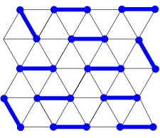
Figure 1: A nearest-neighbour valence bond (dimer) covering for a triangular lattice.

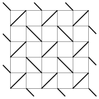
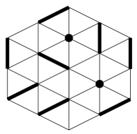
Figure 2: Ground states of the Klein model which are not nearest neighbour valence bond (dimer) coverings of the underlying lattice. These are removed by the decoration procedure.

3 Decoration

This problem of the supernumerary ground states can be taken care of by a decoration procedure (see Fig. 3). Details of the necessary calculations are given in Ref. rmsklein .

Basically, the decoration procedure places an even number, $N$, of supplementary sites between each pair of sites of the original lattice. The parity of the sites per unit cell is left unchanged by this decoration procedure for a lattice of even coordination. In the case of a lattice with odd coordination, one needs to choose $N$ to be a multiple of 4 for this to be the case.

The Hamiltonian for the extended lattice is its Klein Hamiltonian, with the possibility of varying the prefactor for the projectors of a neighbourhood depending whether it contains a site of the original lattice.

\psfrag{a1}{{a1}}\includegraphics[height=126.47249pt]{hex2}

Figure 3: Decoration procedure to remove unwanted ground states, and to obtain a control parameter for the RK overlap expansion.

For the supplementary sites, the projectors are of course of the Majumdar-Ghosh type. Thus, thinking of the supplementary sites on a given bond as a Majumdar-Ghosh chainlet (of finite length $N$), it is clear that its interior will not harbour gapless excitation.

Problems can arise close to the original sites, where several of these chainlets meet, thus enabling any excitations to gain additional kinetic energy as the local coordination is higher there. Repeating the Shastry-Sutherland calculation on the Majumdar-Ghosh model for the present case, we find that it is possible to choose the interaction parameters such that the gap is not destroyed. This calculation is carried out explicitly for the case of the honeycomb lattice in Ref. rmsklein .

Finally, one needs to note that the dimerisations of the decorated lattice can be mapped bijectively onto those of the unprojected one. This follows from the fact that there are only two possible dimerisation patterns for the Majumdar-Ghosh chainlets. As we have chosen $N$ to be even, one of these is compatible with dimers from the original sites both pointing inwards into the chain, and the other with no dimers pointing inwards. These correspond to the presence and absence, respectively, of a dimer on the bond linking the two original sites in the undecorated lattice.

4 Perturbation theory in the dimer manifold

We now turn to the second step in the program – how to get from a valence bond Hilbert space to the desired dimer phases. In essence, we are looking for terms in the Hamiltonian, subleading to the Klein terms, which mimick the RK-QDM when projected onto the valence bond ground state subspace.

The RK-QDM, in pictorial form for the square lattice (for which it was written down originally Rokhsar88 ), has the following form:

$$\scalebox{0.5}{\includegraphics{hqdm.eps}}\ .$$ (5)

It contains two terms, a kinetic and a potential one. Firstly, the resonance term flips a pair of dimers around a plaquette; it has a matrix element $-t$, where $t$ needs to be positive for the quantum dimer model to be analytically tractable in a simple manner. This can often, but by no means always, be arranged.

This term accounts for the resonance move to which the resonating valence bond physics owes its name. The other is a potential term, which exacts an energy cost $v$ for each plaquette that can resonate. In practice, it important as (i) the RK point $v/t$ is often soluble (or straightforwardly simulateable) and (ii) because it can be used to counterbalance ordering tendencies, thus enhancing the disordering effect of quantum fluctuations.

To give meaning to such a pictorial Hamiltonian, we first need to specify precisely what we mean by the pictures of dimers, as the dimer coverings are not orthogonal. Indeed, if we define coverings, $i$, of the lattice with nearest-neighbour valence bonds, we can define an overlap matrix $S$, with matrix elements

$$S_{ij}=\langle i|j\rangle\ ,$$ (6)

allowing us to define an orthonormal basis using the states $\alpha$ as follows:

$$|\alpha\rangle=\sum_{i}(S^{-1/2})_{\alpha,i}|i\rangle\ .$$ (7)

The crucial observation is that, for our decorated lattice, the overlap between two distinct dimer coverings is exponentially small in $N$, the number of sites on the decorating Majumdar-Ghosh chainlets. This follows from the observation that the overlap between two coverings differing in a loop of $n$ dimers is $(1/2)^{n-1}$, and the presence of the chainlets ensures that $n\propto N$.

We can thus identify a basis vector $\alpha$ with its leading principal valence bond covering $i$, the admixture of other coverings $j\neq i$ being exponentially suppressed. In the orthonormalised basis, the matrix elements of the Hamiltonian read

$$H_{\alpha\beta} = (S^{-1/2}\delta HS^{-1/2})_{\alpha\beta}$$ (8)

$$= \sum_{ij}(S^{-1/2})_{\alpha i}\langle i|\delta H|j\rangle(S^{-1/2})_{j\beta}\ .$$ (9)

The calculation of each of the matrices appearing in this expression involves the non-orthogonal dimer coverings, $i$, and can thus be carried out relatively straightforwardly.

For example, in the case of the honeycomb lattice, we use the following perturbing Hamiltonian:

$$\delta H = J\sum_{\langle ij\rangle}\vec{s}_{i}\cdot\vec{s}_{j}+$$ (10)

$$v\sum_{\hexagon}\Bigl{(}(\vec{s}_{1}\cdot\vec{s}_{b_{1}})(\vec{s}_{3}\cdot\vec{s}_{b_{3}})(\vec{s}_{5}\cdot\vec{s}_{b_{5}})$$

$$+(\vec{s}_{1}\cdot\vec{s}_{a_{1}})(\vec{s}_{3}\cdot\vec{s}_{a_{3}})(\vec{s}_{5}\cdot\vec{s}_{a_{5}})\Bigr{)}\ ,$$

where the labeling of the sites is given in Fig. 3. The understanding is that the energy scales $v,J$ occuring here are much smaller than those of the Klein model, so that it suffices to do degenerate perturbation theory.

Plugging the perturbing Hamiltonian (10) into the overlap expansion (9) yields the following quantum dimer Hamiltonian:

$$H_{\alpha\beta} = -Jx^{6(N+1)}\hexagon_{\alpha\beta}+vn_{fl,\alpha}\delta_{\alpha\beta}$$ (11)

$$+ O(vx^{6(N+1)}+Jx^{10(N+1)})$$

$$= -t\hexagon_{\alpha\beta}+vn_{fl,\alpha}\delta_{\alpha\beta}+O(vx^{6(N+1)}+tx^{4N})\ .$$

Here, $n_{fl}$ counts the number of plaquettes which can resonate in a dimer configuration, and $\hexagon_{\alpha\beta}$ denotes a matrix whose elements are non-zero if the the two dimer coverings differ only by a single resonance move, and $x=1/\sqrt{2}$. These thus realise the desired potential and kinetic terms, respectively.

As advertised before, the small parameter of our overlap expansion is effectively $x^{N}$, which can be made arbitrarily small. We need to point out that the interaction responsible for the potential term is of range $N$ in units of nearest-neighbour distances of the decorated lattice. Hence, for $N\rightarrow\infty$, our interaction would cease to be local. However, the expectation is that the actual value of $N$ required for this scheme to work will not be all that large.

The benefit of the decoration scheme is therefore that it provides us with a small control parameter which, unlike in the case of large-$N$ theories, is not related to an enlarged internal symmetry of spin space: we are still dealing with the native SU(2) symmetry.

5 Resulting valence bond phases

Having established how to obtain a RK-QDM from an SU(2) invariant Hamiltonian, we sketch in the following the type of phases which we can realise in this way. The basic difference to bear in mind when comparing to the work on pure RK-QDMs is that here we have additional terms in the Hamiltonian, albeit of small size (controlled by the decoration). Nonetheless, properties which require the fine-tuning of some parameters, such as the existence of multicritical points, will be sensitive to their presence, whereas a stable phase will generically be robust.

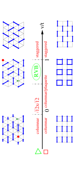
Figure 4: Schematic phase diagram of the RK-QDM on the square and triangular lattices. The cartoons for the triangular lattice depict the presence of fractionalisation and deconfinement for the case of the RVB liquid phase, and its absence for the valence bond solid phases. The RK-QDM model on the square lattice only has solid phases.

5.1 SU(2) invariant RVB liquids

In Fig. 4, we show the phase diagram of the RK-QDM on the triangular lattice. Its most salient feature is the presence of an extended RVB liquid phase including the RK point and the vicinity to its left. As this is a gapped phase, it will be stable to the perturbations included in the Klein-derived quantum dimer Hamiltonian. Our construction thus provides the point-of-principle demonstration that SU(2) invariant RVB liquids do exist.

5.1.1 Fractionalisation

This RVB liquid corresponds to the deconfined phase of an effective Ising gauge theory msf . This is indicated in Fig. 4 in cartoon form. In the columnar phase, separating two monomers creates a domain wall, the tension of which leads to a diverging confining potential between the monomers as their separation is increased.

By contrast, in the liquid phase, a monomer is oblivious to the distance to its partner once their separation exceeds several correlation lengths. The pair can thus be separated at a finite cost in energy – it is deconfined.

This phenomenon is also known as spin-charge separation AndersonScience . This name is due to the observation that removing one electron leaves behind the partner with which it formed a singlet bond (see Fig. 5). One is thus left with a spinless charged hole and an uncharged spin. Separating these two at finite cost in energy thus allows the independent existence of a spin-0 charge-e object and a spin-1/2 charge-0 object. The phenomenon of spin-charge separation is a particular instance of quantum number fractionalisation.

Figure 5: Removing an electron leaves behind a charged hole and an unpaired spin.

5.2 Cantor deconfinement

The phase diagram for the square lattice RK-QDM is not the full story as far as the quantum dimer model derived via the overlap expansion is concerned. This is due to the small correction terms present in Eq. 11. Although exponentially small, they become important close to the phase transition between plaquette and staggered valence bond solid. This happens because the RK Hamiltonian leads to a fix-point action for this phase transition which has a symmetry which is higher than that dictated by the underlying symmetries of the lattice.

In other words, the phase transition in the RK-QDM corresponds to a fine-tuned multicritical point, which fine tuning is undone by the correction terms cantor . We note in passing that this multicritical point is very interesting in its own right. It is an example of a critical point exhibiting deconfinement, whereas the phases it separates are both confined MStrirvb . The phenomenon of such ‘deconfined quantum criticality’ in a more general setting has received a great deal of attention recently dqcp . For an interesting example of a deconfined critical point in a microscopic model, see Ref. alexeidqcp .

\psfrag{C}{\small{columnar}}\psfrag{P}{\small{plaquette}}\psfrag{I}{\small{(in)commensurate}}\psfrag{T}{\small{tilt}}\psfrag{m}{\small{max}}\psfrag{R}{\small{RK point}}\psfrag{0}{\small$0$}\psfrag{inf}{\small$-\infty$}\psfrag{1}{\small$1$}\psfrag{pinf}{\small$\infty$}\psfrag{s}{\small{staggered}}\psfrag{v}{\small$v/t$}\includegraphics[width=411.93767pt]{PHASED-new.eps}

Figure 6: The phase diagram of the generalised RK-QDM on the square lattice. A detailed analysis is given in Ref. cantor . The vertical axis, ’tilt’, is zero in the columnar and plaquette phases, and maximal (i.e. limited by lattice effects) in the staggered phase. Its jump in the RK model, where the RK point is fine-tuned multicritical, is replaced by an ascending devil’s staircase in the Klein-derived quantum dimer model.

The phase diagram resulting instead is shown in Fig. 6. There, the abrupt change from plaquette to staggered valence bond solid is replaced by a continuous growth of an appropriately defined order parameter, the ‘tilt’ cantor . Due to an interplay between a locking potential due to the underlying lattice and the tilt favoured in its absence (which tilt may be incommensurate), the growth is not smooth, but occurs in the form of a devil’s staircase. Provided that no first-order phase transition intervenes, the region close to the RK point is effectively deconfined, a phenomenon we have termed Cantor deconfinement – for the small print, see Ref. cantor .

5.3 Artificial electromagnetism

The long-wavelength description of the QDM on the square lattice is that of a U(1) gauge theory in $d=2+1$. The presence of confinement everywhere, well known from high energy physics, is a consequence of this structure. This makes the existence of the Cantor deconfined region somewhat remarkable. However, in essence this is possible because it occurs in a sector of the gauge theory not covered by the conventional wisdom.

In three dimensions, things are considerably simpler as the existence of a deconfined phase in the corresponding U(1) gauge theory in $d=3+1$ is not precluded on general grounds. In fact, the three-dimensional dimer model, obtained along the lines discussed above, is expected to exhibit a Coulomb phase in which quasiparticles fractionalise. Perhaps just as strikingly, this phase supports transverse collective excitations which are completely analogous to photons in conventional electromagnetism but which represent an emergent excitation: they represent a collective excitation of the SU(2) spins-1/2 on the simple cubic lattice. Endowed with the Klein Hamiltonian, this system can act as ether for an artificial electromagnetism artificiallight .

References

- (1) P. Fazekas and P. W. Anderson, Philos. Mag. 30, 23 (1974).
- (2) For a review of numerical work, see G. Misguich and C. Lhuillier, cond-mat/0310405.
- (3) P. W. Anderson, Science 235, 1196 (1987).
- (4) N. Read and S. Sachdev, Phys. Rev. Lett. 66, 1773 (1991).
- (5) D. S. Rokhsar and S. A. Kivelson, Phys. Rev. Lett. 61, 2376 (1988).
- (6) R. Moessner and S. L. Sondhi, Phys. Rev. Lett. 86, 1881 (2001).
- (7) A. Ralko, M. Ferrero, F. Becca, D. Ivanov and F. Mila, Phys. Rev. B 71, 224109 (2005).
- (8) D. J. Klein, J. Phys. A. Math. Gen. 15, 661 (1982).
- (9) J. T. Chayes, L. Chayes, and S. A. Kivelson, Commun. Math. Phys. 123, 53 (1989).
- (10) K. S. Raman, R. Moessner and S. L. Sondhi, Phys. Rev. B 72, 064413 (2005).
- (11) S. Fujimoto, Phys. Rev. B 72, 024429 (2005).
- (12) C. K. Majumdar and D. K. Ghosh J. Math. Phys. 10, 1388 (1969).
- (13) B. S. Shastry and B. Sutherland, Phys. Rev. Lett. 47, 964 (1981).
- (14) R. Moessner, S.L. Sondhi and Eduardo Fradkin, Phys. Rev. B 65, 024504 (2002).
- (15) E. Fradkin, D. A. Huse, R. Moessner, V. Oganesyan, and S. L. Sondhi, Phys. Rev. B 69, 224415 (2004); A. Vishwanath, L. Balents, and T. Senthil, Phys. Rev. B 69, 224416 (2004).
- (16) T. Senthil, Ashvin Vishwanath, Leon Balents, Subir Sachdev and M. P. A. Fisher, Science 303, 1490 (2004).
- (17) A. M. Tsvelik, Phys. Rev. B 70, 134412 (2004) and references therein.
- (18) R. Moessner and S. L. Sondhi, Phys. Rev. B 68, 184512 (2003); M. Hermele, M. P. A. Fisher and L. Balents, Phys. Rev. B 69, 064404 (2004).